Abstract
Extreme precipitation events severely impact agriculture, reducing yields and land use efficiency. The spatiotemporal distribution of Total Column Water Vapor (TCWV), the primary gaseous form of water, directly influences sustainable agricultural management. This study, through multi-source data fusion, employs methods including the Mann–Kendall test, sliding change-point detection, wavelet transform, pixel-scale trend estimation, and linear regression to analyze the spatiotemporal dynamics of global TCWV from 1959 to 2023 and its impacts on agricultural systems, surpassing the limitations of single-method approaches. Results reveal a global TCWV increase of 0.0168 kg/m2/year from 1959–2023, with a pivotal shift in 2002 amplifying changes, notably in tropical regions (e.g., Amazon, Congo Basins, Southeast Asia) where cumulative increases exceeded 2 kg/m2 since 2000, while mid-to-high latitudes remained stable and polar regions showed minimal content. These dynamics escalate weather risks, impacting sustainable agricultural management with irrigation and crop adaptation. To enhance prediction accuracy, we propose a novel hybrid model combining wavelet transform with LSTM, TCN, and GRU deep learning models, substantially improving multidimensional feature extraction and nonstationary trend capture. Comparative analysis shows that WT-TCN performs the best (MAE = 0.170, R2 = 0.953), demonstrating its potential for addressing climate change uncertainties. These findings provide valuable applications for precision agriculture, sustainable water resource management, and disaster early warning.
1. Introduction
In 2024, severe typhoons in regions such as China and the United States triggered extreme precipitation events, severely affecting agricultural land systems. These events resulted in reduced crop yields and decreased land use efficiency [1,2]. Such precipitation events are closely linked to anomalous increases in Total Column Water Vapor (TCWV), which, as the primary form of water vapor, directly impacts the sustainability of agricultural land management by regulating precipitation, soil moisture, and climatic conditions [3,4]. Abnormal fluctuations in water vapor content can modify irrigation water requirements or influence the ecological functions of the land surface through evapotranspiration, thereby posing risks to food security and ecosystem stability [5,6,7,8]. In the context of intensifying climate change, the growing frequency of extreme weather events further highlights the pivotal role of water vapor forecasting in optimizing land use decisions [9,10,11]. Therefore, systematically analyzing the laws governing the spatiotemporal variation of TCWV and developing high-precision predictive models are not only scientific necessities for mitigating climate risks but also critical foundations for improving the effectiveness of agricultural land management and ensuring the sustainable use of land resources.
Numerous researchers in the fields of land and environmental science have conducted extensive studies on TCWV across different regions to elucidate its role in agricultural land system management. Johnson et al., based on data from the Amazon Basin, found that increased TCWV is associated with enhanced rainfall intensity, affecting irrigation and planting decisions for crops such as rice and coffee [4]. You et al., through analysis of 2022 Pakistan rainfall data, showed that elevated TCWV is related to flood events, impacting the production and land management of crops like wheat and rice [12]. These findings indicate that TCWV variations directly affect tropical agricultural management. Borger et al., based on data from the southeastern United States, found that increased TCWV alters precipitation patterns, influencing irrigation needs and land use efficiency for corn and soybeans [13]. Kim et al., based on data from the Sahel region of Africa, indicated that TCWV variations lead to irregular rainfall, increasing management challenges for millet and sorghum cultivation [14]. In other global regions, similar water vapor variation patterns also affect agricultural management. In China, Ayantobo et al., based on data from 1980 to 2016, found that the gradient of decreasing water vapor content from east to west corresponds to regional variations in agricultural irrigation demands [15]. Ren et al., through analysis of precipitable water data in China from 1958 to 2020, confirmed that the rising trend in water vapor is associated with increased flood events, posing challenges to agricultural land stability [16]. These analyses underscore the profound impact of TCWV variability on the functions of agricultural land at regional scales, elucidate the dynamic relationships between TCWV and the functionality of agricultural land systems across different regions, and provide a scientific basis for further predicting the effects of water vapor changes on agricultural production.
To address the impacts of water vapor changes on agricultural land systems, researchers have conducted extensive predictive studies to support science-based decision-making in land management. Early studies primarily relied on traditional methods, such as regression models [17] and conditional probability models [18], laying a preliminary foundation for water vapor forecasting. These approaches performed reliably under simple linear conditions but exhibited limitations in complex climate scenarios. In recent years, data-driven models and machine learning algorithms have markedly enhanced predictive capabilities [19,20]. Chen et al. utilized Support Vector Machines (SVM) to analyze water vapor time series, improving the accuracy of short-term forecasts [21], thereby providing an initial demonstration of machine learning applications in nonlinear modeling. With further technological advancements, neural network models have gained wider application in water vapor forecasting, pushing the field forward. Shi et al. applied a convolutional neural network (CNN) to predict TCWV in China, effectively enhancing the extraction of temporal features [22]. Building on this progress, Bai et al. utilized residual networks to improve the stability of long-term forecasts [23]. Similarly, Xiao et al. employed a temporal convolutional network (TCN) to refine the modeling precision of nonlinear meteorological variables [24,25], while Chen et al. harnessed the nonlinear strengths of a Long Short-Term Memory (LSTM) model to bolster the robustness of regional water vapor predictions based on meteorological data [26]. Diouf et al. improved prediction accuracy using the ARIMA model, advancing forecasting technologies [27]. Although some progress has been made in the theory and methods of TCWV prediction, limitations persist in global-scale predictions, particularly in their application to major agricultural regions, given the important role TCWV plays in sustainable agricultural systems. This challenge primarily arises from the inherent complexity of water vapor dynamics on a global scale, where existing models, such as CNN and ARIMA, often struggle to adequately handle multidimensional features and non-stationary trends. Therefore, there is still potential for further improvement in TCWV prediction.
Although previous studies have extensively explored the analysis and forecasting techniques of TCWV at regional scales, systematic investigations of water vapor dynamics at the global scale, particularly in major agricultural regions, remain limited, and existing prediction models require improvements in accuracy and applicability. To address these gaps, this study proposes the following objectives: (1) integrate ERA5 datasets, NOAA global observation sequences, and ground-based data to systematically analyze the spatiotemporal variations of global TCWV from 1959 to 2023 and their impacts on agricultural land systems; (2) combine wavelet transform with various deep learning models to develop a novel hybrid prediction model (WT-LSTM/TCN/GRU), enhancing TCWV forecasting accuracy; and (3) leverage the analysis and prediction results to enhance agricultural water management and optimize land use decisions, thereby promoting sustainable agricultural development.
2. Materials and Methods
2.1. Study Area
The study area encompasses the regional distribution across all seven continents and four oceans, as illustrated in Figure 1. The analysis targets systematically classified climatic zones and geographical features, including tropical regions (e.g., the Congo Basin in Africa, the Amazon Rainforest in South America), monsoon regions (South Asia and Southeast Asia), mid-latitude regions (central North America, western Europe), polar regions (the Arctic Circle and Antarctica), and arid regions (e.g., parts of the Sahara Desert). These categories encompass the world’s major climatic zones, each exhibiting distinct water vapor variation characteristics.
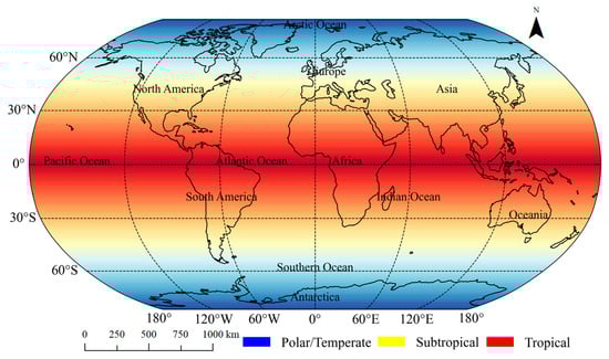
Figure 1.
Overview of the study area, where blue represents polar and temperate regions, yellow indicates subtropical areas, and red denotes tropical zones.
2.2. Data Sources and Processing
This study utilized the fifth-generation atmospheric reanalysis dataset, ERA5, developed by the European Centre for Medium-Range Weather Forecasts (ECMWF) [28,29]. ERA5 integrates global observational data with advanced meteorological models, providing high-accuracy reanalysis data with global coverage. The dataset has a spatial resolution of 0.25° × 0.25° latitude-longitude grid (approximately 27 km × 27 km at the equator) and an hourly temporal resolution. For this study, monthly total column water vapor (TCWV) data, expressed in kilograms per square meter (kg/m2), were extracted for the period 1959 to 2023, representing the total water vapor content from the Earth’s surface to the top of the atmosphere. Thus, the temporal resolution used in our analysis is monthly, which balances computational efficiency with the need to capture seasonal and long-term TCWV trends. ERA5 was selected for its superior spatiotemporal resolution and comprehensive data assimilation, outperforming other reanalysis datasets for capturing global water vapor variability.
To ensure the accuracy and reliability of the data, this study incorporated the Integrated Global Radiosonde Archive (IGRA) dataset from the National Oceanic and Atmospheric Administration (NOAA) as a supplementary validation [30]. IGRA provides vertical profiles of temperature, humidity, and pressure from over 1500 meteorological stations distributed globally. Although its station density is limited, the distribution covers major climate zones, primarily concentrated in the Northern Hemisphere and land areas. Data availability extends from 1905 to near real-time. The validation process involved comparing IGRA data with the nearest ERA5 grid points during the 1959–2023 period, with results showing a correlation coefficient above 0.9 and an average bias less than 1 kg/m2. For example, in the scatter plot for a U.S. site, R2 reached 0.948 and MAE was 0.189 kg/m2 (see Supplementary Figure S1 and Table S1), confirming the consistency and reliability of ERA5 TCWV data. By integrating these independent observations with ERA5 through cross-validation, this study constructed a comprehensive global TCWV dataset spanning 1959–2023, laying a solid foundation for analyzing its spatiotemporal dynamics.
2.3. Methods
This study aims to analyze the spatiotemporal variation characteristics of global TCWV and its impact on agricultural land systems through multi-source data fusion and deep learning models, while improving the prediction accuracy of TCWV changes. The technical workflow of the study is shown in Figure 2. First, Figure 2 (Step 1) presents the data sources used in this study. We integrated the ERA5 reanalysis dataset, NOAA global observational series, and ground station measurement data to build the foundation for global TCWV analysis. The study data covers the period from 1959 to 2023, spanning 65 years, forming a long-term time series, where “long-term time series” is defined as a data span exceeding 60 years. This time range effectively reflects the long-term trends and cyclical fluctuations of climate change.
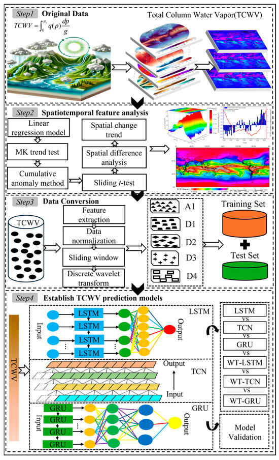
Figure 2.
Technical roadmap for spatial and temporal characterization and prediction of global TCWV. Step 1, Multi-source data integration. Step 2, TCWV spatiotemporal dynamic analysis. Step 3, Wavelet transform data processing. Step, 4 Establishment of TCWV prediction model.
Next, as shown in Figure 2 (Step 2), various methods were applied to comprehensively analyze the spatiotemporal trends of global TCWV. For temporal change analysis, linear regression models and cumulative anomaly sequence analysis were applied. The former is suitable for quantifying the long-term trend of TCWV content, while the latter helps to reveal mutation features and phase changes within the trend. For spatial change analysis, pixel-scale trend estimation methods were used, which effectively capture the global spatial distribution and variation patterns of TCWV, accommodating spatial heterogeneity. The significance of the trends was assessed through statistical tests, specifically including the Mann–Kendall non-parametric test and dynamic sliding t-test. The Mann–Kendall test is robust to non-normal distributions and less sensitive to outliers, making it suitable for verifying the statistical significance of changes in time series. The dynamic sliding t-test adjusts the subsequence length dynamically to improve the precision of detecting mutation points, used to evaluate the significance of spatial distribution changes. Compared to a single method (e.g., ARIMA), the combination of these methods is better suited to address the nonlinearity and spatial complexity of TCWV, comprehensively revealing its spatiotemporal dynamics.
Figure 2 (Step 3) illustrates the data processing workflow. We performed feature extraction and normalization to ensure the consistency and standardization of the input data. Additionally, to enhance data diversity and richness, a sliding window approach was adopted, and discrete wavelet transform was applied for multi-scale decomposition, thereby improving the stability and convergence of the model. This processing step ensured the comprehensive capture of complex spatiotemporal variations.
Finally, Figure 2 (Step 4) describes the development of the prediction model. We propose a hybrid prediction model that combines the multi-scale decomposition capabilities of Discrete Wavelet Transform with the advantages of deep learning time series modeling, constructing three coupled models: WT-LSTM, WT-TCN, and WT-GRU. Specifically, Discrete Wavelet Transform decomposes the TCWV time series into high-frequency (A1) and low-frequency (D1–D4) subsequences, where the high-frequency subsequence captures short-term fluctuations, and the low-frequency subsequences reflect long-term trends. These subsequences are then input into LSTM, TCN, and GRU models for independent training, and the predictions are reconstructed through wavelet inverse transform. Compared to existing studies, this research innovatively applies and compares three deep learning models (LSTM, TCN, GRU) to optimize global-scale TCWV predictions, addressing the nonstationarity and multi-dimensional features of the data. By comparing with single models, the optimal prediction scheme is determined, thereby enhancing model applicability and prediction accuracy. The dataset was divided into a training set (80%) and a validation set (20%), and the model’s prediction performance was comprehensively evaluated by comparing it with actual observed data. Through these methods, this study deepens the understanding of global TCWV spatiotemporal dynamics and significantly improves the prediction accuracy of TCWV.
2.3.1. Linear Fitting and Cumulative Averaging
The long-term time-series variations of TCWV are complex. To thoroughly analyze its interannual change trends, this study employs linear regression analysis [31], establishing a regression model between the annual TCWV sequence and the corresponding years with the expression presented as follows:
In this model, represents the annual mean TCWV content at time point , denotes the intercept term, signifies the regression slope (i.e., the climate tendency rate), which is amplified by a factor of 10 to characterize the strength of the trend, is the time variable, and represents the random error term. This regression model elucidates the long-term evolutionary trend of TCWV. However, when the sequence is influenced by significant random noise or periodic disturbances, a single linear regression approach may fail to adequately capture local dynamics. To address this, this study further introduces the cumulative anomaly sequence analysis method, which enhances the robustness of trend detection by computing and accumulating the anomaly values of the sequence. Its mathematical expression is as follows:
where denotes the cumulative distance level at time point , is the TCWV value in the series, and is the long-term mean of the series. The calculation formula is as follows:
By plotting the cumulative anomaly curve, the long-term evolutionary trends and phased changes in the TCWV time series can be clearly discerned. Linear regression was implemented using MATLAB (version 2020), with the trend rate multiplied by 10 to represent decadal changes. Cumulative anomaly sequence analysis was conducted in MATLAB for computation and visualization to identify phased changes in the TCWV time series. The integrated application of linear fitting and the cumulative anomaly method provides a multidimensional perspective for the dynamic management of water in agricultural land systems.
2.3.2. Mann–Kendall Nonparametric Trend Test and Dynamic Sliding t Analysis
To evaluate the statistical significance of trends in TCWV changes and to investigate their potential climatic abrupt change characteristics, this study integrates the Mann–Kendall nonparametric trend test with dynamic sliding t-statistical analysis to achieve a comprehensive assessment of state transitions in the climate system. Climatic abrupt change refers to a phenomenon in which the climate system undergoes a sudden shift from one stable state to another, typically manifested as significant changes in statistical properties [32]. The Mann–Kendall trend analysis, which does not require assumptions about sample distribution and exhibits low sensitivity to a few outliers, is widely applied in the abrupt change analysis of meteorological time series [33,34]. The calculation formula for its standard normal distribution statistic is as follows:
where is the cumulative sum of ranked difference signs and is the variance of , calculated as follows:
At a given significance level , when , it indicates that the sequence exhibits a significant trend change. By processing the time series in reverse order and plotting the intersection of the and curves within the confidence interval (where is the standardized normal value of the forward cumulative statistic, and is the standardized normal value of the inverse cumulative statistic), the onset time of a climatic abrupt change can be determined.
To further enhance the precision of abrupt change point detection, this study introduces the dynamic sliding t-statistical analysis method [35,36,37]. This approach involves segmenting the sequence into two subsets—before and after a given point—and testing the difference in their means, with the calculated statistic given by Equation (7):
where and are the means of the two subsequences before and after the reference point, and are the variances, and and are the lengths of the two subsequences, respectively. The Mann–Kendall nonparametric trend test was implemented using MATLAB, with confidence levels set at , to verify the statistical significance of trends in the TCWV time series. The dynamic sliding t-test was conducted in MATLAB, using 5, 7, 10, and 15-year sliding windows with a 1-year step size, with window sizes selected based on TCWV variations and climate cycle characteristics to identify mutation points in the TCWV time series.
2.3.3. Pixel-Scale Least Squares Trend Estimation
To elucidate the patterns of global TCWV changes at interannual and seasonal scales from a pixel-scale perspective, the least squares trend estimation method was employed to calculate the linear rate of change for TCWV data from 1959 to 2023 [38]. The specific calculation formula is presented in Equation (8) as follows:
where is the rate of change of TCWV over time, is the total number of years, and is the global TCWV in year , and is the time variable (year). A positive value of indicates an increasing trend in TCWV over time, while a negative value indicates a decreasing trend. A larger absolute value of indicates a more significant trend in TCWV change. Trend estimation was performed using ArcGIS (version 10.6) software to process global TCWV data in NetCDF format, employing the least squares method to calculate the linear rate of change for each grid point, to capture the long-term spatial variation patterns of TCWV.
2.3.4. Multi-Resolution Wavelet Decomposition and Reconstruction Analysis
Wavelet analysis is primarily categorized into continuous wavelet transform (CWT) and discrete wavelet transform (DWT) [39,40]. Due to the computational complexity and prolonged processing time of continuous wavelet transform, it is less suitable for predictive tasks. In contrast, discrete wavelet transform, with its lighter computational burden and greater ease of application, is widely utilized in the field of forecasting. The mathematical expression for discrete wavelet transform is given in Equation (9).
where and are integers controlling scale and time, respectively, and is the mother wavelet. The most common values for parameters and are 2 and 1, respectively. Based on the Mallat algorithm [41], the DWT decomposes the sequence into an approximate signal (low frequency) and a detailed signal (high frequency) with the inverse transformation equation:
where represents the discrete wavelet coefficients at scale and position . Discrete wavelet transform was implemented using wavelet analysis tools in a Python environment, with Daubechies 4 (db4) selected as the mother wavelet and a decomposition level of 4 (determined based on signal length and energy retention rate > 95%), and inverse transform was applied to reconstruct prediction results.
2.3.5. LSTM Neural Network Model
Due to the nonlinear characteristics of TCWV and the lack of apparent patterns in its long-term time series, accurate prediction presents certain difficulties. To improve prediction accuracy, this study selected three neural network models well-suited for time series analysis: Long Short-Term Memory networks (LSTM), Gated Recurrent Units (GRU), and Temporal Convolutional Networks (TCN). These models are each combined with wavelet transform to obtain the optimal coupled model for TCWV prediction.
LSTM neural networks are known for their strong ability to process time series data, making them particularly suitable for capturing variation patterns in TCWV, which has complex time dependencies [42,43]. Supplementary Figure S2a shows the network structure. The LSTM model was implemented using the LSTM module in PyTorch (version 2.3.1) within a Python (version 3.9) environment, structured with 2 hidden layers containing 128 and 64 hidden units, respectively, and a dropout rate of 0.2; detailed settings are provided in Section 3.3.2. Unique gating mechanisms, including the input, forget, and output gates, effectively solve gradient vanishing and gradient explosion issues that occur in standard recurrent neural networks when processing long sequences. This enables the model to retain important information over long time spans. Specifically, the LSTM neural network updates its states and processes information using the following formulas:
The calculation formula for the forget gate (Equation (11)) determines which parts of the memory cell information from the previous time step need to be forgotten. is the sigmoid activation function, is the weight matrix, is the hidden state at the previous time step, and is the input at the current time step. The input gate’s calculation formula (Equation (12)) determines the amount of new information to be written, and the candidate memory cell state is calculated through Equation (13). The memory cell is updated by combining information from the forget and input gates (Equation (14)), retaining important historical information while incorporating new information into the current memory cell state. Finally, the output gate’s formula (Equation (15)) determines which information to extract from the current memory cell for output and updates the hidden state for the next time step (Equation (16)).
2.3.6. TCN Neural Network Model
TCN is a deep learning model specifically designed for processing sequential data, showing excellent performance in time series analysis tasks [44,45]. TCN’s advantages are particularly prominent when handling data with long-term dependencies, such as TCWV. The structural schematic of TCN is shown in Supplementary Figure S2b. The core mechanisms of TCN include dilated and causal convolution: dilated convolution expands the receptive field without significantly increasing computational complexity, capturing dependencies over longer time ranges; causal convolution ensures the model uses only current and past inputs for future predictions, strictly adhering to time series causality. Additionally, TCN alleviates gradient vanishing in deep networks through residual connections, aiding in stable model training. The TCN model was implemented using the convolutional module in PyTorch within a Python environment, structured with 3 convolutional layers, each with 64 filters and dilation factors of [1,2,4]; detailed settings are provided in Section 3.3.2. The key TCN formulas include:
where is the output, is the input, is the weight of the convolution kernel, is the dilation factor, and represents the size of the convolution kernel. Increasing the dilation factor enables the receptive field to grow exponentially without added computational cost. represents the output of the convolutional layer, and is the input. This structure preserves original input information and accelerates model convergence.
2.3.7. GRU Neural Network Model
Compared to the LSTM neural network, GRU neural network has a simpler structure with fewer parameters, offering higher computational efficiency in certain tasks while still effectively capturing long-term dependencies in TCWV time series [46,47]. Supplementary Figure S2c shows the schematic diagram of GRU. The GRU model was implemented using the GRU module in PyTorch within a Python environment, structured with 2 hidden layers containing 128 and 64 hidden units, respectively, and a dropout rate of 0.2; detailed settings are provided in Section 3.3.2. Its core lies in two key gating mechanisms: the update gate and the reset gate, which allow the model to selectively update and retain input information, optimizing the flow and storage of information. The formulas for the update and reset gates are as follows:
where is the output of the update gate, is the output of the reset gate. and are weight matrices, is the hidden state at the previous time step, is the input at the current time step, and are the bias, and is the sigmoid activation function. is the new candidate hidden state; after adjustment by the reset gate, GRU combines the current input with the previous hidden state to generate this candidate hidden state.
2.3.8. Model Performance Evaluation
To comprehensively evaluate the performance of the predictive model, we employed six complementary evaluation metrics: Mean Squared Error (MSE), Mean Absolute Error (MAE), Root Mean Squared Error (RMSE), Mean Absolute Percentage Error (MAPE), Correlation Coefficient (R), and Coefficient of Determination (R2) [48,49]. These metrics assess the model’s predictive capability from different perspectives: MSE quantifies overall prediction bias, being particularly sensitive to larger errors, making it suitable for assessing numerical accuracy; MAE measures average deviation, reflecting model stability; RMSE, the square root of MSE, expresses errors in the same units as the original data for intuitive interpretation; MAPE represents relative error in percentage terms, ideal for comparing across different scales or datasets; R measures the linear correlation between predicted and actual values, indicating the model’s ability to capture trends; and R2 represents the proportion of data variance explained by the model, serving as a key indicator of goodness of fit. The specific formulas are as follows:
where represents the actual value, denotes the predicted value, is the number of observations, and is the mean of the actual values.
3. Results
3.1. Temporal Variation Characteristics
3.1.1. Seasonal and Long-Term Trends in Global TCWV
Figure 3a illustrates the pronounced seasonal variations in global TCWV content from 1959 to 2023, following a sinusoidal fluctuation mainly driven by periodic solar radiation changes and atmospheric circulation. In summer, increased solar radiation raises surface temperatures, boosting evaporation and driving TCWV to its peak, surpassing 25 kg/m2 in August and exceeding 27 kg/m2 in recent years. Conversely, in winter, reduced solar radiation lowers surface temperatures, weakening evaporation and causing TCWV content to drop to its annual minimum of approximately 23 kg/m2. Figure 3b further reveals significant changes in the global annual mean TCWV from 1959 to 2023, showing an overall upward trend with an annual growth rate of 0.0168 kg/m2. Linear regression divides the data into four phases: from 1959 to 1968, TCWV decreased by 0.021 kg/m2 per year; from 1968 to 1988, it increased at 0.023 kg/m2 annually; from 1988 to 2000, it declined slightly by 0.019 kg/m2 annually; and from 2000 to 2023, it rose sharply by 0.040 kg/m2 per year. The long-term average TCWV is 24.05 kg/m2, with values from 1959 to 1978 mostly below this average. Although the trends in each phase exhibit an overall increase or decrease based on linear fitting, Figure 3b shows that interannual fluctuations still exist within each phase. To further clarify this feature, the analysis suggests that the division of phases is based on changes in the trend slope and shifts in the climate background (such as the accelerated global warming period), which reflect the dominant trends of each phase. The fluctuations within each phase are primarily driven by interannual climate variability (such as El Niño and La Niña events) and short-term atmospheric circulation changes. For example, the upward trend from 1968 to 1988 was driven by early global warming signals, but declines within this phase may reflect regional cooling or atmospheric circulation anomalies [50]; similarly, the downward trend from 1988 to 2000 was influenced by regional climate factors, with upward fluctuations possibly linked to brief warm, moist events [51]. A 5-year moving average smooths TCWV fluctuations, aligning with the dominant patterns of the four phases. The long-term TCWV increase is primarily driven by climate change, as rising global temperatures enhance evaporation and atmospheric moisture capacity, amplified by stronger atmospheric circulation and El Niño events, especially after 2000 [52].
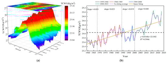
Figure 3.
(a) 3D plot of the monthly average change in global TCWV content from 1959–2023. (b) Trends in global annual mean TCWV content from 1959–2023.
3.1.2. Annual Anomalies and Cumulative Trends
Figure 4a shows the annual mean anomalies and cumulative anomaly changes of global TCWV from 1959 to 2023, highlighting phased trends in TCWV. The blue bars represent annual TCWV anomalies, indicating deviation from the long-term average, while the red line shows cumulative anomalies, reflecting interannual cumulative changes. The green dashed line represents the linear fit trend. Global TCWV cumulative anomalies initially declined, then increased. Before 2002, anomalies were mostly negative, indicating lower TCWV, while after 2002, anomalies remained positive, reflecting continuous TCWV growth, with 2002 as the turning point. Between 1976–1982 and 2003–2008, changes were small, indicating stable TCWV during these periods. To further confirm this trend, Figure 4b presents an analysis using the Mann–Kendall test. The Mann–Kendall test yielded a Z value of 6.708 (p < 0.001), with |Z| > 1.96, confirming statistical significance at the 0.05 level and indicating a significant long-term upward trend in TCWV. In Figure 4b, the UF curve shows a fluctuating decline before 1965, then a sharp rise, with a particularly sharp increase after 1976. From 1981 to 2023, the UF curve exceeded the ±0.05 threshold, indicating a significant upward mutation. The intersection of the UF and UB curves near 2004 suggests a mutation between 2002 and 2004, though the exact timing remains uncertain.
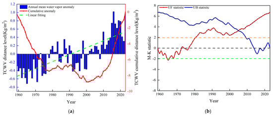
Figure 4.
(a) Analysis of cumulative distance level values of global annual TCWV content for 1959–2023. (b) Mann–Kendall trend test for global annual TCWV content, 1959–2023.
3.1.3. Mutation Analysis Using Sliding t-Test
To further identify the mutation points of TCWV, we performed an analysis using the sliding t-test method (Figure 5). Considering the timescales of TCWV variations and the periodic nature of climate events, we selected four sliding windows of 5, 7, 10, and 15 years to capture mutation characteristics at different timescales. The 5-year window detects short-term fluctuations (such as El Niño or La Niña events), the 7-year window corresponds to typical climate cycles (like ENSO), the 10-year window balances short-term fluctuations and long-term trends, and the 15-year window identifies prolonged climate patterns. The results showed multiple mutation instances under different windows: in the 5-year window, high-to-low mutations occurred in 1969, 1977–1980, 2002, 2009–2010, and 2012–2016, while low-to-high mutations were seen in 1991–1992 (Figure 5a); in the 7-year window, low-to-high mutations occurred in 1978–1979, 1991–1992, 2002–2003, 2010–2011, and 2015, with high-to-low mutations in 1976–1977, 2001–2002, 2009, and 2012–2014 (Figure 5b); in the 10-year window, low-to-high mutations occurred in 1973–1974, 1978–1981, 1991, 2003–2007, and 2011, while high-to-low mutations appeared in 1971–1972, 1975–1977, 1992, 2002, 2008–2009, and 2012 (Figure 5c); in the 15-year window, high-to-low mutations occurred in 1974–1977 and 2000–2008, while low-to-high mutations were observed in 1978–1981 (Figure 5d). Combining the Mann–Kendall trend analysis and sliding t-test, 2002 was identified as the year of a significant mutation from low to high, aligning with the El Niño-triggered global climate anomalies of that year. These changes underscore the key role of TCWV in regulating agricultural water resources and mitigating extreme weather risks, highlighting the need for adaptive land management strategies.
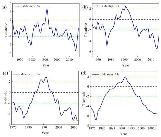
Figure 5.
Sliding t-test for global annual TCWV change, 1959-2023. (a) 5-year sliding t-test. (b) 10-year sliding t-test. (c) 7-year sliding t-test. (d) 15-year sliding t-test.
3.2. Spatial Variation Characteristics
3.2.1. Annual Spatial Dynamics and Five-Year Interval Spatial Trends
Figure 6 and Supplementary Figure S3 show the spatial dynamic characteristics of global TCWV from 1959 to 2023. Figure 6 indicates that the spatial pattern is consistent with the temporal trend of annual mean TCWV (Figure 3b), exhibiting phase characteristics: from 1959 to 1968, water vapor generally decreased; from 1968 to 1988, it significantly increased; from 1988 to 2000, there was an overall increase, but some regions experienced a decline; and from 2000 to 2023, there was a sharp rise. These phase fluctuations are closely related to the global climate context, such as the accelerated warming [51]. The increase in water vapor is particularly evident in the equatorial regions (e.g., the Amazon Basin, the Congo Basin, and Southeast Asia), where the annual increase has exceeded 2 kg/m2 since 2000, mainly due to enhanced convective activity in the tropical regions [7,52]. Supplementary Figure S3 further shows that the five-year variations were primarily fluctuating from 1959 to 1985, gradually increasing after the 1990s with the strengthening of the climate system, and accelerating notably after 2000, particularly in the tropics and monsoon regions (e.g., Southeast Asia, the Indian Ocean). These changes are mainly driven by global warming, with rising temperatures and accelerated water vapor circulation enhancing the atmospheric moisture capacity and convective activity [53]. Changes in atmospheric circulation have redistributed water vapor, increasing agricultural irrigation demands, impacting terrestrial ecosystems, and elevating flood risks.
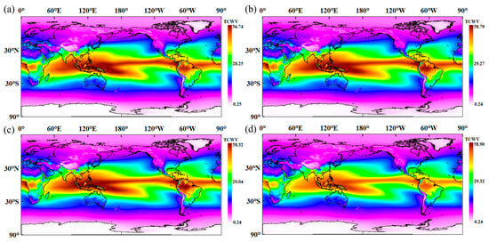
Figure 6.
Interannual spatial variation of TCWV, where the unit of TCWV is kg/m2. (a) Average interannual variation of TCWV from 1959 to 1968. (b) Average interannual variation of TCWV from 1968 to 1988. (c) Average interannual variation of TCWV from 1988 to 2000. (d) Average interannual variation of TCWV from 2000 to 2023.
3.2.2. Multi-Year Average Seasonal Distribution
Figure 7 illustrates the multi-year average seasonal distribution characteristics of global total column water vapor (TCWV) from 1959 to 2023, while Supplementary Table S2 lists the annual and seasonal mean values for each region. In Figure 7a, the global TCWV mean for spring is 17.478 kg/m2. Equatorial regions (e.g., the Amazon, Congo Basin, and Southeast Asia) exhibit higher water vapor content, approximately 25 kg/m2 (Supplementary Table S2a), benefiting from complex topography and intense convective activity, which supports the cultivation of high-yield crops such as rice and coffee, though flood risks must be monitored. Mid-to-high latitude regions (e.g., North America, Europe, and mid-latitude China) show relatively uniform water vapor distribution (15–20 kg/m2), conducive to stable agricultural production. Coastal regions (e.g., Japan and South Africa) experience significant seasonal water vapor fluctuations (difference of about 5 kg/m2), posing challenges to irrigation efficiency and pest control. Figure 7b shows that TCWV peaks in summer, with a mean of 20.334 kg/m2. Water vapor content in equatorial regions and surrounding Asian seas increases significantly, reaching a maximum of 68.251 kg/m2, with a notable increase compared to spring, but with extreme variability (minimum of only 0.123 kg/m2). While high water vapor content supports tropical agriculture, it markedly increases the risk of storms and extreme weather. In contrast, arid regions (e.g., North Africa and the Middle East) have water vapor content of only 8–10 kg/m2, making agriculture highly dependent on irrigation. In Figure 7c, autumn TCWV distribution is relatively balanced, with a mean of 17.305 kg/m2, a decrease of 3.029 kg/m2 from summer. High-latitude regions (e.g., the Arctic Circle) show minimal water vapor variation (difference < 2 kg/m2), suitable for developing precision agriculture to ensure stable crop yields. Figure 7d indicates that TCWV drops to its annual minimum in winter, with a mean of 17.009 kg/m2. Equatorial and tropical regions still have relatively high-water vapor content (maximum 57.830 kg/m2), while polar regions (e.g., Antarctica and the Arctic) have water vapor content below 5 kg/m2, forming a stark contrast and severely limiting agricultural development. Overall, global TCWV exhibits significant seasonal fluctuations, with a mean difference of 3.325 kg/m2 between summer and winter, an annual mean of 18.202 kg/m2, and an extreme value range from 0.251 kg/m2 to 68.251 kg/m2. The seasonal variation in equatorial regions is particularly pronounced, with summer water vapor increases far exceeding those in other regions, contrasting sharply with the stability of high-latitude areas.
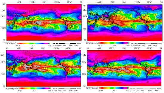
Figure 7.
Contour changes in global TCWV content averaged over different seasons, 1959-2023. (a) Spring TCWV changes. (b) Summer TCWV change. (c) Fall TCWV change. (d) Change in TCWV in winter.
3.2.3. Interannual Variation Rates
The global average interannual rate of change of TCWV calculated using the minimum pixel-scale trend is shown in Figure 8a–d. From 1959 to 2023, there is an overall increasing trend, particularly with significant rises in water vapor in Southeast Asia and surrounding seas, the Indian Ocean, tropical western Pacific, equatorial Africa, and the Amazon Basin in South America. In contrast, regions such as the Sahara Desert, central Australia, arid areas of Central Asia, and the southwestern United States exhibit a decreasing trend. In spring, the global increase is highest at 0.009 kg/m2/a (Figure 8a), followed by a peak of 0.015 kg/m2/a in summer (Figure 8b). In autumn, the increase falls back to 0.008 kg/m2/a (Figure 8c), and in winter, it remains steady at an annual average of 0.004 kg/m2/a (Figure 8d). The most dramatic humidity changes occur in summer, necessitating that agricultural production possess stronger adaptive capabilities to cope with extreme weather events, whereas in spring and winter, regional increases and decreases affect agricultural stability. These results indicate that TCWV distribution is closely associated with geographical location and climate patterns, confirming the characteristics of seasonal humidity distribution in the global climate and providing a scientific basis for agricultural water resource management and land use planning.
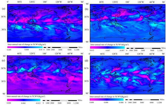
Figure 8.
1959-2023 average global interannual rates of change in TCWV for different seasons. (a) Spring interannual rate of change. (b) Summer interannual rate of change. (c) Fall interannual rate of change. (d) Winter interannual variability.
3.3. TCWV Prediction
3.3.1. Wavelet Transform Decomposition
Wavelet transform enables localized time-frequency analysis, overcoming limitations of single models in handling non-stationary, nonlinear TCWV data. Leveraging this, our study integrates wavelet transform with deep learning to develop a hybrid model aimed at enhancing TCWV prediction accuracy, supporting agricultural water resource management and land use decision-making. The modeling workflow is shown in Figure 9. The monthly mean TCWV data from 1959 to 2023 were preprocessed, and wavelet transform was used to decompose the nonlinear sequence into subsequences with different frequencies, reducing data complexity. During the wavelet transform process, the DB4 wavelet function was selected for a four-level decomposition, elevating the data from one-dimensional space to high-dimensional space, capturing TCWV variation trends, and enhancing model stability. The final decomposition, per Figure 10, resulted in five subsequences (A1, D1, D2, D3, D4), where A1 represents high-frequency rapid variation features, and D1–D4 represent low-frequency stable global trends. Analysis shows that the error between the wavelet-transformed data and the original data is only 6.699 × 10⁻⁸, proving that this method effectively restores the original data and ensures prediction accuracy.
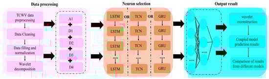
Figure 9.
Flowchart of wavelet transform coupled with different neural network models.
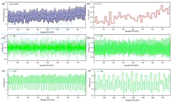
Figure 10.
Wavelet decomposition of TCWV data for 1959–2023. (a) Raw TCWV data. (b) A1 high-frequency data series. (c) D1 low-frequency data series. (d) D2 low-frequency data series. (e) D3 low-frequency data series. (f) D4 low-frequency data series.
Based on the decomposition results, deep learning models use the subsequences generated by wavelet transform (A1, D1, D2, D3, D4) as input, ensuring that the input data comprehensively covers TCWV variation features, making it suitable for predicting nonlinear and non-stationary time series. The input data were used to train LSTM, TCN, and GRU models. LSTM was selected for its ability to maintain long-term temporal dependencies, making it particularly suitable for analyzing the low-frequency trends (D1–D4) in water vapor variability. GRU, as an efficient variant of LSTM, balances performance and computational complexity, making it suitable for both high-frequency and low-frequency components (A1, D1–D4). TCN extracts multi-scale temporal features through dilated convolutions, providing a refined alternative to recurrent architectures and excelling at capturing dynamic changes. Traditional statistical models (e.g., ARIMA) and other neural networks (e.g., standalone CNNs or Transformers) were not used, as ARIMA cannot handle nonlinear multi-scale dynamics, CNNs lack adaptability for time-focused sequential data, and Transformers require extensive data and computational resources, which are not applicable given the temporal scope of this study.
By optimizing the network architecture and hyperparameters, the models’ ability to extract features and capture temporal dynamics was significantly enhanced. Predictions for each subsequence were derived from the testing set, and the final outputs of the WT-LSTM, WT-TCN, and WT-GRU models were generated through wavelet reconstruction. Each model was subjected to 10 iterations to ensure statistical stability. Finally, model evaluation metrics were compared to assess performance differences between the hybrid and single models in predicting monthly average TCWV content.
3.3.2. Model Prediction and Validation
The training process for the three neural network models was systematically configured to ensure reproducibility and robustness. The dataset was split into a training set (January 1959–December 2011, approximately 80%) and a testing set (January 2012–December 2023, approximately 20%), with 20% of the training data reserved for validation. Key hyperparameters were as follows: LSTM and GRU used two hidden layers with 128 and 64 units, respectively, a learning rate of 0.001, and a batch size of 32; TCN had three convolutional layers, each with 64 filters, a kernel size of 3, and dilation factors of [1,2,4], with the same learning rate and batch size. All models were trained for 100 epochs using the Adam optimizer to minimize Mean Squared Error (MSE), with early stopping after 10 epochs of no improvement to prevent overfitting. Dropout (rate of 0.2) was applied to LSTM and GRU, while TCN relied on regularization through dilated convolutions. Hyperparameter details are provided in Supplementary Table S3.
After completing the predictions using the three neural network models on the decomposed subsequences, Figure 11 presents a comparison between each model’s predicted values and actual observed values, while Table 1 provides detailed evaluation results (best performance highlighted in bold). Comprehensive analysis indicates that the TCN model achieves the best predictive performance on the D1 and D2 sequences, followed by the GRU model, while the LSTM model performs relatively weaker (Figure 11b,c). In the D3 sequence, TCN and GRU performance is comparable and slightly better than LSTM (Figure 11d). For the D4 and A1 decomposed sequences, the prediction performance of the three models is similar, with the coefficient of determination (R2) all close to 1, indicating that the models exhibit very high prediction accuracy for these sequences (Figure 11a,e).
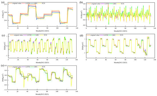
Figure 11.
Predictions of TCWV wavelet decomposition data for 1959-2023 from three different models. (a) A1 high-frequency data series prediction. (b) D1 low-frequency data series prediction. (c) D2 low-frequency data series prediction. (d) D3 low-frequency data series prediction. (e) D4 low-frequency data series prediction.

Table 1.
Results of evaluation metrics of LSTM, GRU, and TCN models for wavelet decomposition sequence prediction.
By performing wavelet reconstruction on the prediction results of each decomposed sequence, we ultimately obtained the overall prediction results of the coupled models. The predicted values of the wavelet-transform coupled models (WT-LSTM, WT-TCN, and WT-GRU) were systematically compared to the actual values. To fully evaluate their performance, we also compared the prediction results of single neural network models (LSTM, TCN, and GRU), ensuring consistency in settings and data division across both model types. Figure 12 illustrates the comparison of predicted curves for coupled and single models with actual measured values. Figure 12a shows that the WT-LSTM model has a small prediction error and accurately reflects data trends, especially showing high precision in predicting extreme points (peaks and troughs). In contrast, Figure 12b indicates that the single LSTM model has a larger prediction error in extreme areas (tops and bottoms), suggesting it is insufficient at capturing detailed variations in TCWV. Similarly, Figure 12c shows that the WT-GRU model effectively captures periodic changes in TCWV and performs excellently in predicting extreme points with smaller errors. However, as shown in Figure 12d, the single GRU model’s prediction error significantly increases in practical forecasting, especially in the latter half of the time series, indicating limited ability to handle complex changes. Figure 12e shows that the WT-TCN model’s prediction curve closely matches the actual measured values, demonstrating extremely high accuracy and stability in both overall trends and local details. In contrast, although the single TCN model in Figure 12f performs well in overall trends, it is still inferior to the WT-TCN model in detailed prediction.
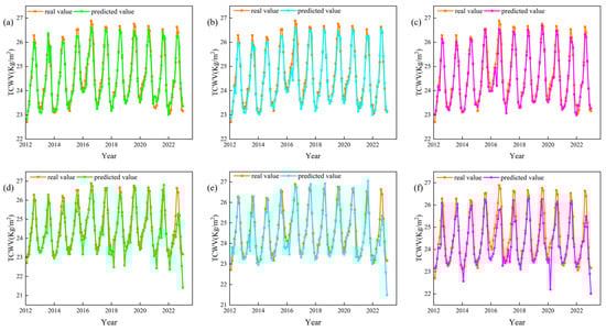
Figure 12.
Comparison of the prediction result curves for TCWV content between the coupled model and the single model. (a) WT-LSTM model prediction. (b) LSTM model predictions. (c) WT-GRU model prediction. (d) GRU model prediction. (e) WT-TCN model prediction. (f) TCN model prediction.
The scatter plots in Figure 13 further validate each model’s predictive performance. Figure 13a shows a highly linear relationship between the predicted values of the WT-LSTM model and the actual observed values, indicating the model’s excellent accuracy in TCWV prediction. In contrast, the single LSTM model in Figure 13b exhibits obvious deviations in prediction results, especially performing poorly in terms of lag and prediction accuracy. Specifically, the WT-LSTM model has a mean absolute error (MAE) of 0.195 and a coefficient of determination (R2) of 0.946, while the LSTM model has an MAE of 0.452 and R2 of 0.669, highlighting WT-LSTM’s significant advantage in overall predictive performance. Moreover, the WT-GRU model also demonstrates superior predictive capabilities. The scatter plot in Figure 13c shows a close linear relationship between WT-GRU’s predicted values and the actual values, with an MAE of 0.181 and R2 of 0.949, reflecting high prediction accuracy. However, the single GRU model in Figure 13d has an MAE of 0.499 and R2 of 0.615, showing that WT-GRU significantly improves prediction accuracy and response speed. Similarly, the WT-TCN model also exhibits outstanding predictive performance. The scatter plot in Figure 13e shows that the predicted values of the WT-TCN model highly match the actual measured values, with an MAE of 0.170 and R2 reaching 0.953, indicating that the model possesses the best accuracy and the lowest lag in TCWV content prediction. The single TCN model in Figure 13f has an MAE of 0.480 and R2 of 0.673; although its overall performance is acceptable, it is still inferior to WT-TCN in prediction accuracy and response speed. Detailed performance metrics for each model are provided in Table 2, with the best-performing model highlighted in bold.
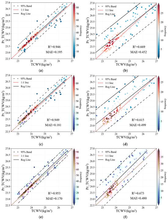
Figure 13.
Scatterplot comparison of coupled and single model predictions of TCWV content. (a) WT-LSTM model predictions. (b) LSTM model predictions. (c) WT-GRU model predictions. (d) GRU model prediction. (e) WT-TCN model prediction. (f) TCN model prediction.
Table 2.
Results of evaluation indicators for different forecasting models.
3.3.3. Comparison of Prediction Results
To further illustrate the performance of each model, Taylor diagrams (Figure 14) compare results based on standard deviation, correlation coefficient, and root mean square error. Figure 14a presents the results for single models, while Figure 14b shows the coupled models’ performance. The diagrams indicate that the points for the coupled models are closer to the reference circle, demonstrating higher correlation coefficients, standard deviations that are closer to the observed values, and smaller root mean square errors. These characteristics highlight the superiority of the coupled models over the single models in terms of prediction accuracy and stability. After comparing the prediction results of the three coupled models (WT-LSTM, WT-TCN, and WT-GRU) with the three single models (LSTM, TCN, and GRU), we found that the WT-TCN model most closely aligns with observed values. It outperformed both WT-GRU and WT-LSTM across all evaluation metrics. Specifically, compared to the WT-LSTM model, the WT-TCN model reduced MAE, RMSE, MSE, and MAPE by 12.82%, 6.20%, 12.12%, and 12.57%, respectively, while R2 increased by 0.74%. Compared to the WT-GRU model, the WT-TCN model showed improvements of 6.06%, 0.82%, 1.69%, and 5.88% in MAE, RMSE, MSE, and MAPE, respectively, with R2 increasing by 0.42%.
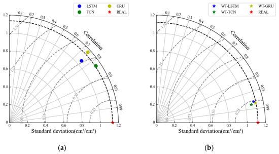
Figure 14.
Taylor diagram of the prediction results of the coupled model with wavelet variations compared to a single model. (a) Prediction results of the three single models. (b) Prediction results of three coupled models.
In addition, compared to their respective single models, all three coupled models show substantial improvements when using the single model as the baseline. For instance, the WT-GRU model reduced MAE, RMSE, MSE, and MAPE by 63.53%, 65.31%, 88.12%, and 63.47%, respectively, compared to the single GRU model, with R2 increasing by 54.34%. Similarly, the WT-TCN model reduced MAE, RMSE, MSE, and MAPE by 64.58%, 62.71%, 86.21%, and 64.02%, respectively, compared to the single TCN model, with R2 increasing by 41.65%. The WT-LSTM model, compared to the single LSTM model, reduced MAE, RMSE, MSE, and MAPE by 56.65%, 60.45%, 84.47%, and 56.47%, respectively, with R2 increasing by 41.48%. Detailed percentage improvements for each model can be found in Table 3, with the highest improvements highlighted in bold.
Table 3.
The percentage of improvement or decrease in various evaluation metrics of the coupled pre diction model compared to the single prediction model (%).
4. Discussion
4.1. The Spatiotemporal Variation Characteristics of TCWV
Through a detailed analysis of data from 1959 to 2023, this study elucidates the pronounced seasonal variations and long-term trends in global TCWV. Compared to previous studies primarily based on shorter time periods or satellite observations limited to specific regions [54,55], we utilize a 65-year global historical dataset, integrated with quantitative assessments of surface radiation and evaporation processes, to provide more precise quantifications of global TCWV seasonal fluctuations. Seasonal analysis reveals that TCWV exhibits significant periodic fluctuations. In summer, driven by intense solar radiation and evaporation, water vapor content reaches its annual peak, with a global mean of 20.334 kg/m2, particularly pronounced in equatorial and tropical regions (e.g., Southeast Asia and the tropical Pacific), where it reaches a maximum of 68.251 kg/m2 (Figure 3, Figure 6 and Figure 7). In winter, water vapor content is at its lowest, with a mean of 17.009 kg/m2, influenced by reduced radiation, resulting in a mean difference of 3.325 kg/m2 between summer and winter. The TCWV means for spring and autumn are approximately 17.478 kg/m2 and 17.305 kg/m2, respectively, with autumn showing a decrease of about 3.029 kg/m2 compared to summer. These seasonal patterns are consistent with the regulatory effects of solar radiation on atmospheric water vapor, as illustrated in the seasonal solar radiation maps for 1959–2023 (see Supplementary Figure S4). Compared to previous short-term analysis studies [54,55], this paper further quantifies the significant summer water vapor increase in equatorial regions and the smaller fluctuations in high-latitude regions (e.g., North America and the Arctic Circle, with differences < 2 kg/m2), and directly correlates this with the spatiotemporal heterogeneity of radiation changes.
Long-term trend analysis indicates that the global annual mean TCWV increases steadily at a rate of 0.0168 kg/m2/a, with a marked acceleration to 0.040 kg/m2/a after 2000, driven by enhanced evaporation, changes in atmospheric circulation, and global warming (see Figure 3, Figure 4 and Figure 5, Supplementary Figure S3 and Table S2). In key agricultural regions, such as Southeast Asia, the Indian Ocean, the tropical western Pacific, equatorial Africa, and the Amazon, water vapor content has significantly increased (e.g., a cumulative increase of 2 kg/m2 in the Amazon since 2000), exacerbating the frequency and intensity of extreme weather events (e.g., droughts, heavy rainfall, and floods) [56], posing a threat to land water resource stability. In contrast, mid-to-high latitude regions (e.g., North America and Europe, TCWV 15–20 kg/m2) exhibit relatively stable water vapor changes, while arid regions (e.g., North Africa and the Middle East, 8–10 kg/m2) and polar regions (e.g., Antarctica, <5 kg/m2) experience scarce water vapor, significantly increasing irrigation challenges [57]. In contrast to previous regional-scale studies [58], this paper, through global-scale analysis, elucidates the spatiotemporal variability of TCWV distribution driven by global warming, highlighting the stark contrast between substantial increases in tropical regions (up to 68.251 kg/m2) and low values in polar regions (<5 kg/m2), leading to uneven irrigation resource allocation, affecting crop growth and land use efficiency. Consequently, there is an urgent need to develop adaptive water resource and land management strategies to address the challenges of climate change to agricultural system sustainability [59].
4.2. Stability of Hybrid Model Predictions
Accurate prediction of TCWV changes is critical for addressing climate change impacts on agriculture, a priority underscored by advanced forecasting needs. Existing methods often combine remote sensing data, climate models, and machine learning to improve prediction accuracy [60]. Building on this, our study proposes a hybrid model integrating wavelet transform with neural networks (LSTM, TCN, GRU), leveraging wavelet decomposition of historical water vapor data to forecast future trends, thereby supporting irrigation management and land resource decision-making.
Comparative analysis of three hybrid models (WT-LSTM, WT-TCN, WT-GRU) and standalone models (LSTM, TCN, GRU) demonstrates that the WT-TCN model surpasses all others across all evaluation metrics, exhibiting strong consistency with observed data (see Figure 13 and Figure 14). In contrast to prior studies, such as Min et al. [61], who achieved an MAE of 0.07 mm and RMSE of 0.82 mm with the WLA model (wavelet transform coupled with LSTM-ARIMA) for GNSS precipitable water vapor prediction in a regional context, or Lu et al. [62], who reported an RMSE of 0.31 mm and MAE of 0.18 mm using the Light-PWV model for PWV forecasting in the Yangtze River Delta, our WT-TCN model advances global-scale forecasting. It achieves an MAE of 0.170 mm, an RMSE of 0.242 mm, and an R2 of 0.953, reflecting its robustness in capturing global water vapor trends. This study distinguishes itself by integrating wavelet transform with temporal convolutional networks, a novel approach that enhances feature extraction across multi-scale temporal patterns, surpassing the regional focus and methodological scope of previous models like WLA and Light-PWV. Although its MAE is slightly higher than some regional models, the WT-TCN’s low RMSE and high R2 highlight its superior stability and applicability for global predictions. Compared to standalone models as a benchmark, the hybrid models, particularly WT-TCN, reduce MAE (e.g., from 0.480 for standalone TCN to 0.170), RMSE, MSE, and MAPE, while increasing R2 to 0.953 (see Table 2 and Table 3). The WT-TCN’s exceptional performance stems from its ability to leverage wavelet decomposition for noise reduction and TCN’s dilated convolutions for capturing long-term dependencies, optimizing trend fitting and predictive accuracy for agricultural applications. While the WT-TCN model demonstrates considerable strengths, future changes such as carbon emission reductions and urban land use transformations may alter TCWV patterns, potentially impacting prediction accuracy. These external dynamics suggest the need for continued exploration in future studies to ensure robustness across diverse global conditions.
4.3. Impacts of TCWV Changes on Water Resource Management
The spatiotemporal distribution of TCWV directly impacts water resource management and utilization efficiency, a relationship well-established in hydro ecological research [63]. Through an in-depth analysis of water vapor dynamics conducted in this study, we show that such insights can contribute to optimizing irrigation strategies, enabling water resource managers to better address moisture variability and effectively mitigate risks associated with hydrological extremes such as droughts and floods. Furthermore, the water vapor variability trends identified in this study provide critical guidance for water resource planning, particularly in moisture-abundant regions, enhancing water use efficiency and ensuring long-term sustainability. Continuous monitoring of anomalous TCWV fluctuations strengthens early warning systems, supporting more proactive disaster prevention and response in water resource management.
Based on the distinct characteristics of TCWV variability across different regions, we propose regionalized water resource management strategies to enhance the resilience and sustainability of hydrological systems. Although TCWV analysis offers key insights into atmospheric humidity dynamics, it alone is insufficient for comprehensive decision-making, requiring integration with climate variables [64,65] such as temperature, precipitation, frost days, and drought indices to establish a robust policy foundation. In tropical and subtropical regions with high TCWV variability (e.g., the Amazon Basin and Southeast Asia), we recommend implementing flexible irrigation systems, water conservation techniques, and rainwater harvesting facilities, optimized with precipitation and temperature data, to mitigate the impacts of TCWV fluctuations on water resource demands, thereby improving water resource productivity and stability. In mid-to-high latitude regions with relatively stable TCWV levels (e.g., North America and Europe, TCWV 15–20 kg/m2), precision agriculture techniques are suitable, with irrigation schedules optimized based on frost day analysis to maximize water use efficiency and crop yields. In arid and polar regions with low TCWV content (e.g., North Africa, 8–10 kg/m2; Antarctica, <5 kg/m2), we suggest enhancing soil water retention capacity, developing drought-resistant crops (e.g., millet, sorghum) and flood-tolerant rice varieties, and formulating targeted policies informed by drought analysis to address harsh environmental conditions. The WT-TCN model predictions (MAE 0.170, R2 0.953) provide strong support for these strategies, enabling proactive crop selection and planting timing based on TCWV analysis, thereby enhancing hydrological system resilience, promoting sustainable water resource utilization, and ensuring food security, consistent with global sustainable development goals [66].
5. Conclusions
Total Column Water Vapor (TCWV) has a significant impact on water supply and productivity in agricultural land systems, and its spatiotemporal variation analysis and prediction provide critical insights for sustainable water resource management. This study systematically investigates the spatiotemporal variation characteristics and prediction potential of global TCWV from 1959 to 2023 using methods such as the Mann–Kendall test, sliding change point analysis, wavelet transform, and deep learning models. The results show that global total column water vapor (TCWV) exhibits a significant upward trend on both interannual and long-term (over 60 years) scales, with an average annual increase rate of 0.0168 kg/m2/a. A notable abrupt change occurred in 2002, intensifying interannual variability. Seasonal fluctuations are evident, with water vapor content peaking in summer (global mean of 20.334 kg/m2, maximum of 68.251 kg/m2 in tropical regions) and reaching its lowest in winter (global mean of 17.009 kg/m2). Water vapor variability is greater in tropical and subtropical regions, while mid-to-high latitude regions (15~20 kg/m2) remain relatively stable, and polar regions have the lowest water vapor content.
Furthermore, a new hybrid prediction model combining wavelet transform and deep learning has demonstrated notable advantages in TCWV forecasting. By training on historical data through deep learning, the model can more accurately predict future TCWV trends, providing support for addressing extreme weather events. The model evaluation results indicate substantial improvements in prediction stability and accuracy. Compared to independent models, the hybrid model’s coefficient of determination (R2) exceeds 0.940, the mean absolute error (MAE) is less than 0.180, the mean absolute percentage error (MAPE) is below 0.790, and the root mean square error (RMSE) is under 0.260. Among the models, the WT-TCN model performs the best, with MAE of 0.170, R2 of 0.953, MAPE of 0.687, and MSE of 0.058, showing its potential in addressing climate change uncertainty and supporting meteorological disaster warning systems.
Based on regional TCWV variations, targeted agricultural water management strategies are developed. In tropical regions (mean 25 kg/m2, summer maximum ~69 kg/m2), where a summer-winter difference of 3~4 kg/m2 triggers frequent monsoon rainfall, dynamic irrigation scheduling and advanced drainage systems mitigate flood risks, supporting high-yield crops like rice while optimizing planting timing. Mid- and high-latitude regions (15~20 kg/m2), with stable TCWV variations (difference < 2 kg/m2), can refine irrigation timing using soil moisture sensors and TCWV trends, enhancing crop resilience. Arid (8~10 kg/m2) and polar regions (<5 kg/m2) can adopt micro-irrigation and stress-adapted crops (e.g., millet, sorghum), leveraging TCWV predictions to optimize water use efficiency. These strategies maximize water vapor resources, guide equitable water allocation, and enhance agricultural resilience through proactive disaster mitigation and precision land planning.
Although this study has made significant progress, external variables such as accelerated urbanization, carbon emissions, and land use changes may affect the variation patterns of TCWV. Future research needs to further enhance the model’s adaptability to these dynamic factors and actively explore integrated AI model frameworks to more effectively capture the complex nonlinear patterns of water vapor dynamics, thereby improving prediction capabilities and providing stronger support for disaster mitigation and sustainable water resource management.
Supplementary Materials
The following supporting information can be downloaded at: https://www.mdpi.com/article/10.3390/hydrology12080206/s1, Figure S1 presents scatter plots and Taylor diagrams of site validation results in different regions. Figure S2 presents schematic diagrams of the three neural network model structures. Figure S3 illustrates the spatial variation of TCWV at five-year intervals from 1959 to 2023. Figure S4 shows the global seasonal mean surface solar radiation downward (SSRD) from ERA5 data (1959–2023). Table S1 lists detailed information on Total Column Water Vapor validation sites. Table S2 provides statistics of inter-annual and seasonal mean TCWV content changes (kg/m2) from 1959 to 2023. Table S3 provides detailed parameter configurations for each neural network model.
Author Contributions
L.X.: Conceptualization, Methodology, Software, Validation, Formal analysis, Investigation, Data curation, Writing—Original draft, Writing—Review and editing. K.M.: Conceptualization, Methodology, Formal analysis, Investigation, Data collection, Writing—original draft, Writing—review, Editing, Project management and Funding acquisition. Z.G., J.S. and S.M.B.: Investigation, Data Curation, and Resource Provision. Z.Y.: Resource & Editing. All authors have read and agreed to the published version of the manuscript.
Funding
This work was supported by the Central Public-interest Scientific Institution Basal Research Fund (No. Y2025YC86) and Key Project of Natural Science Foundation of Ningxia Department of Science and Technology (No. 2024AC02032).
Data Availability Statement
The ERA5 data used in this study, including monthly total column water vapor (TCWV) and solar radiation, are available from the Copernicus Climate Change Service (C3S) Climate Data Store (CDS) at https://cds.climate.copernicus.eu/ (accessed on 1 January 2025). The NCEP/NCAR reanalysis data, providing TCWV, and vertical profile observations from the NOAA Integrated Global Radiosonde Archive (IGRA), including temperature, humidity, and pressure, can be accessed via the NOAA National Centers for Environmental Information (NCEI) at https://www.ncei.noaa.gov/ (accessed on 1 January 2025) and https://www.ncei.noaa.gov/products/weather-balloon/integrated-global-radiosonde-archive (accessed on 3 January 2025), respectively.
Acknowledgments
We thank ECMWF for providing the ERA5 data and NOAA for supplying the IGRA data. We greatly appreciate the insightful comments and suggestions from the anonymous reviewers. This study did not use generative artificial intelligence (GenAI) tools to generate text, data, figures, or to assist in research design, data collection, analysis, or interpretation.
Conflicts of Interest
The authors declare that they have no known competing financial interests or personal relationships that could have appeared to influence the work reported in this paper.
References
- Lesk, C.; Rowhani, P.; Ramankutty, N. Influence of extreme weather disasters on global crop production. Nature 2016, 529, 84–87. [Google Scholar] [CrossRef]
- Minoli, S.; Jägermeyr, J.; Asseng, S.; Urfels, C.; Müller, C. Global crop yields can be lifted by timely adaptation of growing periods to climate change. Nat. Commun. 2022, 13, 7079. [Google Scholar] [CrossRef] [PubMed]
- Trenberth, K.E. Changes in precipitation with climate change. Clim. Res. 2011, 47, 123–138. [Google Scholar] [CrossRef]
- Johnson, S.E.A.; Ye, H.; Fetzer, E.J.; Li, J. Satellite-observed precipitation and total column water vapor. Front. Environ. Sci. 2024, 12, 1338678. [Google Scholar] [CrossRef]
- Wu, H.; Su, X.; Huang, S.; Singh, V.P.; Zhou, S.; Tan, X.; Hu, X. Decreasing dynamic predictability of global agricultural drought with warming climate. Nat. Clim. Change 2025, 15, 411–419. [Google Scholar] [CrossRef]
- Li, S.; Wu, L.; Wang, Y.; Geng, T.; Cai, W.; Gan, B.; Jing, Z.; Yang, Y. Intensified Atlantic multidecadal variability in a warming climate. Nat. Clim. Change 2025, 15, 293–300. [Google Scholar] [CrossRef]
- Wang, Z.; Lei, Y.; Che, H.; Wu, B.; Zhang, X. Aerosol forcing regulating recent decadal change of summer water vapor budget over the Tibetan Plateau. Nat. Commun. 2024, 15, 2233. [Google Scholar] [CrossRef]
- Tan, J.; Chen, B.; Wang, W.; Yu, W.K.; Dai, W. Evaluating Precipitable Water Vapor Products From Fengyun-4A Meteorological Satellite Using Radiosonde, GNSS, and ERA5 Data. IEEE Trans. Geosci. Remote Sens. 2022, 60, 4106512. [Google Scholar] [CrossRef]
- Peng, Y.; Addisu, H.; Fadwa, A.; Joseph, A.; Anna, K.; Felix, N.T.; Hansjörg, K. Feasibility of ERA5 integrated water vapor trends for climate change analysis in continental Europe: An evaluation with GPS (1994–2019) by considering statistical significance. Remote Sens. Environ. 2021, 260, 112416. [Google Scholar] [CrossRef]
- Dee, D.P.; Uppala, S.M.; Simmons, A.J.; Berrisford, P. The ERA-Interim reanalysis: Configuration and performance of the data assimilation system. Q. J. R. Meteorol. Soc. 2011, 137, 553–597. [Google Scholar] [CrossRef]
- Sasayama, T.; Okamura, N.; Higashino, K.; Yoshida, T. Improvement in magnetic nanoparticle tomography estimation accuracy by combining sLORETA and non-negative least squares methods. J. Magn. Magn. Mater. 2022, 563, 169953–169960. [Google Scholar] [CrossRef]
- You, Y.; Ting, M.; Biasutti, M. Climate warming contributes to the record-shattering 2022 Pakistan rainfall. npj Clim. Atmos. Sci. 2024, 7, 89. [Google Scholar] [CrossRef]
- Borger, C.; Beirle, S.; Wagner, T. Analysis of global trends of total column water vapour from multiple years of OMI observations. Atmos. Chem. Phys. 2022, 22, 10603–10621. [Google Scholar] [CrossRef]
- Kim, S.; Sharma, A.; Wasko, C. Nathan, RLinking Total Precipitable Water to Precipitation Extremes Globally. Earth’s Future 2022, 10, e2021EF002473. [Google Scholar] [CrossRef]
- Ayantobo, O.O.; Wei, J.; Kang, B.; Zhang, H. Spatial and temporal characteristics of atmospheric water vapour content and its relationship with precipitation conversion in China during 1980–2016. Int. J. Climatol. 2020, 40, 702–722. [Google Scholar] [CrossRef]
- Ren, D.; Wang, Y.; Wang, G.; Liu, L. Rising trends of global precipitable water vapor and its correlation with flood frequency. Geod. Geodyn. 2023, 14, 355–367. [Google Scholar] [CrossRef]
- Chhetri, M.; Kumar, S.; Pratim Roy, P.; Kim, B. Deep BLSTM-GRU model for monthly rainfall prediction: A case study of Simtokha, Bhutan. Remote Sens. 2020, 12, 3174. [Google Scholar] [CrossRef]
- Richardson, D.; Neal, R.; Dankers, R.; Mylne, K.; Cowling, R.; Clements, H.; Millard, J. Linking weather patterns to regional extreme precipitation for highlighting potential flood events in medium-to long-range forecasts. Meteorol. Appl. 2020, 27, e1944. [Google Scholar] [CrossRef]
- Zhang, X.; Zhou, Y.; Zhang, W.; Kou, M.; Li, B.; Dai, Y.; Yang, C. Water vapor content prediction based on neural network model selection and optimal fusion. J. Comput. Sci. 2024, 79, 102310. [Google Scholar] [CrossRef]
- Acito, N.; Diani, M.; Corsini, G. CWV-Net: A deep neural network for atmospheric column water vapor retrieval from hyperspectral VNIR data. IEEE Trans. Geosci. Remote Sens. 2020, 58, 8163–8175. [Google Scholar] [CrossRef]
- Chen, K.; Chen, K.; Wang, Q.; He, Z.; Hu, J.; He, J. Short-term load forecasting with deep residual networks. IEEE Trans. Smart Grid 2019, 10, 3943–3952. [Google Scholar] [CrossRef]
- Shi, X.; Li, T.; Wang, H.; Yeung, D.-Y.; Wong, W.K.; Woo, W.-C. Convolutional LSTM network: A machine learning approach for precipitation nowcasting. Adv. Neural Inf. Process. Syst. 2015, 28, 802–810. [Google Scholar] [CrossRef]
- Bai, S.; Kolter, J.Z.; Koltun, V. An empirical evaluation of generic convolutional and recurrent networks for sequence modeling. arXiv 2018, arXiv:1803.01271. [Google Scholar] [CrossRef]
- Zhang, H.; Xu, T.; Li, H.; Zhang, S.; Wang, X.; Huang, X. StackGAN: Text to photo-realistic image synthesis with stacked generative adversarial networks. In Proceedings of the IEEE International Conference on Computer Vision, Venice, Italy, 29 October 2017; pp. 5907–5915. [Google Scholar] [CrossRef]
- Xiao, C.; Chen, N.; Hu, C.; Wang, K.; Gong, J.; Chen, Z. Short and mid-term sea surface temperature prediction using time-series satellite data and LSTM-Adaboost combination approach. Remote Sens. Environ. 2019, 233, 111358. [Google Scholar] [CrossRef]
- Chen, R.; Wang, X.; Zhang, W.; Zhu, X.; Li, A.; Yang, C. A hybrid CNN-LSTM model for typhoon formation forecasting. Geoinformatica 2019, 23, 375–396. [Google Scholar] [CrossRef]
- Diouf, D.; Niang, A.; Thiria, S. Deep learning based multiple regression to predict total column water vapor (TCWV) from physical parameters in West Africa by using Keras library. Int. J. Data Min. Knowl. Manag. Process 2019, 9, 13–21. [Google Scholar] [CrossRef]
- Graham, R.M.; Hudson, S.R.; Maturilli, M. Improved performance of ERA5 in Arctic gateway relative to four global atmospheric reanalyses. Geophys. Res. Lett. 2019, 46, 6138–6147. [Google Scholar] [CrossRef]
- Hersbach, H.; Bell, B.; Berrisford, P.; Hirahara, S. The ERA5 global reanalysis. Q. J. R. Meteorol. Soc. 2020, 146, 1999–2049. [Google Scholar] [CrossRef]
- Durre, I.; Yin, X.; Vose, R.S.; Applequist, S.; Arnfield, J. Enhancing the Data Coverage in the Integrated Global Radiosonde Archive. J. Atmos. Ocean. Technol. 2018, 35, 1753–1770. [Google Scholar] [CrossRef]
- Liu, S.; Gong, P. Change of surface cover greenness in China between 2000 and 2010. Chin. Sci. Bull. 2012, 57, 1423–1434. [Google Scholar] [CrossRef]
- Mann, H.B. Nonparametric tests against trend. Econometrica 1945, 13, 245–259. [Google Scholar] [CrossRef]
- Topaloğlu, F.; Irvem, A.; Özfidaner, M. Re-evaluation of trends in annual streamflows of Turkish rivers for the period 1968–2007. Fresenius Environ. Bull. 2012, 21, 2043–2050. [Google Scholar]
- Yue, S.; Pilon, P. A comparison of the power of the t test, Mann-Kendall and bootstrap tests for trend detection. Hydrol. Sci. J. 2004, 49, 21–37. [Google Scholar] [CrossRef]
- Peng, J.; Chen, S.; Lü, H.; Liu, Y.; Wu, J. Spatiotemporal patterns of remotely sensed PM2.5 concentration in China from 1999 to 2011. Remote Sens. Environ. 2016, 174, 109–121. [Google Scholar] [CrossRef]
- Theil, H. A rank-invariant method of linear and polynomial regression analysis. Indag. Math. 1950, 12, 85–91. [Google Scholar] [CrossRef]
- Sen, P.K. Estimates of the regression coefficient based on Kendall’s tau. J. Am. Stat. Assoc. 1968, 63, 1379–1389. [Google Scholar] [CrossRef]
- Arts, L.P.A.; van den Broek, E.L. The fast continuous wavelet transformation (fCWT) for real-time, high-quality, noise-resistant time–frequency analysis. Nat. Comput. Sci. 2022, 2, 47–58. [Google Scholar] [CrossRef]
- Prokoph, A.; El Bilali, H. Cross-wavelet analysis: A tool for detection of relationships between paleoclimate proxy records. Math. Geosci. 2008, 40, 575–586. [Google Scholar] [CrossRef]
- Kisi, O. Wavelet regression model as an alternative to neural networks for river stage forecasting. Water Resour. Manag. 2011, 25, 579–600. [Google Scholar] [CrossRef]
- Mallat, S.G. A theory for multiresolution signal decomposition: The wavelet representation. IEEE Trans. Pattern Anal. Mach. Intell. 1989, 11, 674–693. [Google Scholar] [CrossRef]
- Hochreiter, S.; Schmidhuber, J. Long short-term memory. Neural Comput. 1997, 9, 1735–1780. [Google Scholar] [CrossRef]
- Cho, K.; Van Merriënboer, B.; Gulcehre, C.; Bahdanau, D.; Bougares, F.; Schwenk, H.; Bengio, Y. Learning phrase representations using RNN encoder-decoder for statistical machine translation. arXiv 2014, arXiv:1406.1078. [Google Scholar] [CrossRef]
- Shen, G.; Tan, Q.; Zhang, H.; Zeng, P.; Xu, J. Deep learning with gated recurrent unit networks for financial sequence predictions. Procedia Comput. Sci. 2018, 131, 895–903. [Google Scholar] [CrossRef]
- Rahul, G.D.; Harigovindan, V.P.; Rasheed, A.H.K.P.; Amrtha, B. Attention-driven LSTM and GRU deep learning techniques for precise water quality prediction in smart aquaculture. Aquac. Int. 2024, 32, 8455–8478. [Google Scholar] [CrossRef]
- Hewage, P.; Behera, A.; Trovati, M.; Pereira, E.; Ghahremani, M.; Palmier, F.; Liu, Y. Temporal convolutional neural (TCN) network for an effective weather forecasting using time-series data from the local weather station. Soft Comput. 2020, 24, 16453–16482. [Google Scholar] [CrossRef]
- Liu, S.; Xu, T.; Du, X.; Zhang, Y.; Wu, J. A hybrid deep learning model based on parallel architecture TCN-LSTM with Savitzky-Golay filter for wind power prediction. Energy Convers. Manag. 2024, 302, 118122. [Google Scholar] [CrossRef]
- Zheng, Y.; Lu, C.; Wu, Z.; Liao, J.; Zhang, Y.; Wang, Q. Machine learning-based model for real-time GNSS precipitable water vapor sensing. Geophys. Res. Lett. 2022, 49, e2021GL096408. [Google Scholar] [CrossRef]
- Huang, L.; Peng, H.; Liu, L.; Xiong, S.; Xie, S.; Chen, J.; Li, H.; He, H. GNSS precipitable water vapor retrieval with the aid of NWM data for China. Earth Space Sci. 2021, 8, e2020EA001550. [Google Scholar] [CrossRef]
- Kim, S.; Shin, J.-Y.; Lee, G.; Park, J.; Sung, K. Future changes in precipitation extremes over South Korea based on observations and CMIP6 SSP scenarios. Water 2025, 17, 1702. [Google Scholar] [CrossRef]
- IPCC. Climate Change 2023: Synthesis Report; Intergovernmental Panel on Climate Change: Geneva, Switzerland, 2023; pp. 1–85. Available online: https://www.ipcc.ch/report/ar6/syr/ (accessed on 5 May 2025).
- He, C.; Wang, Z.; Zhou, T.; Li, T. Enhanced Latent Heating over the Tibetan Plateau as a Key to the Enhanced East Asian Summer Monsoon Circulation under a Warming Climate. J. Clim. 2019, 32, 3373–3388. [Google Scholar] [CrossRef]
- Liu, Y.; Fang, J.; Mu, S. Evaluation and future projection of compound extreme events in China using CMIP6 models. Clim. Change 2025, 178, 11. [Google Scholar] [CrossRef]
- Trenberth, K.E. The changing flow of energy through the climate system. J. Clim. 2020, 33, 5187–5202. [Google Scholar] [CrossRef]
- IPCC. Climate Change 2021: The Physical Science Basis; Cambridge University Press: Cambridge, UK, 2021. [Google Scholar] [CrossRef]
- Zelinka, M.D.; Myers, T.A.; McCoy, D.T.; Po-Chedley, S.; Caldwell, P.M.; Ceppi, P.; Klein, S.A.; Taylor, K.E. Causes of higher climate sensitivity in CMIP6 models. Geophys. Res. Lett. 2020, 47, e2019GL085782. [Google Scholar] [CrossRef]
- Huang, B.; Menne, M.J.; Boyer, T.; Freeman, E.; Gleason, B.E.; Lawrimore, J.H.; Liu, C.; Rennie, J.J.; Schreck, C.J.; Yang, F.; et al. Uncertainty estimates for sea surface temperature and land surface air temperature in NOAAGlobalTemp version 5. J. Clim. 2020, 33, 1351–1379. [Google Scholar] [CrossRef]
- World Meteorological Organization (WMO). State of the Global Climate 2023; WMO Report: Geneva, Switzerland, 2023; pp. 1–84. Available online: https://library.wmo.int/idurl/4/68236 (accessed on 1 May 2025).
- Lobell, D.B.; Schlenker, W.; Costa-Roberts, J. Climate trends and global crop production since 1980. Science 2011, 333, 616–620. [Google Scholar] [CrossRef] [PubMed]
- Sukanya, S.; Joseph, S. Climate change impacts on water resources: An overview. Vis. Tech. Clim. Change Mach. Learn. Artif. Intell. 2023, 4, 55–76. [Google Scholar] [CrossRef]
- Shangguan, M.; Dang, M.; Yue, Y.; Zou, R. A combined model to predict GNSS precipitable water vapor based on deep learning. IEEE J. Sel. Top. Appl. Earth Obs. Remote Sens. 2023, 16, 4713–4723. [Google Scholar] [CrossRef]
- Lu, H.X.; Li, K.; Li, L.; He, Q.; Yu, H.; Dong, Z. Research on precipitable water vapor prediction method based on LightGBM algorithm. GNSS World China 2024, 49, 110–119. [Google Scholar] [CrossRef]
- Piao, S.; Ciais, P.; Huang, Y.; Shen, Z.; Peng, S.; Li, S.; Zhou, L.; Liu, H.; Ma, Y.; Ding, Y.; et al. The impacts of climate change on water resources and agriculture in China. Nature 2010, 467, 43–51. [Google Scholar] [CrossRef]
- Handoko, E.Y.; Syariz, M.A.; Hanansyah, M.P.; Kuryawati, P.; Wijayanti, R.F.; Karondia, L.A. Assessing drought related to global climate phenomena using Sentinel-3 SLSTR data around East Java, Indonesia. Res. Sq. 2025, 1–20. [Google Scholar] [CrossRef]
- Musyimi, P.K.; Sahbeni, G.; Timár, G.; Weidinger, T.; Székely, B. Analysis of short-term drought episodes using Sentinel-3 SLSTR data under a semi-arid climate in Lower Eastern Kenya. Remote Sens. 2023, 15, 3041. [Google Scholar] [CrossRef]
- Vörösmarty, C.J.; Green, P.; Salisbury, J.; Lammers, R.B. Global water resources: Vulnerability from climate change and population growth. Science 2000, 289, 284–288. [Google Scholar] [CrossRef] [PubMed]
Disclaimer/Publisher’s Note: The statements, opinions and data contained in all publications are solely those of the individual author(s) and contributor(s) and not of MDPI and/or the editor(s). MDPI and/or the editor(s) disclaim responsibility for any injury to people or property resulting from any ideas, methods, instructions or products referred to in the content. |
© 2025 by the authors. Licensee MDPI, Basel, Switzerland. This article is an open access article distributed under the terms and conditions of the Creative Commons Attribution (CC BY) license (https://creativecommons.org/licenses/by/4.0/).