Abstract
The present study explores the application of RNNs for the prediction and propagation of flood waves along a section of the Bârsa River, Romania, as a fast alternative to classical hydraulic models, aiming to identify new ways to alert the population. Five neural architectures were analyzed as follows: S-RNN, LSTM, GRU, Bi-LSTM, and Bi-GRU. The input data for the neural networks were derived from 2D hydraulic simulations conducted using HEC-RAS software, which provided the necessary training data for the models. It should be mentioned that the input data for the hydraulic model are synthetic hydrographs, derived from the statistical processing of recorded floods. Performance evaluation was based on standard metrics such as NSE, MSE, and RMSE. The results indicate that all studied networks performed well, with NSE and values close to 1, thus validating their capacity to reproduce complex hydrological dynamics. Overall, all models yielded satisfactory results, making them useful tools particularly the GRU and Bi-GRU architectures, which showed the most balanced behavior, delivering low errors and high stability in predicting peak discharge, water level, and flood wave volume. The GRU and Bi-GRU networks yielded the best performance, with RMSE values below 1.45, MAE under 0.3, and volume errors typically under 3%. On the other hand, LSTM architecture exhibited the most significant instability and errors, especially in estimating the flood wave volume, often having errors exceeding 9% in some sections. The study concludes by identifying several limitations, including the heavy reliance on synthetic data and its local applicability, while also proposing solutions for future analyses, such as the integration of real-world data and the expansion of the methodology to diverse river basins thus providing greater significance to RNN models. The final conclusions highlight that RNNs are powerful tools in flood risk management, contributing to the development of fast and efficient early warning systems for extreme hydrological and meteorological events.
1. Introduction
In recent years, the climatic context has clearly shown an increase in both the frequency and severity [1] of extreme hydrological events [2], primarily driven by the adverse effects of climate change and land use dynamics [3]. These events pose a major risk to both human safety and infrastructure, whether referring to hydrotechnical or civil infrastructure. This is particularly critical in mountainous river basins where response time is limited. Consequently, the growing demand for rapid and accurate flood forecasting solutions, especially under constrained computational resources, has become a high priority in hydrological research. This makes the integration of artificial intelligence-based techniques highly relevant.
Classical hydraulic modeling tools such as HEC-RAS [4], MIKE 21 [5], or IBER [6] provide a very solid foundation for simulating flood wave effects; however, their main drawbacks include high computational time and a significant requirement for input data and user expertise. This makes them less suitable for real-time forecasting or for scenarios that require rapid decision-making. As a result, there is a growing need for a hybrid or fully data-driven method capable of capturing hydraulic behavior through machine learning.
In parallel, the rapid global development of deep learning technologies [7], particularly those based on recurrent neural networks (RNNs) [8], has recently opened new perspectives for hydrological applications [9]. These technologies have immense potential for reducing operational complexity and significantly decreasing the time required for flood wave prediction and propagation, starting from a well-defined dataset and set of assumptions.
RNNs are a special type of artificial neural network [10], with architectures specifically designed to process sequential data and capable of learning complex temporal relationships, making them ideal for analyzing the propagation and forecasting of discharge and water level time series [11,12]. Due to their internal memory and recursive structure, two of their main advantages, these models can capture the dynamic and time varying shape of the flood wave [13] and simulate the behavior of the entire hydraulic system based on past conditions (training).
According to the specialized literature, both RNNs [14] and their improved variants such as Long Short-Term Memory (LSTM) [15] and Gated Recurrent Unit (GRU) [16] have been applied to various problems, including water level forecasting [17], discharge prediction at different points along rivers [18], precipitation forecasting [19], runoff modeling, and hydrological risk assessment. However, artificial intelligence applications designed to replicate the propagation of flood waves compared to specialized hydraulic modeling software remain limited, particularly due to the lack of rigorous comparative methods and methodologies.
This paper aims to analyze a methodology based on prediction and modeling the hydraulic evolution of a flood wave synthetically generated and previously unknown to the neural networks over a short river segment of approximately 11.5 km. The selected river sector is the Bârsa River, a tributary of the Olt River in Romania [20]. The study seeks to assess the potential of five types of recurrent neural networks—S-RNN, LSTM, GRU, Bi-LSTM, and Bi-GRU [21]—in terms of their ability to simulate flood wave propagation, free surface water level, and flood wave volume [22,23]. Unlike other studies, this approach is rooted in a 2D hydraulic model developed using HEC-RAS software, with the results from the hydraulic simulations serving as training data for the neural networks. The goal of this approach is to translate knowledge from deterministic physical modeling [24] into the space of neural modeling, with the primary objective of evaluating the capacity of RNNs to understand and replicate hydraulic behavior along a well-studied river segment.
Following the tests, the GRU and Bi-GRU networks demonstrated the highest accuracy in replicating the shape of the flood wave, with RMSE values below 1.45 and volume errors under 3% in most of the analyzed sections. LSTM, on the other hand, showed weaker performance in some cases, with volume errors exceeding 9%, particularly in downstream areas near confluences.
To validate the simulated results, the network predictions are compared both globally (across 22 evenly distributed cross-sections selected at key points along the river) and locally, in two representative sections located downstream of confluences with other rivers. To enhance confidence in the simulated outcomes, model evaluation was performed using standard hydrological metrics [25], such as Nash–Sutcliffe Efficiency (NSE), the Coefficient of Determination (), Mean Squared Error (MSE), Root Mean Squared Error (RMSE), and Mean Absolute Error (MAE).
The values obtained for NSE and ere consistently close to 1, confirming the fidelity of the neural network simulations in relation to the data generated with HEC-RAS. Additionally,, the networks demonstrated good stability in maintaining the general shape of the hydrographs and accurately estimating peak discharges.
Moreover, the results obtained in this study demonstrate the potential to directly influence both engineering practice and flood risk management policy by offering a fast and automated alternative to classical hydraulic simulations. The integration of recurrent neural networks into the process of flood wave forecasting and propagation [26], as well as in determining water surface levels along river segments, could enable local flood risk management authorities to generate real-time predictions of water level and discharge at key points within the hydrographic network particularly in areas known to have a high flood risk [27]. The main advantage is that it eliminates the need to run full-scale hydraulic models after the neural networks have been trained. This result is particularly valuable in emergency situations, where reaction time is critical and running a full physical model may become unfeasible due to limited resources or time constraints.
In the scientific literature, most studies based on recurrent neural networks (RNNs) applied to hydrology focus on streamflow forecasting at a single control point [8,11] or on estimating the peak value of a flood wave [22,23]. Moreover, many of these studies do not test the ability of RNNs to reproduce an entire spatial–temporal flood wave propagation process, as classical physical models like HEC-RAS or MIKE do.
Thus, a significant knowledge gap emerges as follows: can an RNN-based model fully replace a hydraulic solver within a river reach, using only upstream information and synthetic data, without access to the explicit geometry of the riverbed?
The present study aims to address this question by evaluating the performance of five recurrent neural network architectures (Simple RNN, LSTM, Bi-LSTM, GRU, and Bi-GRU), trained on the outputs of a 2D HEC-RAS hydraulic model. The main objectives are to test the ability of these networks to reproduce the shape of the flood wave along the entire river section, across multiple cross-sections; and to identify the optimal architecture for potential operational deployment.
The novelty of this study lies in its holistic approach to flood wave propagation, treating it not merely as a pointwise problem but as a spatial–temporal sequence, thus contributing significantly to the integration of AI into hydraulic modeling. Moreover, the use of synthetic yet realistic data enables a controlled and reproducible validation of the proposed methods.
Given the need for efficient emergency management such as flood warnings or rapid post-event assessments, this method could become a valuable tool for both those responsible for managing hydrotechnical infrastructure and the authorities in charge of emergency response [28]. Thus, the present study offers both a theoretical and practical contribution, supported by the analyzed case study, demonstrating its immediate relevance to modern strategies for adapting to extreme hydrometeorological phenomena caused by climate change.
The conclusions support the potential of integrating recurrent neural networks into early warning systems, drastically reducing computational costs and enabling real-time operational forecasting. The study also has several limitations, outlined as follows: the use of synthetic data excludes unforeseen influences present in real-world datasets (such as measurement errors or atypical flood behaviors), and extending the approach to other catchments requires a new training phase, which limits the direct generalization of the trained networks.
2. Materials and Methods
2.1. Study Area
The Bârsa River (cadastral code 08.01.050) is one of the most important tributaries within the upper hydrographic basin of the Olt River (cadastral code 08.01), with their confluence occurring near the locality of Feldioara.
Significant for the Transylvanian region of Romania, the Bârsa River extends over 73 km, encompassing a hydrographic basin area of 937 km2, and it crosses major localities, notably, the Brașov Municipality and the town of Zărnești [29].
The current paper focuses on the upper hydrographic basin of the Bârsa River, specifically analyzing an approximately 11.5 km-long section (Figure 1). This chosen area is located roughly 12 km downstream from the river’s source and is characterized by two significant left-bank tributaries (Bârsa lui Bucur River and Bârsa Fierului River), which play a crucial role in the hydrology of the main river.
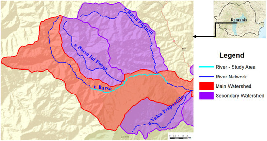
Figure 1.
Bârsa river—study area.
2.2. Data
The maximum discharge values were calculated based on a detailed analysis of historical information regarding the runoff regime of the Bârsa River. Given that the basin area, within the context of the current study, is less than 100 km2, genetic calculation formulas were employed to determine the maximum discharge, in accordance with the current methodology [30,31]. These formulas rely on the maximum rainfall intensity corresponding to a 1% probability, as well as the runoff coefficient, assessed according to basin slope, land use patterns, and vegetation cover. Calculations were performed by the National Institute of Hydrology and Water Management (INHGA) within the framework of the project “Flood Hazard and Flood Risk Maps and Flood Risk Management Plans for Romania” [32] and were provided by S.C. AQUAPROIECT S.A.
Synthetic hydrographs determined at three key points along the configuration of the Bârsa River were used as input data. As illustrated in Figure 2, the data were provided at the starting point of the analysis (start point) and at the confluence of the Bârsa River with its tributaries, Bârsa lui Bucur River and Bârsa Fierului River (conf. points). Flow values were delivered both upstream and downstream of the confluence, thus allowing the exact contribution of the inflows to be determined.
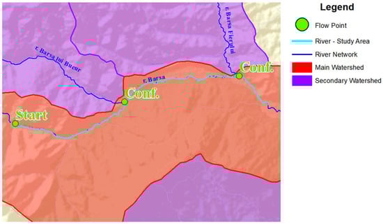
Figure 2.
Bârsa river—available data.
At each of the three input points, seven synthetic hydrographs were determined, for annual exceedance probabilities of 0.1%, 0.2%, 0.5%, 1%, 1%CC, 10%, and 33%, respectively. The hydraulic hypothesis adopted along the river assumed a constant annual exceedance probability throughout its length (Figure 3).
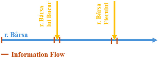
Figure 3.
Topological scheme of Bârsa river—study area.
To fulfill this hydraulic hypothesis, discharge corrections were applied at the confluence zones, accompanied by uniformly distributed lateral inflows along the river’s length.
Hydraulic Modeling
The adopted hydraulic hypothesis was fulfilled through flood wave propagation using hydraulic modeling software HEC-RAS (Hydrologic Engineering Center’s River Analysis System), version 6.6, developed by the US Army Corps of Engineers Hydrologic Engineering Center [33]. For this purpose, a fully 2D hydraulic model was built (Figure 4), incorporating over 119,000 computational cells, with a resolution of 15 m2 in the floodplain area and a higher resolution of 5 m2 within the main riverbed and near features that may influence flow (embankments, roads, or bridges).
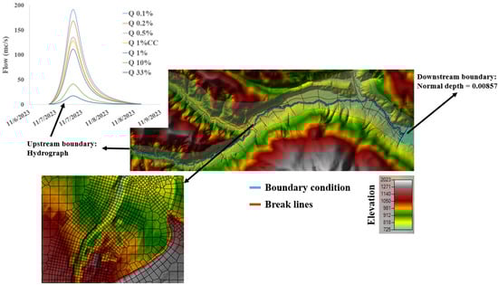
Figure 4.
Schematization of the hydraulic model and the calculation area—river Bârsa—HEC-Ras—version 6.6.
The hydraulic modeling was performed for all seven synthetic hydrographs calculated (annual exceedance probabilities of 0.1%, 0.2%, 0.5%, 1% CC, 1%, 10%, and 33%). Calculations were based on the Digital Terrain Model (DTM), into which measured topo-bathymetric cross-sections along the river were integrated [34,35]. In addition to the DTM, the model considered the land cover types present in the area. Thus, roughness coefficients (Figure 5) were sourced from the specialized literature (Table 1) [36] and distributed according to land cover types, facilitated by the freely available European Union resource, Corine Land Cover [37].
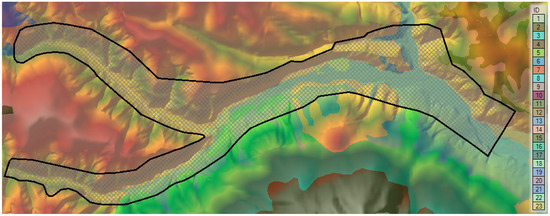
Figure 5.
Roughness distribution.

Table 1.
Roughness coefficient (Manning’s).
Another important element, addressed with utmost seriousness, was the stability of the model, achieved using the Courant number (Courant–Friedrichs–Lewy—CFL).
The CFL number is a dimensionless parameter used as a necessary condition for convergence in the numerical solution of certain partial differential equations (especially hyperbolic equations) [38].
where v—propagation velocity (e.g., water velocity); ∆t—time step; ∆x—spatial step (length of a computational cell).
It appears in the numerical analysis of explicit time integration schemes when these are used for numerical solutions. Consequently, the time step must be smaller than some upper bound, given a fixed spatial increment, in many computer simulations with explicit time displacement; otherwise, the simulation produces incorrect or unstable results [39].
If the CFL value is less than 1, the numerical solution is considered stable (a necessary condition, but not always sufficient). Conversely, if the CFE value is greater than 1, the solution is considered numerically unstable, thus changing the time step.
This parameter is fundamental in hydraulic modeling, based on the relationship between the physical propagation velocity of the flood wave and the ratio between the time step and computational cell size. Maintaining the Courant number within a specific interval ensures the numerical stability of the model and minimizes volume and water level errors in mathematical modeling. The present study established upper and lower limits of 2 and 0.7, respectively, enhancing model stability and thereby the quality of results [40]. Setting the upper limit to a relatively low number may increase simulation time but ensures calculations of high accuracy, which was desired for this study.
The summarized results presented in Table 2, obtained after adjusting the model stability and applying a variable time step based on the Courant number, indicate a high degree of quality for the resulting hydraulic outputs, thus enhancing the reliability of the data obtained. If we look at the percentage error, we observe an increasing trend from AEP 0.2% to AEP 10% although the increase is low. The explanation is related to the fact that for higher APE, the model has the calculation cells filled with water, while for lower AEP, they start to be empty; thus, the model needs more iterations to stabilize.
Table 2.
Centralizing table—stability and time of the hydraulic model.
2.3. Model Evaluation Metrics
Regarding the evaluation of the performance of the recurrent neural networks employed, several metrics specifically used in time-series processing were selected, precisely matching the context of the discharge and water level hydrographs that formed the basis for training and testing the neural networks.
The Mean Squared Error (MSE) is the first metric used to analyze the competence of the model and is defined by Equation (2) [41].
where represents the data simulated by the neural network, and represents the data used for training. MSE quantifies the mean of squared errors between the observed (real) and predicted values by the network.
where RMSE (Root Mean Squared Error) is the square root of the MSE, offering the advantage of returning precise values measured in the same units as the training data, thus being easier to interpret [42].
Other metrics are the MAE Equation (4), Equation (5), and NSE Equation (6).
where MAE (Mean Absolute Error) represents the mean of the absolute values of the errors, with denoting the values simulated by the network and d the training data [43]. The main advantage of this metric is that it does not overemphasize peak values, making it more realistic in low-flow or low altitude regions.
Taking a step further, in order to enhance confidence in the quality of model training, several more robust metrics were also employed, such as the Coefficient of Determination [44], which is based on the Pearson correlation, expressed as follows:
The coefficient offers several advantages, including its ability to purely capture the correlation between simulated and observed values, as well as its independence from systematic bias.
In addition to , the Nash–Sutcliffe Efficiency (NSE) metric was also employed. NSE is a fundamental performance metric in hydrology, as it evaluates the model’s ability to reproduce the dynamics of observed values based on the simulated data [45].
Given the suitability of and NSE for hydrological tasks, these metrics were considered key elements in evaluating the performance of the recurrent neural network prediction models [46,47,48]. By using these metrics, a more reliable and detailed assessment is provided compared to traditional metrics. This approach enables a more nuanced evaluation of model performance, accounting for the inherent complexity of hydrological modeling.
2.4. Recurrent Neuronal Networks
Recurrent Neural Networks (RNNs) are a class of more advanced Artificial Neural Networks (ANNs), with their main advantage being the ability to model sequential data characterized by temporal dependencies [49]. This feature is essential in the analysis of hydrological data, which change their characteristics over time.
Another key feature of RNNs lies in their recurrent connections, which allow information to be reused in successive stages of the learning process [50]. As a result, these models are capable of capturing dynamic relationships and temporal contexts within time series.
Due to their specific architecture [51], RNNs are highly effective in identifying complex patterns, particularly in large volumes of data, and are very capable of forecasting future values, making them extremely useful across various application domains.
In the present article, five different RNNs were analyzed, each with distinct configurations. The objective was to identify the optimal training approach based on the available data and to determine the method that yields the best performance.
2.4.1. Simple Recurrent Neuronal Networks
Simple Recurrent Neural Networks (S-RNNs) represent the most fundamental and basic form of RNNs, characterized by the recurrent connection between layers. The key distinction between this type of network and traditional feedforward neural networks lies in the ability of S-RNNs to use the hidden state from a previous time step as part of the current input, thereby enabling short-term memory of past information within analyzed data sequences.
Although their simple architecture offers advantages in terms of implementation and interpretability, S-RNNs can encounter significant challenges when it comes to retaining long-term information. Nevertheless, they can be a suitable choice for modeling data with short-term temporal dependencies.
The fundamental equations that describe the functioning of S-RNNs are as follows [52]:
where —hidden state; —output vector; —input vector at time t; —previous layer (recurrence); ; —matrix of weights associated with the inputs; —the bias vector associated with the hidden layer; —the activation function; —the matrix of hidden weights in the output layer; and —the bias associated with the output.
2.4.2. Long Short-Term Memory
Long Short-Term Memory (LSTM) neural networks are a more advanced and specialized variant of recurrent neural networks, specifically designed to address the vanishing gradient problem and to enhance the ability to capture long-term temporal dependencies in data sequences. Hochreiter and Schmidhuber [53] are the originators of this type of network, which has since undergone various improvements that have further increased its capabilities [54].
The main advantage of LSTM over classical RNNs lies in the use of internal structures called gates and memory cells, which can store information over extended periods of time [55]. The LSTM architecture is built on three fundamental components: the cell state, representing long-term memory; the hidden state, which captures the output from the previous time step; and the input data from the current time step [56].
Through its gating mechanisms, the LSTM can selectively decide what information to retain, what to forget, and what to pass on, enabling the network to memorize complex long-term relationships. These states are defined by the following equations.
where , , and are the values of the forget gates, input gates, and output gates at time step t. s a sigmoid activation function, is the candidate cell state value, and are weighted matrices, and represents element-wise multiplication.
2.4.3. Gated Recurrent Unit
Gated Recurrent Units (GRUs) are a simplified yet highly effective variant of LSTM networks. They were introduced to retain the advantages of LSTM models while adopting similar architecture [57]. The main difference between the two lies in the number of internal gates as follows: while LSTMs use three gates, the GRU model uses only two—update and reset gates.
The update gate determines how much of the previous information should be carried forward, whereas the reset gate decides how much of the past information should be forgotten or retained.
Both GRU and LSTM models excel at managing long-term sequential dependencies; however, the key distinction is that GRUs achieve this with a simpler, more efficient architecture, making them a preferred choice in many cases [58].
In GRU architecture, the output of the memory cell () at time step t serves both as the input for the next computation and as the basis for decision-making. The equations that define these values are the following:
2.4.4. Bidirectional Long Short-Term Memory
Bidirectional Long Short-Term Memory (Bi-LSTM) recurrent neural networks are a powerful extension of classical LSTM networks, with the ability to capture both past and future dependencies in sequential datasets [59]. The fundamental difference from standard LSTMs, which process data in a single direction (typically forward), is that Bi-LSTMs have two LSTM layers that analyze the data in opposite directions [60]. The first layer processes the input sequence from start to end, while the second layer processes the sequence from end to start.
The combined output of these two LSTM networks allows for the extraction of more complex sequence representations, which increases both the complexity and performance of the network. The final output is a combination of the forward and backward sequences, often through concatenation, making Bi-LSTMs particularly useful for tasks that require sequential context.
2.4.5. Bidirectional Gated Recurrent Unit
Similarly to Bi-LSTM networks, Bidirectional Gated Recurrent Unit (Bi-GRU) networks have the ability to process sequential information in both the forward (from start to end) and backward (from end to start) directions [61]. Their underlying architecture is similar to that of Bi-LSTM networks, incorporating the general characteristics of GRUs [62].
This dual approach enables the modeling of global temporal contexts, allowing the network to take into account both past and future information relative to a given point in a sequence.
2.5. Methods
For the present study, the deep learning models (S-RNN, LSTM, GRU, Bi-LSTM, Bi-GRU) [63] were developed using free Python software (version 3.12.0). In addition to Python, the working environment was built using the TensorFlow package (version 2.16.1) and Keras (version 3.3.3), all of which are open source [64,65].
The workflow diagram is presented in Figure 6. The process is divided into four major successive stages, each with a different level of complexity.
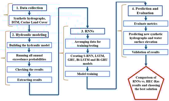
Figure 6.
Procedural workflow diagram.
The first stage involves the collection of input data required for hydraulic modeling. This includes synthetic discharge hydrographs for various annual exceedance probabilities, the Digital Terrain Model (DTM), land use information (Corine Land Cover), as well as existing hydrotechnical and road infrastructure.
The second stage of the workflow consists of performing hydraulic modeling, starting from building the hydraulic model using HEC-RAS software, followed by running all the synthetic hydrographs delivered by INHGA, presented previously. Once hydraulic modeling is completed and the flow hydrographs have been propagated over the analyzed sector, they are evaluated in terms of model stability and reliability. If the obtained result meets the performance requirements and the model presents the desired stability, the result extraction stage follows. The results obtained through 2D hydraulic modeling will serve as data for training the neural networks, so that, starting from a series of known scenarios, the neural networks are able to predict other values, previously unknown.
To extract the results and support the training of the neural networks, 22 points (control sections) were defined (Figure 7), at which discharge and water level hydrographs resulting from the hydraulic modeling of the seven AEP scenarios were extracted. The distance between the control sections is approximately 500 m, and they were strategically placed to capture all significant flow variation points along the studied river segment, enabling the neural networks to be trained with an understanding of the basin’s flow characteristics.
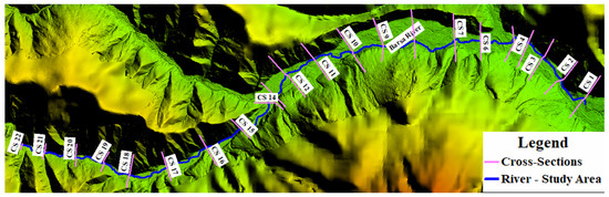
Figure 7.
Cross-sections for extracting results and training neural networks.
Although roughness and channel geometry are not direct inputs in the RNN models, they are inherently embedded in the training data, which are generated from HEC-RAS simulations that integrate Manning’s N coefficients and terrain-based hydrodynamic parameters. The networks thus learn from the effects these features produce on discharge and water level profiles.
The input data for the neural networks consist exclusively of the temporal evolution of discharge at the upstream section. Channel geometry and terrain roughness are not explicitly provided; however, their influence is already embedded in the training datasets extracted from the HEC-RAS model. As a result, the neural networks learn to anticipate the shapes of the flood wave and the water level downstream without direct access to the physical parameters of the catchment.
The input hydrographs were provided by INHGA within the Flood Risk Management Plan, while the water levels were automatically extracted from the results of 2D hydraulic simulations for the 22 control sections.
The third stage involves the construction of the neural networks [63]. The data obtained from the hydraulic modeling were edited and arranged in such a way that the networks could learn the variation patterns of discharge and water level both at each study section and along the river. Once the optimal data arrangement was determined, the training and testing of the neural networks commenced.
Figure 8 presents a simplified diagram of the neural architecture used for the five types of RNNs studied. Regarding the hidden layers, a technique based on three fully connected hidden layers was adopted. The number of neurons in these layers was carefully selected, drawing from the specialized literature [66], which recommends an architecture with a decreasing number of neurons from one layer to the next—an approach shown to offer clear advantages in analyzing problems involving temporal data sequences (such as hydrological data, temperature, or other time series).
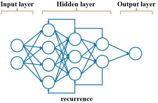
Figure 8.
Internal architecture of the recurrent neural networks studied.
For the first hidden layer, 256 neurons were chosen, a number considered suitable given the input data volume (approximately 31,000 elements). The second layer contains 128 neurons, reducing the size of the previous layer and serving to abstract the initial information, thereby helping to prevent overfitting. The final hidden layer further compacts the information with 64 neurons, supporting robust and more stable prediction.
After defining the internal architecture of the RNNs, the next step involved establishing how the data would be used. For training and testing purposes, the dataset was split into two subsets as follows: 80% of the data was used for training, while the remaining percentage was allocated for testing [67].
Another important parameter was the configuration of the time window over which the network would learn and retain data. The sequence length (i.e., the number of consecutive steps the model considers) was set to 10. This means the model always uses the previous 10 data points to predict the next one (the 11th). This value was chosen experimentally through a trial-and-error process and was found to yield the best results, providing the model with sufficient information about the temporal variation in discharge and water level, as well as the ability to detect trends in their changes.
Another essential parameter that needed to be defined is the activation function, which underpins the computations. In the present study, to maintain consistency across results and enable a clear comparison between the types of networks analyzed, the Rectified Linear Unit (ReLU) was chosen as the activation function. ReLU is one of the most widely used activation functions in deep learning, characterized by a simple and clear mathematical definition [68,69,70].
Thus, if the input value is positive, the function returns the value itself; if the input value is negative, the function returns 0. ReLU is a simple and fast function, with the major advantage of addressing the vanishing gradient problem, providing the model with greater stability and faster training.
The final parameter to be discussed in the RNN preparation phase is the algorithm used to adjust and optimize the neural weights. For this purpose, in order to improve prediction accuracy, the Adaptive Moment Estimation (ADAM) function was selected as the optimizer [71,72]. This is one of the most popular and high-performing optimization algorithms for most practical problems, with the capability to automatically adapt to each individual parameter, quickly adjusting the learning rate.
The fourth and final stage consists of generating new predictions using the trained RNNs. Starting with the information available for the seven AEP scenarios used in training the model, a new synthetic hydrograph was proposed, different in both maximum flow and flood wave volume. The hydrograph was created by interpolating between two known AEPs, 0.2% and 0.5%, respectively, using the passage coefficient, so it was easy to use this coefficient for both uniformly distributed flows between points and for the lateral inflows that the tributaries bring.
The new hydrograph was inserted at the upstream point of the model, considering the hypothesis of preserving the constant probability along the river and first propagated using the hydraulic modeling software HEC-Ras, following which the resulting flow and water level hydrographs were extracted in the 22 analyzed points. Moving towards the end of the workflow, the same newly created hydrograph was then propagated through each of the five RNN models studied.
After checking the training and testing metrics, we move on to the stage of extracting the results and validating them, and then towards the end of the experiment where a direct comparison of the obtained data is made. The next chapter synthesizes and analyzes the flow and water level hydrographs obtained at the key points of the models, comparing their peak values, presenting the results along the river, and evaluating the ability of the RNN models to predict the maximum flow, the free water level, the shape of the flood waves, and their volume.
3. Results and Discussion
The main objective of this study is to explore the ability of the RNN models used (S-RNN, LSTM, GRU, Bi-LSTM, and Bi-GRU) [73] in predicting and propagating a new synthetic flood wave along the river, this wave being constructed separately, different from the training data. The results obtained using the RNNs were then compared with the results obtained from classical modeling, concluding the capabilities of the approach.
For a clear and systematic analysis of the performance of the tested neural networks, the results were thematically grouped based on the type of metric used to evaluate the model’s prediction: prediction errors (MSE, RMSE), overall accuracy (NSE and ), volume errors, and the stability of the flood wave shape.
3.1. Evaluating Model Performance
3.1.1. Model Performance Metrics
Based on the formulas presented in Section 2.3 and given that in the S-RNN, LSTM, GRU, Bi-LSTM, and Bi-GRU models the performance indicators serve as a reliable benchmark for assessing result quality, this section reviews the most relevant values [74]. Metrics such as loss, NSE, MSE, RMSE, MAE, and provide insights into the accuracy, reliability, and overall effectiveness of the trained models in predicting time series data. The loss metric in this case uses the same formula as MSE, the fundamental difference between the two parameters as well as the values obtained, is that loss calculates the variations in errors during training, on a partial dataset, thus seeing the improvement of the model during training. In contrast, the final MSE is a global value, calculated only once on the entire dataset, reflecting the final accuracy of the model after the training process is complete.
The training and validation loss versus epoch graphs are shown in Table 3. Analyzing the images, it can be observed that the training and validation loss consistently decrease for all RNNs used, with the exception of LSTM and Bi-LSTM, which show slight oscillations between epoch 10 and epoch 20. However, in all cases, these values begin to stabilize after epoch 30.
Table 3.
Training and validations loss.
Regarding the final values of training and validation loss, they vary depending on the network used. For S-RNN, GRU, and Bi-GRU, the training loss is lower than the validation loss. In contrast, for LSTM and Bi-LSTM, the validation loss is slightly lower. These graphs are encouraging, indicating that the models learn effectively over the course of the 50 training epochs, even though some models reach convergence earlier.
Table 4 illustrate the evolution of the Nash–Sutcliffe Efficiency (NSE) coefficient as a function of the number of training epochs for each of the five RNN models studied. The graphs presented in this table reveal a general trend of rapid increase in NSE during the initial epochs, followed by stabilization near the value of 1, indicating strong performance in future predictions.
Table 4.
Nash–Sutcliffe efficiency model coefficient.
The bidirectional models (Bi-LSTM and Bi-GRU) appear to reach higher NSE values slightly earlier, suggesting more efficient learning of data dependencies.
The results presented in Table 5 provide a comparative summary of the evaluation metrics for the RNN models used, both for training and validation. The recorded values indicate good model training. The MSE and RMSE values show low errors, which is a sign of good generalization. Regarding the NSE and metrics, their values are very close to 1, suggesting that the models effectively reproduce the data used.
Table 5.
Model evaluation metrics.
The Bi-GRU model shows the lowest loss values for both training and validation, indicating strong performance. In contrast, the LSTM model displays higher values, suggesting a more difficult training process. Looking at the MSE and RMSE metrics, Bi-GRU again records the lowest values. Alongside Bi-GRU, the Bi-LSTM model also shows low values, indicating good generalization for both networks.
All models achieve very high NSE values, suggesting they effectively capture the dynamics of the data used. When examining MAE, Bi-LSTM and Bi-GRU also stand out with the lowest errors. Regarding the final metric, , values are very close to 1 across all models, but Bi-LSTM and Bi-GRU maintain slightly higher values in the validation phase, suggesting a slight edge in performance.
Overall, the bidirectional models demonstrate a modest but consistent superiority over the unidirectional ones across all metrics. NSE and are nearly perfect for all models, suggesting they are all capable of accurately replicating the hydrograph shape.
3.1.2. Prediction and Evaluation
After training the neural networks, the resulting model was saved separately to be used later for generating new predictions of discharge and water level hydrographs at the 22 analyzed sections.
The newly constructed hydrograph was propagated through both the 2D hydraulic model and the neural networks studied. The results obtained were extracted and compared both locally and globally, to determine the capacities of the networks.
The newly constructed hydrograph was first propagated in HEC-RAS, with results extracted at the 22 analysis sections and prepared for comparison with the predictions generated by the RNN models. To simplify the presentation process and highlight the key insights between the RNNs and classical modeling software, two analysis sections were selected for a detailed comparison. As shown in Figure 9, the two selected sections (highlighted in red) are section 13 and section 3. These were deliberately chosen due to their significant relevance within the model; section 13 is located downstream of the confluence between the Bârsa River and Bârsa lui Bucur River, while section 3 lies downstream of the confluence between the Bârsa River and Bârsa Fierului River.
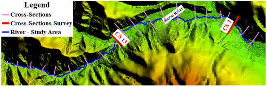
Figure 9.
Cross-sections for extracting results and training neural networks—two characteristic sections considered.
The following subchapters analyze the discharge and water level hydrographs at the two selected points, directly comparing the results in order to precisely assess the capabilities of the neural networks. This approach was chosen to highlight both the fundamental differences and the accuracy and predictive power of the RNNs in forecasting future events.
Results—Cross-Section 13
The first section analyzed is point 13 (CS 13), which is located at the first major discharge variation point along the Bârsa River, given its position downstream from the confluence with the Bârsa lui Bucur River. The tables below present the discharge (Table 6) and water level hydrographs (Table 7) extracted for each RNN model studied (predicted), followed by a comparison with the results from classical hydraulic modeling (observed). A summary table is also provided at the end, including the peak values and the resulting flood wave volume (Table 8).
Table 6.
RNN’s vs. HEC-Ras—cross-section 13—discharge.
Table 7.
RNN’s vs. HEC-Ras—cross-section 13—water surface elevation (WSE).
Table 8.
RNN’s vs. HEC-Ras—cross-section 13—summary table.
Analyzing the graphs and tables above, it can be observed that all studied RNNs demonstrate a strong ability to forecast and propagate a new hydrograph. When examining the discharge hydrograph plots, a close match between the observed and predicted data can be seen across all RNN models, indicating a high reconstruction capacity of the hydrographs.
In terms of quantitative results, all models exhibit discharge errors below 4%, well under the commonly accepted hydrological threshold of 10%. The lowest discharge errors are observed for GRU (0.8%), Bi-GRU (1.17%), and Bi-LSTM (1.33%), while the highest is recorded for LSTM at 3.61%.
Looking at the water level results given, the satisfactory discharge predictions are of good quality. The absolute differences between the reference values and the RNN-predicted values are small, ranging from −0.11 m for S-RNN to 0.05 m for Bi-GRU. S-RNN, LSTM, and GRU display slightly negative values (−0.11 m, −0.06 m, and −0.03 m), suggesting a mild underestimation of the peak level, while Bi-LSTM and Bi-GRU yield small positive deviations, indicating good alignment with the observed data.
Turning to the final variable compared to the flood wave volume four out of five RNNs show errors below 4%, with LSTM being the exception at 9.37%. The smallest errors are recorded for Bi-LSTM (2.43%) and Bi-GRU (2.74%). Based on these results, it can be concluded that the bidirectional networks deliver the best performance at this validation point, though all RNN models provide promising results.
Results—Cross-Sections 3
A similar analysis to that of the previous subchapter was conducted for section 3 (CS 3). The results obtained are discussed immediately following the figures.
Analyzing the results from section 3 (CS 3)—located downstream from the confluence between the Bârsa River and the Bârsa Fierului River, another area where discharge changes significantly (Table 9)—one can observe a good match between the observed values (from HEC-RAS) and those predicted by the RNNs when it comes to discharge. In this section as well, the bidirectional networks, especially Bi-GRU, show excellent alignment, particularly around the peak. On the other hand, the LSTM and GRU models display slight deviations from the hydrograph shape, especially during the rising limb of the flow.
Table 9.
RNN’s vs. HEC-Ras—cross-section 3—discharge.
Despite these differences, the highest discharge error between observed and predicted values is 4.15% for Bi-LSTM, while all other models remain under 3%. The S-RNN and LSTM networks tend to underestimate the discharge, producing lower predictions than the reference, whereas the GRU and bidirectional models tend to slightly overestimate the peak discharge.
As for water level results (Table 10), they show a good match between observed and predicted data, though all models exhibit slight offsets around the peak. The Bi-LSTM and Bi-GRU models are more consistent. In terms of absolute differences, the results in this section range from −0.05 m (S-RNN) to 0.04 m (Bi-GRU), indicating very small deviations.
Table 10.
RNN’s vs. HEC-Ras—cross-section 3—water surface elevation.
The relatively good match between the observed and simulated hydrographs leads to fairly accurate estimates of the flood wave volume in this section. LSTM is the only network to exhibit significant instability, with a volume error (Table 11) of 11.26%, mainly due to overestimation during the rising limb of the hydrograph. For the other models, the volume error remains around 3%, well below the acceptable threshold in hydrology.
Table 11.
RNN’s vs. HEC-Ras—cross-section 3—summary table.
Comparing the detailed results from the two analyzed sections—CS 3 and CS 13—slight differences can be observed. In CS 13, the bidirectional models and GRU provided the most accurate discharge estimates, while in CS 3, S-RNN and GRU performed best, and Bi-LSTM lost some accuracy. These aspects suggest that model performance appears to depend on the location of the section along the river. The water level results are good in both sections, with the largest deviation being −0.11 m for S-RNN in CS 13. CS 3 generally shows smaller, barely noticeable offsets. However, both Bi-GRU and Bi-LSTM tend to slightly overestimate hydrograph peaks in both cases.
Regarding the simulated flood wave volume, results indicate that the LSTM network performs the weakest in both sections, while the other four RNN models provide good performance.
Global Analysis Across the Entire Study Sector Regarding the Performance of the RNNs
The previous subchapters focused on a point-by-point analysis of the results in two key sections of the Bârsa River.
This last subchapter aims to analyze the results obtained starting from the same flood hydrograph along the entire length of the river [75], thus providing a much more detailed understanding of the outcomes and the capabilities that RNNs possess in predicting and propagating a new flood wave [76].
The longitudinal profile along the river shown in Figure 10 together with the details from Figure 11 and Figure 12 and the tabular results (Table 12) indicate satisfactory accuracy regarding the RNNs’ ability to propagate and predict a new water level. When examining the absolute difference between the reference level and the predicted level, the results show very small errors across the majority of the sections—for all models—ranging from −0.13 m (CS 15—S-RNN) to +0.06 m (CS 12—Bi-LSTM). The bidirectional models (Bi-LSTM, Bi-GRU) demonstrate the best spatial stability, consistently maintaining a nearly zero offset. In contrast, the LSTM network exhibited the most negative deviations (e.g., CS 2: −0.12 m), suggesting a slight underestimation of water levels.
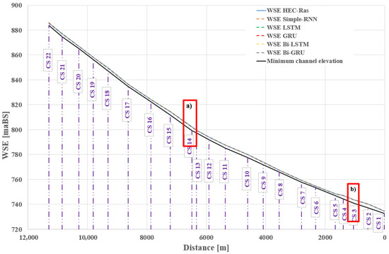
Figure 10.
Longitudinal profile along the Bârsa River.
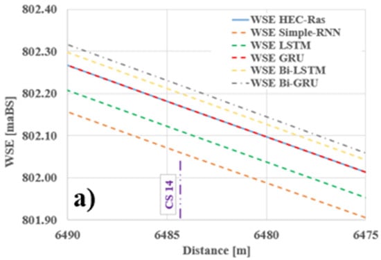
Figure 11.
Longitudinal profile along the Bârsa River—detail (a).
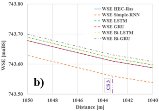
Figure 12.
Longitudinal profile along the Bârsa River—detail (b).
Table 12.
RNN’s vs. HEC-Ras—results table—water level.
The resulting peak discharges show locally variable errors, ranging from 0.01% to 7.43%, depending on the section and the model. GRU and Bi-GRU yield the lowest errors in most sections (Table 13). In contrast, LSTM displays significant errors in several sections reaching up to 7.43% in CS 20 and exceeding 6% in many other cases.
Table 13.
RNN’s vs. HEC-Ras—results table—maxim flow.
Flood wave volume proved to be a considerable challenge for LSTM, which recorded the highest deviations (between 6% and 11%) across most sections, with errors exceeding 9% in many instances (Table 14). The lowest errors were observed for GRU and S-RNN, particularly across all midstream sections (CS 10 to CS 1). Bi-GRU and Bi-LSTM networks remained consistent overall, although they occasionally exhibited a slight tendency to overestimate.
Table 14.
RNN’s vs. HEC-Ras—results table—flood wave volume.
The study results, summarized in Table 15, indicate that the GRU and Bi-GRU architectures delivered the best performance, with RMSE values below 1.63 and volume errors under 3% in over 80% of the analyzed sections. LSTM showed higher volume error values (sometimes exceeding 9%) in complex areas, suggesting relatively lower stability.
Table 15.
Summary table of results.
Average values for NSE and were close to 1 for all models, but GRU and Bi-GRU demonstrated the best consistency in preserving the hydrograph shape.
These results are consistent with the existing literature. For example, Zhang et al. (2023) [77] demonstrated the advantages of GRU architectures in both computational efficiency and predictive accuracy using lag-time preprocessing ( improved from 0.81 to 0.92 for STA-GRU) [78]. Studies conducted in Ellicott City confirmed the robustness of GRU over LSTM for hydrograph forecasting over 6–12 h, with values exceeding 0.9 [79]. The application of GRU for discharge and water level prediction in a mountainous basin showed superior performance compared to LSTM under various climatic and hydrological conditions [18,80].
In conclusion, this study provides empirical reinforcement for the use of GRU and Bi-GRU as efficient and stable alternatives to traditional hydraulic models in real-time flood warning applications.
3.2. Summary of Model Performance
For a synthetic understanding of the performance achieved by each neural model, the Table 16) presents the average values for the five main evaluation metrics.
Table 16.
Comparative table—Neural network performance.
The table above summarizes the performance of the five tested architectures in terms of absolute and relative errors for predicting water level, discharge, and flood volume. The GRU and Bi-GRU models clearly stand out with the best overall results. Although LSTM maintains high NSE and values, its increased volumetric error and deviation in hydrograph shapes suggest weaker performance under complex conditions.
These findings support the selection of GRU and Bi-GRU models for operational applications in flood forecasting.
4. Conclusions
The present study successfully demonstrates the potential of RNNs in predicting essential hydraulic characteristics, namely, peak discharge, water level, and flood wave volume within a new flood scenario on the Bârsa River. The methodological framework was robust, grounded in 2D hydraulic modeling using HEC-RAS and the analysis of five different recurrent neural network architectures (S-RNN, LSTM, GRU, Bi-LSTM, and Bi-GRU), evaluating their performance in simulating the propagation of a previously unknown flood wave.
This approach partially differs from the commonly known application of RNNs, as it fully emulates a 2D hydraulic model along the entire longitudinal profile of a river valley, based on synthetic hydrographs. This provides a fully reproducible and controlled testing framework.
When discussing overall model performance, all five RNN types yielded satisfactory results, with NSE and values extremely close to 1. This confirms the networks’ ability to learn from hydraulic data and their effectiveness in reproducing the shape of the flood wave. However, differences between architectures become more apparent in detailed prediction analysis such as wave shifting, peak overestimation, or errors in flood volume estimation.
The performance of the networks was clearly differentiated through quantitative analyses as follows: GRU achieved average RMSE values between 1.22 and 1.33 and MAE ≈ 0.27, while LSTM frequently exceeded 2.9 in RMSE and 10% in volume errors in downstream areas.
Across the entire assessment, GRU and Bi-GRU networks stood out for their balance between accuracy and stability. GRU achieved the lowest errors across all three key indicators (WSE, Q, Volume), followed closely by Bi-GRU, which showed a slight tendency to overestimate peak values. The Bi-LSTM and Bi-GRU networks performed particularly well in predicting water levels, giving them an advantage in that respect. Nevertheless, Bi-LSTM showed mild instabilities in peak discharge estimation in several sections, indicating higher local sensitivity. On the other hand, the LSTM network consistently performed the weakest, especially in estimating flood volume, with errors often exceeding 10% in multiple sections. Despite being a well-established architecture, LSTM showed lower adaptability in this study’s context.
The detailed evaluations in critical sections CS 13 (downstream of the confluence with Bârsa lui Bucur River) and CS 3 (downstream of the confluence with Bârsa Fierului River) enabled a fine-grained analysis. Here, good alignment was observed between the simulated hydrographs based on RNN and those obtained through classical modeling, particularly for the GRU, Bi-GRU, and S-RNN networks. Discharge and water level errors remained below 4%, while estimated volumes closely matched the reference values.
For the critical sections, the peak flow and flood volume values simulated by GRU and Bi-GRU remained within ±4% of the HEC-RAS model, validating their capability to accurately replicate the physical model.
The longitudinal profile highlighted the networks’ strong ability to generalize the flood wave prediction along the entire river segment. Absolute water level errors remained within ±0.1 m (with only a few isolated exceedances), demonstrating high confidence in their predictive capabilities.
These results indicate that the GRU and Bi-GRU networks not only have the potential to replace the execution of a full physical model, but they also provide a valid alternative for real-time applications, especially under hydrological emergency conditions.
This study’s approach indicates that the GRU network is highly recommended for future hydrological applications involving flood wave propagation, offering the best trade-off between simplicity and accuracy. The Bi-GRU model also delivered excellent results in this context, with the main trade-off being its increased complexity and longer training times.
The use of the GRU network is recommended for early warning systems, particularly in small or urban catchments where response time is limited and traditional simulations cannot be executed quickly.
For regional applications with complex hydrographic networks, Bi-GRU may offer a more accurate alternative, albeit with higher computational costs. Both models can be integrated into operational automatic forecasting workflows, eliminating the need to rerun mathematical models once the AI is trained.
Limitations and Future Direction
This study presents the analysis of synthetic hydrographs, having both the shape and the duration known, which makes them easier to understand by recurrent neural networks. Even if this is an advantage for the present work, at a global level it can be an important disadvantage. Thus, future research directions must consider irregular flood waves, having several peaks and different durations.
If we look at the results obtained, they clearly indicate that RNNs can be used for the propagation and forecasting of flood waves. Developing the algorithm by bringing in recorded data, enlarging the analyzed sector, either at the sub-basin or entire hydrographic basin level, as well as using more advanced network architectures, can be future research directions.
The working method can be transferred to specific areas, especially known to have a high risk of flooding, laying the foundation for a high-speed and high-performance flood warning system, based on artificial intelligence.
Funding
The elaboration of this methodology was not financed by public funds.
Data Availability Statement
The data owner is the S.C. AQUAPROJECT S.A., Romania (https://www.aquaproiect.ro/ accessed on 25 July 2025). Restrictions apply to the availability of these data according to the AQUAPROJECT policy.
Acknowledgments
The authors extend their gratitude to AQUAPROJECT for the availability and provision of all the materials needed to carry out the present study, as well as to the anonymous reviewers for their help and suggestions.
Conflicts of Interest
The authors declare no conflicts of interest.
References
- Tamm, O.; Saaremäe, E.; Rahkema, K.; Jaagus, J.; Tamm, T. The intensification of short-duration rainfall extremes due to climate change—Need for a frequent update of intensity–duration–frequency curves. Clim. Serv. 2023, 30, 100349. [Google Scholar] [CrossRef]
- Xu, Y.; Hu, T.; Chen, L.G.; Lu, H.; Chen, L.M.; Luna, Z.; Jin, Q.; Shi, Y. Impacts of Extreme Flood and Drought Events on Dish-Shaped Lake Habitats in Poyang Lake Under Altered Hydrological Regimes. Remote Sens. 2025, 17, 1936. [Google Scholar] [CrossRef]
- Gutierrez, L.L.; Huerta, A.; Llauca, H.; Bourrel, L.; Lavado-Casimiro, W. Assessment of Run-of-River and Hydropower Plants in Peru: Current and Potential Sites, Historical Variability (1981–2020), and Climate Change Projections (2035–2100). Climate 2025, 13, 125. [Google Scholar] [CrossRef]
- Spor, P.; Paşa, Y.; Doğan, E. Evaluation of Simulation Results of HEC-RAS Coupled 1D/2D and 2D Modeling Approaches Through Scenario-Based Analysis. Water 2025, 17, 1163. [Google Scholar] [CrossRef]
- Zhao, M.; Li, Y.; Li, L.; Dai, W. Response of Riverbed Shaping to a Flood Event in the Reach from Alar to Xinquman in the Mainstream of the Tarim River. Water 2025, 17, 1092. [Google Scholar] [CrossRef]
- Oliva, A.; Olcina, J. Floods and Structural Anthropogenic Barriers (Roads and Waterworks) Affecting the Natural Flow of Waters: Hydraulic Modelling and Proposals for the Final Section of the River Segura (Spain). GeoHazards 2024, 5, 1220–1246. [Google Scholar] [CrossRef]
- Becke, A.S. Evolution of deep learning trends between 2012 and 2020: A perspective from the EJR editorial board. Eur. J. Radiol. 2022, 155, 110462. [Google Scholar] [CrossRef]
- Waqas, M.; Humphries, U.W. A critical review of RNN and LSTM variants in hydrological time series predictions. MethodsX 2025, 13, 102946. [Google Scholar] [CrossRef]
- Tripathy, K.P.; Mishra, A.K. Deep learning in hydrology and water resources disciplines: Concepts, methods, applications, and research directions. J. Hydrol. 2024, 628, 130458. [Google Scholar] [CrossRef]
- Mtsweni, S.; Bakare, B.F.; Rathilal, S. Artificial Neural Network-Based Prediction of Clogging Duration to Support Backwashing Requirement in a Horizontal Roughing Filter: Enhancing Maintenance Efficiency. Water 2025, 17, 2319. [Google Scholar] [CrossRef]
- Luo, J.; Zhu, D.; Li, D. Classification-enhanced LSTM model for predicting river water levels. J. Hydrol. 2025, 650, 132535. [Google Scholar] [CrossRef]
- Dabire, N.; Ezin, E.C.; Firmin, A.M. Forecasting Lake Nokoué Water Levels Using Long Short-Term Memory Network. Hydrology 2024, 11, 161. [Google Scholar] [CrossRef]
- Nguyen, A.D.; Vu, V.H.; Hoang, D.V.; Nguyen, T.D.; Nguyen, K.; Le Nguyen, P.; Ji, Y. Attentional ensemble model for accurate discharge and water level prediction with training data enhancement. Eng. Appl. Artif. Intell. 2023, 126, 107073. [Google Scholar] [CrossRef]
- Heidari, E.; Samadi, V.; Khan, A.A. Leveraging Recurrent Neural Networks for Flood Prediction and Assessment. Hydrology 2025, 14, 90. [Google Scholar] [CrossRef]
- Gholizadeh, H.; Zhang, Y.; Frame, J.; Gu, X.; Green, C.T. Long short-term memory models to quantify long-term evolution of streamflow discharge and groundwater depth in Alabama. Sci. Total Environ. 2023, 901, 165884. [Google Scholar] [CrossRef]
- Naghashi, V.; Boukadoum, M.; Diallo, A.B. Should We Reconsider RNNs for Time-Series Forecasting? AI 2025, 6, 90. [Google Scholar] [CrossRef]
- Li, G.; Zhu, H.; Jian, H.; Zha, W.; Wang, J.; Shu, Z.; Yao, S.; Han, H. A combined hydrodynamic model and deep learning method to predict water level in ungauged rivers. J. Hydrol. 2023, 625, 130025. [Google Scholar] [CrossRef]
- Rugină, A.M. The Use of Recurrent Neural Networks (S-RNN, LSTM, GRU) for Flood Forecasting Based on Data Extracted from Classical Hydraulic Modeling. Model. Civ. Environ. Eng. 2023, 18, 1–18. [Google Scholar] [CrossRef]
- Li, J.; Zhang, X.; Yu, R.; Zhang, L.; Wu, J. Deep learning combined with attention mechanism for multi-time-step runnof prediction modelig. Univ. Politeh. Buchar. Sci. Bull. Ser. C Electical Eng. Comput. Sci. 2025, 87, 2. [Google Scholar]
- ANAR; INGHA. Flood Risk Management Plan—Olt Water Basin Administration. In RO: Planul de Management al Riscului la Inundații; Administrația Bazinală de Apă Olt: Râmnicu Vâlcea, Romania, 2015; Available online: https://olt.rowater.ro/abaolt/wp-content/uploads/2021/03/6-PMRI-Olt.pdf (accessed on 12 May 2025).
- Hidri, A.; Alsaif, S.A.; Alahmari, M.; AlShehri, E.; Hidri, M.S. Opinion Mining and Analysis Using Hybrid Deep Neural Networks. Technologies 2025, 13, 175. [Google Scholar] [CrossRef]
- Akkala, A.; Boubrahimi, S.F.; Hamdi, S.M.; Hosseinzadeh, P.; Nassar, A. Spatio-Temporal Graph Neural Networks for Streamflow Prediction in the Upper Colorado Basin. Hydrology 2025, 12, 60. [Google Scholar] [CrossRef]
- Workneh, H.A.; Jha, M.K. Utilizing Deep Learning Models to Predict Streamflow. Water 2025, 17, 756. [Google Scholar] [CrossRef]
- Aksoy, B. Flood Analysis in Lower Filyos Basin Using HEC-RAS and HEC-HMS Software. Sustainability 2025, 17, 5220. [Google Scholar] [CrossRef]
- Kausik, A.K.; Rashid, A.B.; Baki, R.F.; Maktum, M.M.J. Machine learning algorithms for manufacturing quality assurance: A systematic review of performance metrics and applications. Array 2025, 26, 100393. [Google Scholar] [CrossRef]
- Wang, D.; Li, Q.; Liu, S.; Li, P.; Li, J. Long-term river flow forecasting: An integrated deep learning model with multi-scale feature extraction. Expert Syst. Appl. 2025, 281, 127387. [Google Scholar] [CrossRef]
- Situ, Z.; Zhong, Q.; Zhang, J.; Teng, S.; Ge, X.; Zhou, Q.; Zhao, Z. Attention-based deep learning framework for urban flood damage and risk assessment with improved flood prediction and land use segmentation. Int. J. Disaster Risk Reduct. 2025, 116, 105165. [Google Scholar] [CrossRef]
- Lee, J.H.; Yuk, G.M.; Moon, H.T.; Moon, Y. Integrated Flood Forecasting and Warning System against Flash Rainfall in the Small-Scaled Urban Stream. Atmosphere 2020, 11, 971. [Google Scholar] [CrossRef]
- ANAR; INGHA. Flood Risk Management Plan—Olt Water Basin Administration—Cycle II of implementation of the Floods Directive 2007/60/EC. In RO: Planul de Management al Riscului la Inundații—Ciclul II De implementare a Directivei Inundaţii 2007/60/CE; Administrația Bazinală de Apă Olt: Râmnicu Vâlcea, Romania, 2023; Available online: https://inundatii.ro/wp-content/uploads/2023/09/PMRI_Ciclul-II_ABA-Olt.pdf (accessed on 3 June 2025).
- Li, X.; Lin, J.; Zhao, W.; Wen, F. Approximate calculation of flash flood maximum inundation extent in small catchment with large elevation difference. J. Hydrol. 2020, 590, 125195. [Google Scholar] [CrossRef]
- El-Hames, A.S. An empirical method for peak discharge prediction in ungauged arid and semi-arid region catchments based on morphological parameters and SCS curve number. J. Hydrol. 2012, 456–457, 94–100. [Google Scholar] [CrossRef]
- RO-FLOODS. 2023. Available online: https://inundatii.ro/ro-floods/ (accessed on 14 May 2025).
- Rahman, M.; Ali, S. Drivers of tidal flow variability in the Pussur fluvial estuary: A numerical study by HEC-RAS. Heliyon 2024, 10, e25662. [Google Scholar] [CrossRef]
- Schäppi, B.; Perona, P.; Schneider, P.; Burlando, P. Integrating river cross section measurements with digital terrain models for improved flow modelling applications. Comput. Geosci. 2012, 36, 707–716. [Google Scholar] [CrossRef]
- Rezende, I.; Fatras, C.; Oubanas, H.; Gejadze, I.; Malaterre, P.-O.; Peña-Luque, S.; Domeneghetti, A. Reconstruction of Effective Cross-Sections from DEMs and Water Surface Elevation. Remote Sens. 2025, 17, 1020. [Google Scholar] [CrossRef]
- Chow, V.T. Open-Channel Hydraulics; International Student Edition; McGraw-Hill Book Company, Inc.: New York, NY, USA; Kogakusha Company, Ltd.: Tokyo, Japan, 1959. [Google Scholar]
- Copernicus. Land Monitoring Service. Available online: https://land.copernicus.eu/en/products/corine-land-cover (accessed on 5 March 2025).
- Ovadia, O.; Kahana, A.; Turkel, E.; Dekel, S. Beyond the Courant-Friedrichs-Lewy condition: Numerical methods for the wave problem using deep learning. J. Comput. Phys. 2021, 442, 110493. [Google Scholar] [CrossRef]
- Zhou, H.; Liu, Y.; Wang, J. Acoustic finite-difference modeling beyond conventional Courant-Friedrichs-Lewy stability limit: Approach based on variable-length temporal and spatial operators. Earthq. Sci. 2021, 34, 123–136. [Google Scholar] [CrossRef]
- Wichitrnithed, C.; Valseth, E.; Kubatko, E.J.; Kang, Y.; Hudson, M.; Dawson, C. A discontinuous Galerkin finite element model for compound flood simulations. Comput. Methods Appl. Mech. Eng. 2024, 420, 116707. [Google Scholar] [CrossRef]
- Köksoy, O. Multiresponse robust design: Mean square error (MSE) criterion. Appl. Math. Comput. 2006, 175, 1716–1729. [Google Scholar] [CrossRef]
- Karunasingha, D.S.K. Root mean square error or mean absolute error? Use their ratio as well. Inf. Sci. 2022, 585, 609–629. [Google Scholar] [CrossRef]
- Myttenaere, A.; Golden, B.; Grand, B.; Rossi, F. Mean Absolute Percentage Error for regression models. Neurocomputing 2016, 192, 38–48. [Google Scholar] [CrossRef]
- Tang, H.; Mayersohn, M. Utility of the Coefficient of Determination (R2) in Assessing the Accuracy of Interspecies Allometric Predictions: Illumination or Illusion? Drug Metab. Dispos. 2007, 35, 2139–2142. [Google Scholar] [CrossRef]
- Timilsina, S.; Passalacqua, P. A comparative analysis of national water model versions 2.1 and 3.0 reveals advances and challenges in streamflow predictions during storm events. J. Hydrol. Reg. Stud. 2025, 58, 102196. [Google Scholar] [CrossRef]
- Althoff, D.; Rodrigues, L.N. Goodness-of-fit criteria for hydrological models: Model calibration and performance assessment. J. Hydrol. 2021, 600, 126674. [Google Scholar] [CrossRef]
- Alkaabi, K.; Sarfraz, U.; Darmaki, S.A. A Deep Learning Framework for Flash-Flood-Runoff Prediction: Integrating CNN-RNN with Neural Ordinary Differential Equations (ODEs). Water 2025, 17, 1283. [Google Scholar] [CrossRef]
- Koutsoyiannis, D. When Are Models Useful? Revisiting the Quantification of Reality Checks. Water 2025, 17, 264. [Google Scholar] [CrossRef]
- Zhao, X.; Wang, H.; Bai, M.; Xu, Y.; Dong, S.; Rao, H.; Ming, W. A Comprehensive Review of Methods for Hydrological Forecasting Based on Deep Learning. Water 2024, 16, 1407. [Google Scholar] [CrossRef]
- Tina, Y.; Xu, Y.-P.; Yang, Z.; Wang, G.; Zhu, Q. Integration of a Parsimonious Hydrological Model with Recurrent Neural Networks for Improved Streamflow Forecasting. Water 2018, 10, 1655. [Google Scholar] [CrossRef]
- Kang, J.; Wang, H.; Yuan, F.; Wang, Z.; Huang, J.; Qiu, T. Prediction of Precipitation Based on Recurrent Neural Networks in Jingdezhen, Jiangxi Province, China. Atmosphere 2020, 11, 246. [Google Scholar] [CrossRef]
- Ubal, C.; Di-Giorgi, G.; Contreras-Reyes, J.E.; Salas, R. Predicting the Long-Term Dependencies in Time Series Using Recurrent Artificial Neural Networks. Mach. Learn. Knowl. Extr. 2023, 5, 1340–1358. [Google Scholar] [CrossRef]
- Hochreiter, S.; Schmidhuber, J. Long Short-Term Memory. Neural Comput. 1997, 9, 1735–1780. [Google Scholar] [CrossRef]
- Fan, H.; Jiang, M.; Xu, L.; Zhu, H.; Cheng, J.; Jiang, J. Comparison of Long Short Term Memory Networks and the Hydrological Model in Runoff Simulation. Water 2020, 12, 175. [Google Scholar] [CrossRef]
- Cho, K.; Kim, Y. Improving streamflow prediction in the WRF-Hydro model with LSTM networks. J. Hydrol. 2022, 605, 127297. [Google Scholar] [CrossRef]
- Nifa, K.; Boudhar, A.; Ouatiki, H.; Elyoussfi, H.; Bargam, B.; Chehbouni, A. Deep Learning Approach with LSTM for Daily Streamflow Prediction in a Semi-Arid Area: A Case Study of Oum Er-Rbia River Basin, Morocco. Water 2023, 15, 262. [Google Scholar] [CrossRef]
- Seifi, A.; Pourebrahim, S.; Ehteram, M.; Shabanian, H. A robust multi-model framework for groundwater level prediction: The BFSA-MVMD-GRU-RVM model. Results Eng. 2024, 24, 103250. [Google Scholar] [CrossRef]
- Gharehbaghi, A.; Ghasemlounia, R.; Ahmadi, F.; Albaji, M. Groundwater level prediction with meteorologically sensitive Gated Recurrent Unit (GRU) neural networks. J. Hydrol. 2022, 612, 128262. [Google Scholar] [CrossRef]
- Jamei, M.; Ali, M.; Malik, A.; Karbasi, M.; Rai, P.; Yaseen, Z.M. Development of a TVF-EMD-based multi-decomposition technique integrated with Encoder-Decoder-Bidirectional-LSTM for monthly rainfall forecasting. J. Hydrol. 2023, 617, 129105. [Google Scholar] [CrossRef]
- Jin, L.; Xue, H.; Dong, G.; Han, Y.; Li, Z.; Lian, Y. Coupling the remote sensing data-enhanced SWAT model with the bidirectional long short-term memory model to improve daily streamflow simulation. J. Hydrol. 2024, 634, 131117. [Google Scholar] [CrossRef]
- Chen, C.; Jiang, J.; Zhou, Y.; Lv, N.; Liang, X.; Wan, S. An edge intelligence empowered flooding process prediction using Internet of things in smart city. J. Parallel Distrib. Comput. 2022, 165, 66–78. [Google Scholar] [CrossRef]
- Jamei, M.; Ali, M.; Karbasi, M.; Sharma, E.; Jamei, M.; Chu, X.; Yaseen, Z.M. A high dimensional features-based cascaded forward neural network coupled with MVMD and Boruta-GBDT for multi-step ahead forecasting of surface soil moisture. Eng. Appl. Artif. Intell. 2023, 120, 105895. [Google Scholar] [CrossRef]
- Feng, Z.K.; Zhang, J.S.; Niu, W.J. A state-of-the-art review of long short-term memory models with applications in hydrology and water resources. Appl. Soft Comput. 2024, 167, 112352. [Google Scholar] [CrossRef]
- Sim, Y.; Shin, W.; Lee, S. Automated code transformation for distributed training of TensorFlow deep learning models. Sci. Comput. Program. 2025, 242, 103260. [Google Scholar] [CrossRef]
- Parisi, L.; Ma, R.; Chandran, N.R.; Lanzillotta, M. hyper-sinh: An accurate and reliable function from shallow to deep learning in TensorFlow and Keras. Mach. Learn. Appl. 2021, 6, 100112. [Google Scholar] [CrossRef]
- Casolaro, A.; Capone, V.; Iannuzzo, G.; Camastra, F. Deep Learning for Time Series Forecasting: Advances and Open Problems. Information 2023, 14, 598. [Google Scholar] [CrossRef]
- Wei, X.; Zhang, L.; Yang, H.-Q.; Zhang, L.; Yao, Y.-P. Machine learning for pore-water pressure time-series prediction: Application of recurrent neural networks. Geosci. Front. 2021, 12, 453–467. [Google Scholar] [CrossRef]
- Hosseini, A.; Guay, M.; Li, X. On ReLU neural networks as piecewise linear surrogate models. Comput. Chem. Eng. 2025, 201, 109208. [Google Scholar] [CrossRef]
- Cabanilla, K.I.M.; Mohammad, R.Z.; Lope, J.E.C. Neural networks with ReLU powers need less depth. Neural Netw. 2024, 172, 106073. [Google Scholar] [CrossRef] [PubMed]
- Xu, Y.; Zhang, H. Convergence of deep ReLU networks. Neurocomputing 2024, 571, 127174. [Google Scholar] [CrossRef]
- Aula, S.A.; Rashid, T.A. Foxtsage vs. Adam: Revolution or evolution in optimization? Cogn. Syst. Res. 2025, 92, 101373. [Google Scholar] [CrossRef]
- Le-Duc, T.; Nguyen-Xuan, H.; Lee, J. Sequential motion optimization with short-term adaptive moment estimation for deep learning problems. Eng. Appl. Artif. Intell. 2024, 129, 107593. [Google Scholar] [CrossRef]
- Gao, S.; Huang, Y.; Zhang, S.; Han, J.; Wang, G.; Zhang, M.; Lin, Q. Short-term runoff prediction with GRU and LSTM networks without requiring time step optimization during sample generation. J. Hydrol. 2020, 589, 125188. [Google Scholar] [CrossRef]
- Liu, P.; Wang, L.; Ranjan, R.; He, G.; Zhao, L. A Survey on Active Deep Learning: From Model Driven to Data Driven. ACM Comput. Surv. (CSUR) 2022, 54, 221. [Google Scholar] [CrossRef]
- Sun, A.Y.; Jiang, P.; Yang, Z.-L.; Xie, Y.; Chen, X. A graph neural network (GNN) approach to basin-scale river network learning: The role of physics-based connectivity and data fusion. Hydrol. Earth Syst. Sci. 2022, 26, 5163–5184. [Google Scholar] [CrossRef]
- Rahimzad, M.; Nia, A.M.; Zolfonoon, H.; Soltani, J.; Mehr, A.D.; Kwon, H.-H. Performance Comparison of an LSTM-based Deep Learning Model versus Conventional Machine Learning Algorithms for Streamflow Forecasting. Water Resour. Manag. 2021, 35, 4167–4187. [Google Scholar] [CrossRef]
- Zhang, Y.; Zhou, Z.; Thé, J.V.G.; Yang, S.X.; Gharabaghi, B. Flood Forecasting Using Hybrid LSTM and GRU Models with Lag Time Preprocessing. Water 2023, 15, 3982. [Google Scholar] [CrossRef]
- Fordjour, G.; Kalyanapu, A.J. Implementing a GRU neural network for flood prediction in Ashland City, Tennessee. Cornell Univ. Comput. Sci. Mach. Learn. 2024, arXiv:2405.10375. [Google Scholar] [CrossRef]
- Oddo, P.C.; Bolten, J.D.; Kumar, S.V.; Cleary, B. Deep Convolutional LSTM for improved flash flood prediction. Front. Water 2024, 6, 1346104. [Google Scholar] [CrossRef]
- Widiasari, I.R.; Efendi, R. Utilizing LSTM-GRU for IOT-Based Water Level Prediction Using Multi-Variable Rainfall Time Series Data. Informatics 2024, 11, 73. [Google Scholar] [CrossRef]


Disclaimer/Publisher’s Note: The statements, opinions and data contained in all publications are solely those of the individual author(s) and contributor(s) and not of MDPI and/or the editor(s). MDPI and/or the editor(s) disclaim responsibility for any injury to people or property resulting from any ideas, methods, instructions or products referred to in the content. |
© 2025 by the author. Licensee MDPI, Basel, Switzerland. This article is an open access article distributed under the terms and conditions of the Creative Commons Attribution (CC BY) license (https://creativecommons.org/licenses/by/4.0/).