Addressing Volatility and Nonlinearity in Discharge Modeling: ARIMA-iGARCH for Short-Term Hydrological Time Series Simulation

Abstract

Selecting an appropriate model for discharge simulation remains a fundamental challenge in modeling. While artificial neural networks (ANNs) have been widely accepted due to detecting streamflow patterns, they require large datasets for efficient training. However, when short-term datasets are available, training ANNs becomes problematic. Autoregressive integrated moving average (ARIMA) models offer a promising alternative; however, severe volatility, nonlinearity, and trends in hydrological time series can still lead to significant errors. To address these challenges, this study introduces a new adaptive hybrid model, ARIMA-iGARCH, designed to account volatility, variance inconsistency, and nonlinear behavior in short-term hydrological datasets. We apply the model to four hourly discharge time series from the Schwarzbach River at the Nauheim gauge in Hesse, Germany, under the assumption of normally distributed residuals. The results demonstrate that the specialized parameter estimation method achieves lower complexity and higher accuracy. For the four events analyzed, R² values reached 0.99, 0.96, 0.99, and 0.98; RMSE values were 0.031, 0.091, 0.023, and 0.052. By delivering accurate short-term discharge predictions, the ARIMA-iGARCH model provides a basis for enhancing water resource planning and flood risk management. Overall, the model significantly improves modeling long memory, nonlinear, nonstationary shifts in short-term hydrological datasets by effectively capturing fluctuations in variance.

1. Introduction

A flood is one of the most prevalent hydrological phenomena. Due to its suddenness, it can profoundly influence water resources, ecology, and human activities, posing significant challenges for water management and infrastructure resilience. Accordingly, modeling of streamflow, as a crucial component of hydrological cycle, can be considered the most important factor for managing flood. Therefore, it is important to accurately model streamflow behavior in order to predict natural disasters with the aim of mitigating the risks of their impacts [1,2,3]. The complex relationships between atmosphere, terrestrial, and water cycle can be recognized by hydrological models, and in fact, these models are the effective streamflow prediction tools [4,5,6,7]. In general, there are two categories of the hydrological models: physically based and mathematically based [8,9]. Physically based models perform modeling by considering hydro-meteorological variables that have an effect on hydrological phenomena. On the other hand, mathematically based models perform modeling by using previous correlation between the historical data and the relationships between target and independent variables. Moreover, easy implementation, low input requirements, minimal effort for development, and moderate computational resources are the advantages offered by mathematically based models [10]. Due to their high ability in nonlinear modeling, there has been an extensively growing interest in the application of data-driven techniques such as machine learning (ML), including artificial neural networks (ANNs), genetic programming (GP), adaptive neuro-fuzzy inference systems (ANFISs), and wavelet transform (WT), in hydrological time series prediction [11,12,13,14,15]. Despite the considerable capabilities inherent in ML methods, particularly deep learning models, still, challenges persist with this type of method:

• One of the major challenges researchers are faced with is that ML methods are data-hungry and need long-term and extensive amounts of data for training [16,17]. However, sometimes only short-term datasets are available.
• In addition, the dependence of ML algorithm effectiveness on input-data representation integrity can pose another challenge. Constructing features from raw data is a significant part of the modeling, and this is extremely field-specific, requiring substantial human effort [18].
• Furthermore, ML techniques are examined with the intention of functioning as a black box. This issue is common in fields such as bioinformatics [19], but in fields such as medicine and disease diagnosis, not only the result but also the method of obtaining the result is important [20].
• Additionally, the need to continually train and adapt to new information without forgetting or degrading performance on previously trained tasks can pose another critical challenge, crucial for such applications like biology [21,22].
• On the other hand, overfitting is one of the known problems that researchers are dealing with. Overfitting significantly affects model performance [23,24,25].
• Moreover, the vanishing gradient problem is another issue that can cause a reduction in efficient model performance. This problem can appear while using backpropagation and gradient-based learning techniques, usually in the training step [26,27,28,29].

In response to these challenges, turning to hybrid models that combine the strengths of different methodologies to overcome their individual limitations can be an effective strategy. In recent decades, linear time series models have been widely applied in hydrology fields such as flood analysis [10,30,31,32], rainfall [33,34,35,36], streamflow [37,38,39,40,41], and droughts [42,43,44]. ARIMA generally models the mean behavior of the time series. Its efficacy in modeling has been affirmed in recent research studies [45,46,47,48]. However, ARIMA assumes that the residual series has a normal independent linear distribution and does not capture nonlinear patterns [11,49]. Therefore, due to the variation in residuals changing over time, ARIMA is insufficient for streamflow modeling. Recently, an upward trend can be observed in the utilization of combinations of nonlinear models with ARIMA, with the aim of capturing volatility in hydrology. However, GARCH is commonly used for modeling the variance of time series [50,51], and connecting the GARCH model with the single-mean ARIMA improves the model performance regarding volatility [52,53]. ARIMA-iGARCH considers both short-term fluctuations and long-term trends [54]. Time-varying variance or volatility, known as autoregressive conditional heteroscedasticity, is a characteristic of a time series affected by an ARCH or GARCH effect. This phenomenon represents the second-order moment of the residual time series. In this behavior, large changes typically follow previous large changes, while small changes tend to follow small changes [29]. This manner, termed conditional heteroscedasticity, can be effectively modeled using ARCH-type models due to its autoregressive structure. ARCH and GARCH methods are the common types of these models, and they remove the ARCH effect. Mo et al. [30] developed both LSTM and GARCH approaches for long-term deterministic streamflow forecasts and statistical evaluation of time-varying errors, producing a probabilistic forecast that accounts for uncertainty. The findings show GARCH’s strong capability to capture time-varying forecast errors, reducing forecast failure probability and enhancing probabilistic forecast accuracy. Sarhadi et al. [53] accurately identified the short memory in drought compounds using bivariate dynamic GARCH, revealing a strong relationship between hydrological and meteorological droughts. Kandukuri [55] recommend hybrid models, such as ARIMA-GARCH, over empirical models for capturing daily time series volatility, noting their effectiveness in short-interval dynamics. While GARCH models offer insights into time-varying volatility, challenges remain, particularly in capturing long memory effects and volatility asymmetries, as well as accounting for volatility persistence and structural breaks in time series [56,57,58]. These limitations can compromise the accuracy and reliability of modeling.

To address these shortcomings, integrated GARCH (iGARCH) has the potential to be the optimal solution and offers a novel approach to address volatility and dynamic variance in hydrological data. As far as the authors are aware, modeling the short-term discharge time series by developing the hybrid model iGARCH-ARIMA has not yet been explored. Specifically, the objectives of this study are 1. to develop an ARIMA-iGARCH hybrid model that integrates an autoregressive integrated moving average (ARIMA) model and an integrated generalized autoregressive conditional heteroscedasticity (iGARCH) model; 2. to apply the newly developed, innovative hybrid model to selected datasets; 3. to investigate the model performance when modeling the hourly streamflow short-term time series; and 4. to assess whether the combination of the time series modeling capabilities of ARIMA and the volatility modeling prowess of iGARCH provides benefits. The proposed ARIMA-iGARCH model demonstrates superior performance in capturing both the mean dynamics and volatility clustering of short-term discharge series, offering a promising tool for infrastructure protection, emergency planning, and community resilience. The ARIMA-iGARCH model integrates linear and volatility modeling techniques to bridge the gap left by data-intensive deep learning methods, offering a robust solution for short-term hydrological forecasting when limited data is available. While ARIMA is proficient at modeling linear dependencies and capturing the mean structure of discharge series, it assumes constant variance, which is often violated in natural systems influenced by external shocks and seasonal extremes. The iGARCH component addresses this shortcoming by capturing persistent conditional heteroscedasticity, common in hydrological data, where the impact of shocks decays slowly over time. This makes the introduced ARIMA-iGARCH framework particularly suitable for modeling the complex dynamics inherent in hydrological time series, especially for short-term data. Its capacity to simultaneously model both the evolving mean and variance processes enhances predictive reliability, which is especially critical in flood-early-warning and water-resource-management applications. In contrast to models like standalone ARIMA, LSTM, or traditional GARCH variants, ARIMA-iGARCH offers a transparent and interpretable structure with improved responsiveness to changes in variance patterns. This combination enhances both prediction accuracy and the ability to capture evolving volatility in hydrological time series.

This paper is organized as follows: Section 2 provides the case study and data collection, methodology is described in Section 3, results and discussion are illustrated in Section 4, finally Section 5 presents the conclusion.

2. Case Study and Data Collection

To develop and test different statistical and AI methods for adequate flood prediction, a study area was selected, which is also test area of the LOEWE Research Centre ‘emergenCITY’ (https://www.emergencity.de (accessed on 5 June 2023)). The main aim of the project is to protect smart cities from disasters by developing resilient infrastructures that save human lives. Our analyses were part of the sub-project ‘Smart flood and low flow warning system’ with the objective to develop an environmental monitoring and warning system for early assessment and warning of flooding and low flows based on real-time measurement data with data fusion from various sources using artificial intelligence. Within this project, we gained several information from the catchment of the Schwarzbach river upstream of the gauge Nauheim (ID 23980353; coordinates 49.9508, 8.4526; [59]). The gauge is located in the federal state of Hesse in Germany in the district of Groß-Gerau. The catchment size is 135 km² [59] and is part of the Rhine River Basin district. The catchment is characterized by a flat landscape, belonging to the Rhine River Plain. Land use is mainly rural, but there are a few larger settlements, such as the towns of Mörfelden-Walldorf and Langen, and the municipality of Nauheim. Additionally, Frankfurt Airport, the largest airport of Germany, is located in the northern part of the catchment area. Figure 1 shows the catchment and the exact location of the gauge Nauheim. The yellow-shaded area indicates the Schwarzbach catchment. The Schwarzbach stream originates from the confluence of the streams Gundbach and Geräthsbach, flows in a south-westerly direction, and first forms the northern settlement boundary of Nauheim and then flows through the middle of Nauheim, where the Nauheim gauge is located. Main discharge values (period 1965–2009) for the gauging station are as follows: mean discharge MQ is 0.60 m³/s with lowest discharge value NQ 0.02 m³/s (28 August 1976) and highest discharge value HQ 5.00 m³/s (11 June 1965) [60].

For this study, four flood events were picked (

Table 1. Four selected flood events (data source: HLNUG 2023a [16]) and heavy rainfall events (data source: DWD 2023 [61], Frankfurt airport weather station).

Event	Period	N(Q) *	Max. Q [m3/s (Date and Time)]	N(P) **	Max. Precipitation Intensity [mm/h (Date and Time)]
1	8–14 June 2013	577	1.83 (at 9 June 2013 16:15–18:00)	865	34.8 (8 June 2013 18:00)
2	15–20 August 2012	481	1.78 (at 16 August 2012 11:45–14:45)	721	37.3 (16 August 2012 02:00)
3	20–26 July 2004	577	1.18 (at 24 July 2004 04:45–11:45)	865	37.4 (23 July 2004 19:00)
4	1–7 May 2000	577	1.80 (at 2 May 2000 16:15–16:30)	865	25.9 (4 May 2000 00:00)

* Note: N(Q) is number of discharge data (15 minutes’ resolution). ** Note: N(P) is number of precipitation data (10 minutes’ resolution).

). The events were selected in such a way that they could be related to heavy rainfall events (>25 mm/h) in spring/summer and could be defined as individual events. The discharge data was available in 15 min steps (1985–2023, data source: [16]). The precipitation data was measured at Frankfurt Airport in 10 min resolution for 1993–2023 (DWD Station Frankfurt/M. (Flughfn.) ID 1420, [61]).

Figure 1. Schwarzbach catchment upstream of Nauheim gauge (after HLNUG 2022 [62]).

Figure 1. Schwarzbach catchment upstream of Nauheim gauge (after HLNUG 2022 [62]).

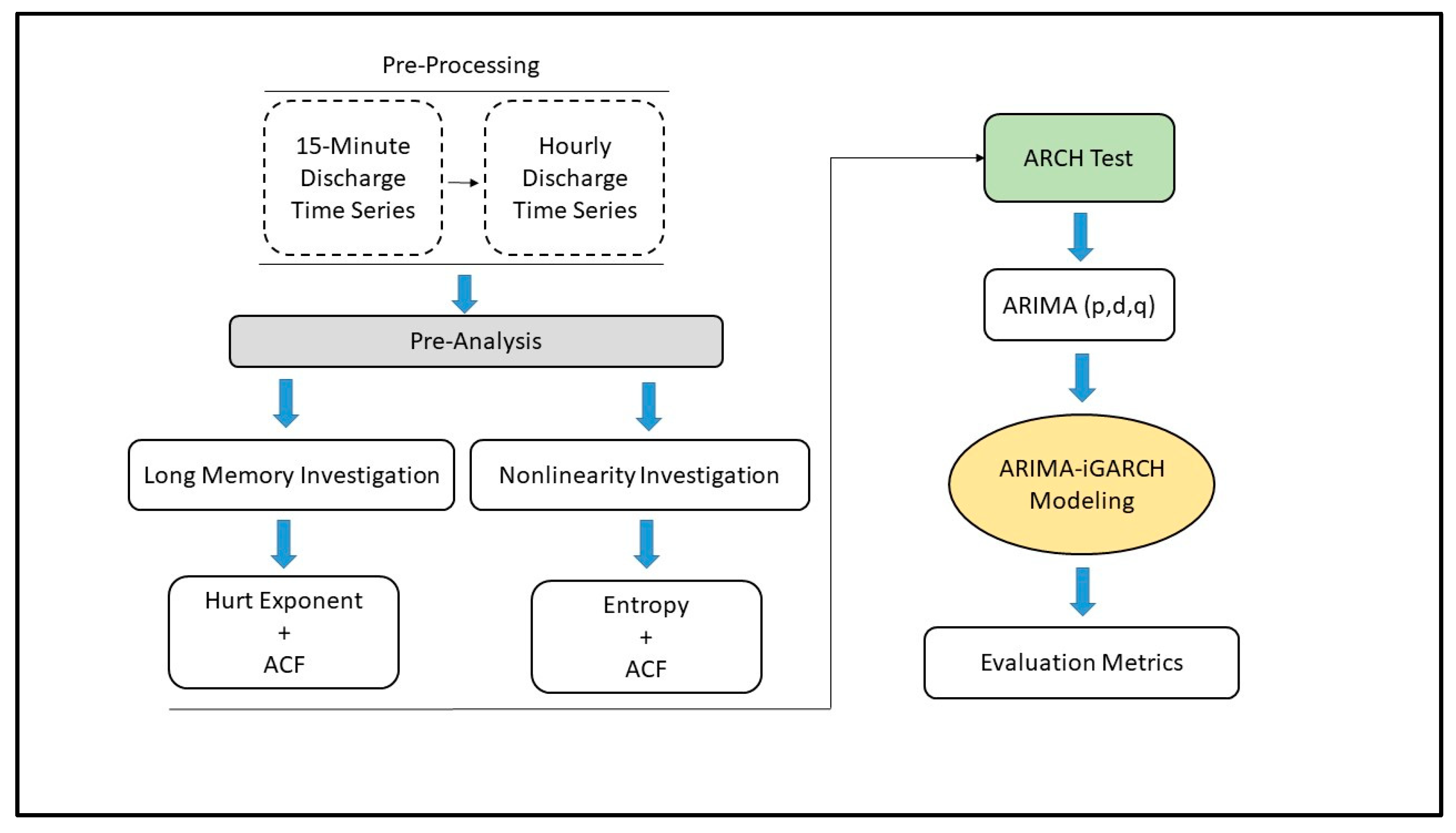
3. Methods

In the aim of finding the best-fitted model, we converted the 15 min step interval time series of streamflow to hourly time series by averaging the values of every four consecutive observations. This aggregation aimed to reduce noise, making the data more manageable for our modeling framework while potentially enhancing computational efficiency. Additionally, hourly aggregation smooths irregular fluctuations, improving model fitting and parameter stability. We determined the suitability of the ARIMA-iGARCH model for our studied time series data by developing the following systematic approach. This approach is outlined in the methodology flow chart presented in Figure 2.

3.1. Long Memory Investigation

Detecting long memory through ACF and Hurst exponent justified the inclusion of the GARCH structure, which is capable of modeling persistent variance.

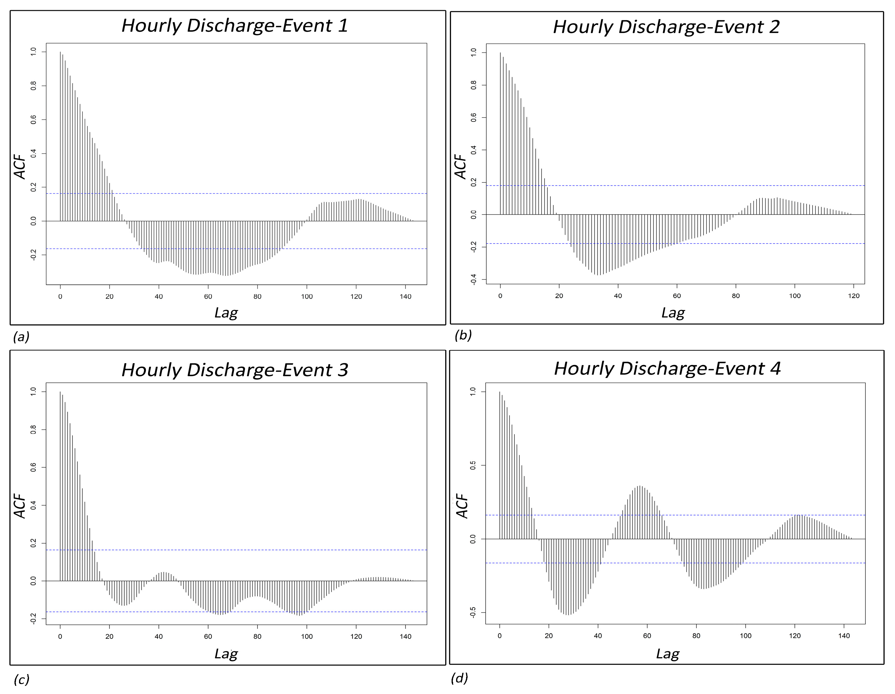
3.1.1. Autocorrelation Function (ACF)

In order to check the time series long memory, as the GARCH null hypothesis, we used ACF method in this study. Long memory represents the long-term autocorrelation between two observations in a time series [44]. ACF reveals how the correlation between two variables in a time series varies when comparing observations at different time lags [55]. It measures the stochastic process memory in a time domain with no further information about frequency content. Long memory in a time series can be detected using the ACF graph; if the ACF values decay to zero gradually, this indicates the presence of long memory [44]. The ACF equation is defined as follows:

$$R_X\left(\tau \right)=E\left[X_t{X}_{t+\tau }\right]=\left[{\displaystyle \frac{1}{T}}{\int }_{-{\displaystyle \frac{T}{2}}}^{{\displaystyle \frac{T}{2}}}{X}_t{X}_{T+\tau }dt\right]$$

(1)

where $R_X\left(\tau \right)$ is the autocorrelation function at time lag τ, X_t and X_(t+τ) are the signal at time t and t + τ, respectively. Expected value operator is represented by E, and T is the duration over which the integration is performed.

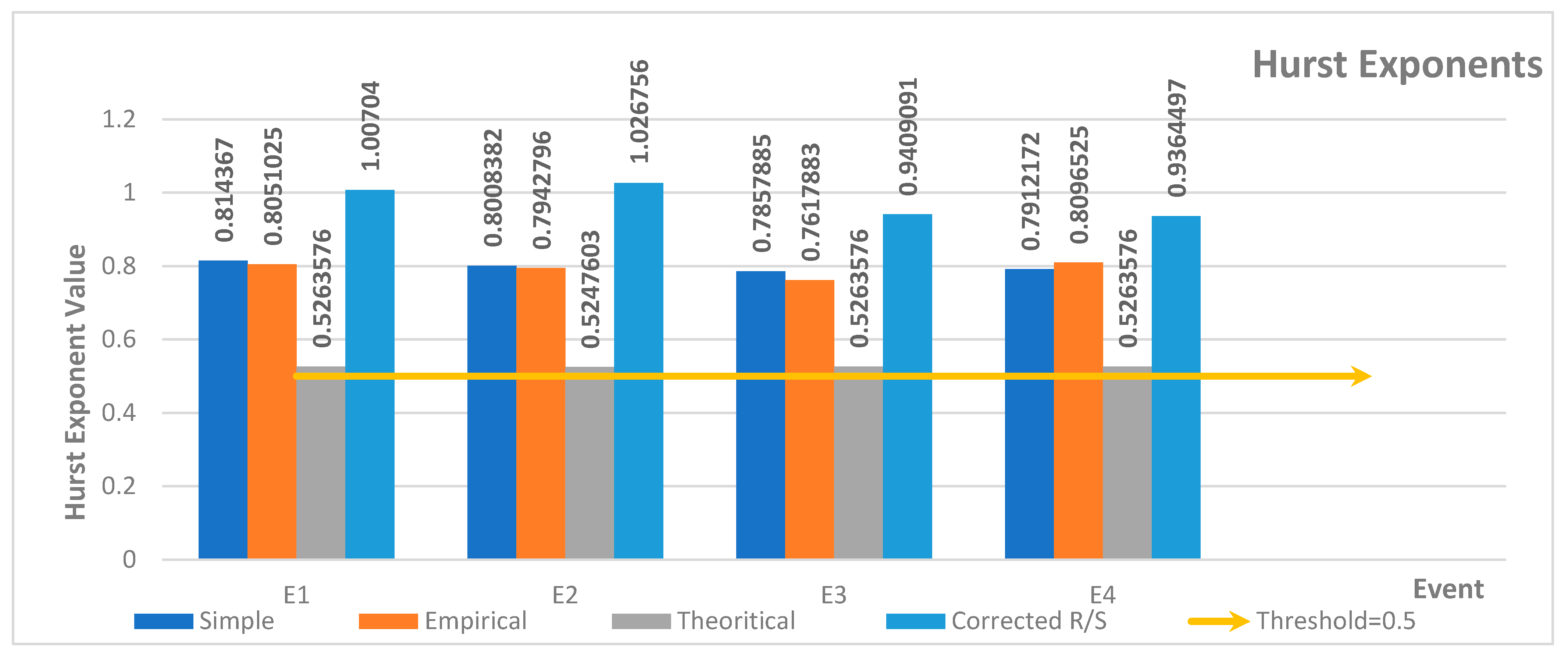
3.1.2. Rescaled Range Analysis (Hurst Exponent)

In the aim of long memory investigation, we used rescaled range analysis. This method was introduced by Hurst in 1951 [39] while he was working on dam dimensioning over the Nile river. Hurst exponent recognizes the presence of long memory in a time series by calculating the ratio of two parameters: (a) the distance between the maximum and minimum of the cumulative deviations from the mean and (b) standard deviation [63]. The main idea behind the rescaled range analysis method is that the range of the cumulative deviations from the mean of a time series should scale with the size of the data window [64]. The calculation of the ratio (R/S) is as shown below:

$${\displaystyle \frac{R\left(n\right)}{S\left(n\right)}}={\displaystyle \frac{1}{s}}{\sum }_{i=1}^s{\displaystyle \frac{R_s\left(n\right)}{S_s\left(n\right)}}$$

(2)

$$R_s\left(n\right)={max}_{1\le j\le n}\left(X_j\left(n\right)\right)-{min}_{1\le j\le n}\left(X_j\left(n\right)\right)$$

(3)

$$X_j\left(n\right)={\sum }_{i=1}^j\left(x_i-{x¯}_n\right) for j=\mathrm{1,2},\dots , n$$

(4)

$$S_s\left(n\right)=\sqrt{{\displaystyle \frac{{\sum }_{i=1}^j{\left(x_i-{x¯}_n\right)}^2}{n}}}$$

(5)

where ${x¯}_n$is the mean of time series. Finally, Hurst exponent is defined as follows:

$${\displaystyle \frac{R\left(n\right)}{S\left(n\right)}}={C_n}^H$$

(6)

where C is constant and H is the Hurst exponent, and it is usually determined by least square regression of rescaled ranges vs. n on a double logarithmic plot. Aligning with the aim of gaining a comprehensive analysis of the time series behavior, we used three types of Hurst exponents: simple, empirical, and theoretical. The simple Hurst exponent provides an initial estimate of long-term dependencies using rescaled range analysis method. The empirical Hurst exponent considers the observed properties and irregularities of the time series. In contrast, the theoretical Hurst exponent assesses how well the data matches theoretical predictions. For all of them, the Hurst exponent value of more than 0.5 acknowledges the long memory existence in the dataset.

3.2. Nonlinearity Investigation

The observed nonlinearity via ACF and entropy measures supports the use of a hybrid framework, allowing the model to account for nonlinear dynamics and improve prediction accuracy under volatile conditions.

3.2.1. Autocorrelation Function (ACF)

In addition to using the ACF to recognize the long memory, we used it also for detecting the nonlinearity patterns in this study. This method, which is detailed in the “Long memory Investigation” section (Section 3.1), analyses the correlation between the time series and its lagged values in the aim of assessing the nonlinear dependencies. Any deviations from the expected patterns in the ACF plot can indicate the presence of nonlinearity, thus complementing the other methods employed in this section. However, nonlinear means the relationship between variables in a time series cannot be presented by a straight line. In other words, it means that past values can affect the future values in a complex manner. The mathematical form of ACF is described in the previous sections.

3.2.2. Entropy

Aligned with the aim of discovering nonlinearity, we applied entropy method, one of the most well-known complexity measures. Complexity and chaos typically arise in nonlinear systems. They can be defined as a concept to characterize the dynamic patterns in a dataset [36]. Entropy can recognize the chance of point-to-point fluctuations in a time series. Higher value of entropy indicates higher degree of complexity, whereas more regularity would generate less entropy value [8]. We selected two kinds of entropy measures: Multiscale Entropy (MSE) and Permutation Entropy (PE). MSE measures the complexity over multiple temporal scales. It follows the variability at different resolutions. This makes MSE particularly well suited to the time series with long memory dependencies, which we dealt with in this study. On the other hand, PE analyses the temporal order of values in the aim of measuring system’s randomness. In comparison with MSE, PE is more sensitive to short-term dynamics.

MSE averages the data at different time scales to assess the complexity. Then, it applies sample entropy to each coarse-grained series. Sample entropy quantifies the predictability of the time series. The formula for the coarse-grained series at scale $\tau$ is as follows:

$$y_j^{\left(\tau \right)}={\displaystyle \frac{1}{\tau }}{\sum }_{i=\left(j-1\right)\tau +1}^{j\tau }{x}_i$$

(7)

where $x_i$ is the original time series and $y_j^{\left(\tau \right)}$ is the coarse-grained time series at scale $\tau$. On the other hand, PE measures complexity based on the order of values in the series, calculated as follows:

$$PE=-{\sum }_{p\in P}p log(p)$$

(8)

where p is the probability distribution of ordinal patterns in the embedded time series.

3.3. Autoregressive Moving Average (ARIMA)

In this study, we used ARIMA model for two purposes: Initially, we identified the best-fitting ARIMA model based on the minimum Akaike Information Criterion (AIC) following the Hyndman–Khandakar algorithm, which systematically combines unit root tests with maximum likelihood estimation and with the optimal parameters, on all four hourly discharge time series to test the ARCH test. The ARCH test results indicate significant ARCH effects, suggesting that GARCH model could effectively capture the time-varying volatility in our data. Then, by applying ARIMA, we obtained the best value of p, d, and q; the number of time lags; the degree of differencing; and the order of the moving average, respectively. Subsequently, we analyzed the residuals of the fitted ARIMA model to ensure that they resembled white noise, indicating that the model adequately captured the mean structure of the series. ARIMA is a data-driven model that is a hybrid of the autoregressive (AR) and moving average (MA) models. “AR” is the connection between a variable and its lagged value. “MA” is the linear connection between an observation and errors of previous observations. “I” is the difference between an object and previous ones in order to reach the stationary [65]. It shows that “I” will be zero in stationary time series. In this case, ARIMA changes to ARMA. In general, ARIMA uses a variation of the Hyndman–Khandakar algorithm [34], which combines unit root tests and minimization of the AICc and MLE. The structure of ARIMA is given by the following:

$$x_t={\delta }_1{x}_{t-1}^d+ {\delta }_p{x}_{t-p}^d+\dots + {\theta }_1{e}_{t-1}+ {\theta }_q{e}_{t-q}+ e_t+c$$

(9)

where $\delta$s is the parameter of autoregressive part and $\theta$s is the parameter of the moving average part. e represents the error terms. x^d is x differenced d times, and c is a constant.

3.4. Integrated Generalized Autoregressive Conditional Heteroskedasticity (iGARCH)

GARCH is a data-driven model, especially for the chaotic series variance modeling [66]. This option significantly enhances the accuracy of simulating streamflow forecast errors [67]. However, in the case dealing with persistent shocks or long-term dependence in the variance, the standard GARCH model may not fully follow the volatility persistence bounds. This is where iGARCH comes in to use its benefits. iGARCH is a type of GARCH model, specially defined to model the time series with permanent effect of volatility process shocks. The general mathematic forms of GARCH and iGARCH are defined as shown below:

For GARCH (r, s), it is the following:

$${\mathrm{C}\mathrm{o}\mathrm{n}\mathrm{d}\mathrm{i}\mathrm{t}\mathrm{i}\mathrm{o}\mathrm{n}\mathrm{a}\mathrm{l} \mathrm{m}\mathrm{e}\mathrm{a}\mathrm{n} \mathrm{e}\mathrm{q}\mathrm{u}\mathrm{a}\mathrm{t}\mathrm{i}\mathrm{o}\mathrm{n}: y}_t= \mu + {\epsilon }_t$$

(10)

where $y_t$ is the observed time series, $\mu$ is the mean, and ${\epsilon }_t$ is the error at time t.

Conditional Variance Equation is as follows:

$${\epsilon }_t=\gamma +{\sum }_{i=1}^r{\alpha }_i{\epsilon }_{t-i}+{\sum }_{j=1}^s{\beta }_j{e}_{t-j}^2$$

(11)

where ${\epsilon }_t=var\left(e_t\right|e_{t-1}, e_{t-2},\dots )$ is conditional variance of the current forecast error $e_t$, $\gamma$ is a constant term, and ${\alpha }_i$ and ${\beta }_j$ are the coefficients of ${\epsilon }_{t=i}$ and $e_{t-j}$, respectively. r and s are the orders of the conditional variance and the error term, respectively.

In general, GARCH model equations acknowledge that both the forecast error before multiple periods and their stochastic disturbance can affect the forecast error. This is one of the features of time-varying time series. For each event, the iGARCH model structure was specified individually through a trial-and-error process, guided by diagnostic checks of the ARIMA residuals and the observed persistence in volatility, allowing for appropriate selection of ARMA and iGARCH orders to best capture the dynamic behavior of each time series.

For iGARCH (r, s), it is defined as follows:

$${\sum }_{i=1}^p{\beta }_i+{\sum }_{i=1}^q{\alpha }_i=1$$

(12)

where $\alpha$ and $\beta$ are described as before.

3.5. Evaluation Metrics

3.5.1. Coefficient of Determination (R²)

The proportion of the variance in the dependent variable is calculated by $R^2$. Based on the total variance of the model’s outcomes, it indicates how well the observed outcomes are recreated by the model. $R^2=1$ means that the model perfectly forecasts the dependent variable, while $R^2=0$ means that the model cannot explain any of the variance. The formula of $R^2$ is as shown below:

$$R^2={\displaystyle \frac{{\sum }_{i=1}^N{\left(y_i-{y^}_i\right)}^2}{{\sum }_{i=1}^N{\left(y_i-y¯\right)}^2}}$$

(13)

where $y_i$ is the observation value, ${y^}_i$ is the predicted value, $y¯$ is the average of the observed values, and N is the total number of values in the time series.

3.5.2. Root Mean Squared Error (RMSE)

RMSE is the average amount of the errors between predicted and observed values. RMSE with lower amount shows the better model performance. It is defined as shown below:

$$RMSE=\sqrt{{\displaystyle \frac{{\sum }_{i=1}^N{\left(y_i-{y^}_i\right)}^2}{N}}}$$

(14)

where $y_i$ and ${y^}_i$ are the observed and predicted value, respectively, and N is the total number of datasets.

3.5.3. Mean Absolute Percentage Error (MAPE)

MAPE measures the average percentage difference between the predicted and observed values. It is scale independent and widely used to evaluate forecasting accuracy. A lower MAPE value indicates better model performance. MAPE is calculated as follows:

$$MAPE={\displaystyle \frac{100}{N}}{\sum }_{i=1}^N\left|{\displaystyle \frac{y_i-y_i^{^}}{y_i}}\right|$$

(15)

where $y_i$ is the observed value, $y_i^{^}$ is the predicted value, and N is the total number of observations.

3.5.4. Mean Absolute Error (MAE)

MAE represents the average magnitude of the errors between predicted and observed values without considering their direction. It is a linear score, meaning all individual differences are weighted equally. MAE is defined as follows:

$$MAE={\displaystyle \frac{1}{N}}{\sum }_{i=1}^N\left|y_i-y_i^{^}\right|$$

(16)

where $y_i$ and, $y_i^{^}$ are the observed and predicted values, respectively, and N is the number of observations.

3.5.5. Mean Bias Error (MBE)

MBE evaluates the average bias in the predictions by measuring the mean deviation of the predicted values from the actual values. It indicates whether the model tends to overestimate or underestimate. A value close to zero indicates unbiased predictions. The formula is given by the following:

$$MBE={\displaystyle \frac{1}{N}}{\sum }_{i=1}^N\left(y_i-y_i^{^}\right)$$

(17)

where $y_i^{^}$ is the predicted value and $y_i$ is the observed value and N is the number of observations.

3.5.6. Nash–Sutcliffe Efficiency (NSE)

NSE is a normalized statistic that determines the relative magnitude of the residual variance compared to the measured data variance. An NSE of 1 indicates a perfect match between modeled and observed data, while values less than zero indicate poor model performance. It is defined as follows:

$$NSE=1-{\displaystyle \frac{{\sum }_{i=1}^N{\left(y_i-y_i^{^}\right)}^2}{{\sum }_{i=1}^N{\left(y_i-y_i^{¯}\right)}^2}}$$

(18)

where $y_i$ is the observed value, $y_i^{^}$ is the predicted value, $y^{¯}$ is the mean of the observed values, and N is the number of observations.

3.5.7. Index of Agreement (d-Index)

The d-index is a standardized measure developed to overcome the insensitivity of NSE to differences in the observed and predicted means and variances. It ranges between 0 (no agreement) and 1 (perfect agreement). The formula is as follows:

$$d=1-{\displaystyle \frac{{\sum }_{i=1}^N{\left(y_i-y_i^{^}\right)}^2}{{\sum }_{i=1}^N{\left(\left|y_i^{^}-y^{¯}\right|+\left|y_i-y^{¯}\right|\right)}^2}}$$

(19)

where $y_i$, $y_i^{^}$, and $y^{¯}$ are the observed value, predicted value, and mean of observed values, respectively.

3.5.8. Evaluation Approach

Given the short duration and limited data points of each event, model validation was conducted on the full available dataset after parameter estimation, where model parameters were selected based on criteria such as AIC and likelihood measures. This approach aligns with the study’s focus on data-limited conditions and supports assessing the model’s generalizability across distinct events.

4. Results and Discussion

4.1. Time Series Interval Conversion

Switching from a 15 min to an hourly time series led to qualitatively improved model results. This enhancement can be attributed to several factors:

• Noise reduction and signal-to-noise ratio growth are the results from data aggregation, so it will allow us to follow the trends and patterns more clearly.
• Additionally, hourly data can better adapt to the temporal dynamics of many modeling methods.
• Furthermore, by increasing the time interval to hourly, we could decrease the computational load in order to use the data preparation techniques more effectively.
• Statistically, hourly aggregation reduces autocorrelation at short lags and improves model stability, making it more suitable for capturing conditional heteroskedasticity patterns such as those modeled by iGARCH.
• Finally, hourly data leads to more robust statistical estimates.

4.2. Long Memory

To investigate the long memory, two different approaches were used. The Hurst exponent analysis as a mathematical method and ACF as a graphical method. Overall, the results of both methods indicate the presence of strong long memory in four events. This persistence demonstrates the data is not independent over time. Thus, past values can affect the future values.

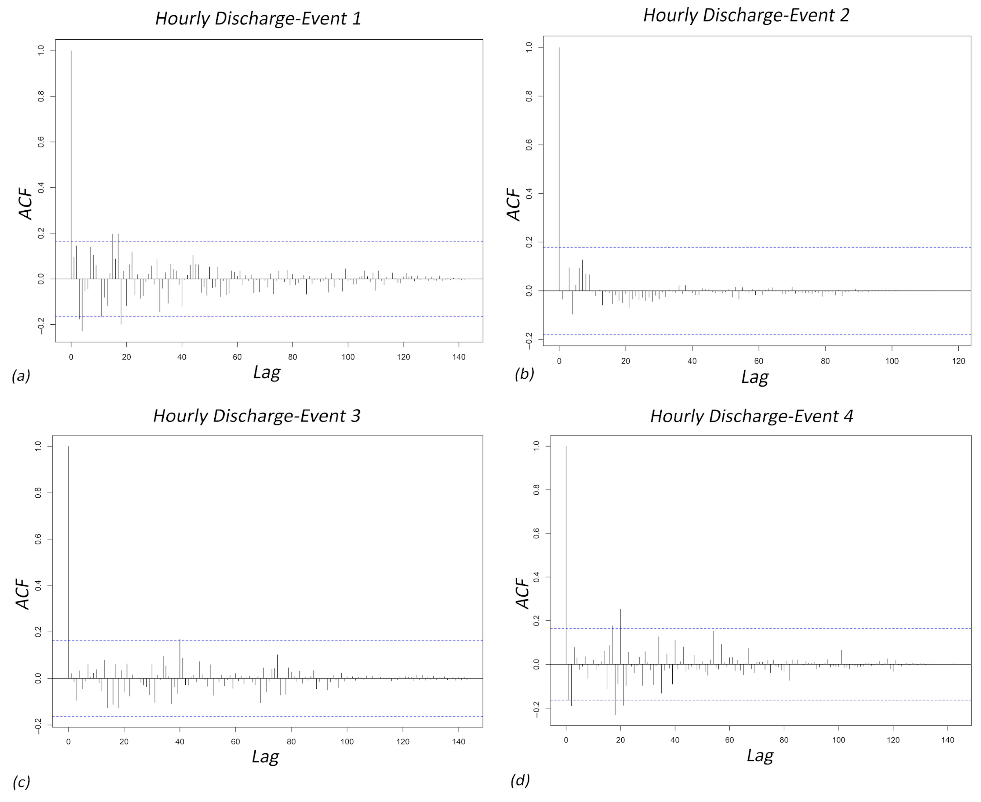
4.2.1. Autocorrelation Function (ACF)

For all events, ACF plots are mapped in Figure 4a–d. The graphs present a slow decay in autocorrelation values, demonstrating long memory presence. Comparing the events, Event 1 shows more pronounced long memory. This is evident from the slower decay of autocorrelation values by the time lag increasing. Almost 14% of the ACF values of Event 1 remained significantly above the threshold of statistical significance, which is a considerable amount. In contrast, there is a more rapid decrease for the other three events, indicating shorter memory process. We can say that Event 1 data is influenced by previous values over a longer period. This could be due to different reasons, such as the catchment characteristics, antecedent moisture conditions, or the nature of the precipitation event that generated the discharge. For instance, a stronger long memory effect can be a result from a prolonged rainfall.

4.2.2. Hurst Exponent

The Hurst exponent values are shown in Figure 3 with the threshold line for long memory value. It can be seen that the simple R/S vary from 0.7858 to 0.8144, indicating a tendency towards persistence in the data, in such a way that higher simple R/S propose a more pronounced long-range dependence. Specifically, Event 1 has the highest simple R/S in contrast with Event 3 with the lowest, for the strongest and weakest long memory existence, respectively. Additionally, the range of the empirical values, from 0.7618 to 0.8097, displays a slightly different pattern. It has the highest value of 0.8097 for Event 4 while the lowest value of 0.7618 for Event 3. This difference can be related to the differences in data characteristics or measurement techniques used for empirical estimation. On the other hand, the theoretical values for events are around 0.526. This relatively stable value indicates the existence of a long memory. Additionally, the corrected R over S are almost 1 and even more. These high amounts acknowledge a positive correlation between past and future values. In general, Event 1 has the strongest long memory. This result reveals that while Event 4 might experience more fluctuations, it does not necessarily imply long memory.

4.3. Nonlinearity

In this study, the ACF and entropy method were employed with the aim of evaluating nonlinearity. All four events exhibit a strong nonlinear behavior. This indicates that the time series are following a complex pattern that includes curves, sudden changes, and varying rates of increase or decrease over time.

4.3.1. ACF

As the graphical method to assess the time series nonlinearity, the ACF method was applied. The results are shown in Figure 4a–d. They exhibit the patterns deviated from the behavior expected under linear models. These patterns present a nonlinear dynamic within the data. Nonlinearity can have various sources, like no uniform distribution of rainfall, varying soil moisture conditions, or changes in land surface characteristics that affect runoff processes. ACF plots that approve more than just a simple linear relationship affect the successive discharge values. Based on the ACF graphs, Events 3 and 4 have more noticeable periodic fluctuations with alternating positive and negative correlations. Specially, the Event 4 pattern shows remarkable periodicity in the lag, 16, 45, 70, and 109, which could be from the interactions between different hydrological processes, such as rapid shifts between infiltration and runoff.

4.3.2. Entropy

For characterizing the dataset dynamics, we apply entropy methods. The results reveal nonlinearity of dynamical properties across the events. The Multiscale Entropy (MSE) values are 1.493, 0.273, 1.144, and 1.796, respectively. The maximum MSE related to Event 4, indicating the greatest complexity. This high intensity can be clearly seen in the ACF graph in Figure 4d as a periodic behavior, and it came into view of a periodic trend. Conversely, a minimum MSE value of 0.273 determined for Event 2 confirms the data’s lower variability. In terms of ranking, Event 1 and Event 3 follow the second and third ranks, suggesting more moderate underlying patterns. For Permutation Entropy (PE), the values are 0.727, 0.612, 0.668, and 0.754, in sequence. Based on the results, Event 4 shows the most chaotic pattern. In contrast, the lowest amount of PE is observed for Event 2, reflecting simpler dynamics. There is a remarkable gap in the MSE and PE values for Event 2, likely due to less complexity, which aligns with the autocorrelation function (ACF) graphs showing reduced correlation in the data. The comparison between MSE and PE demonstrates an unpredictable and nonlinear nature for events. The results obtained from PE are completely aligned with the results of MPE. It proves that the most and the lowest uncertainty are related to Event 4 and 2, respectively. The difference between the MSE and PE could be set down to differences in their different analytical approach: MSE captures the complexity over multiple scales, while PE focuses on the temporal order of the data. Overall, these results highlight the lack of consistency or fixed pattern in time series complexity.

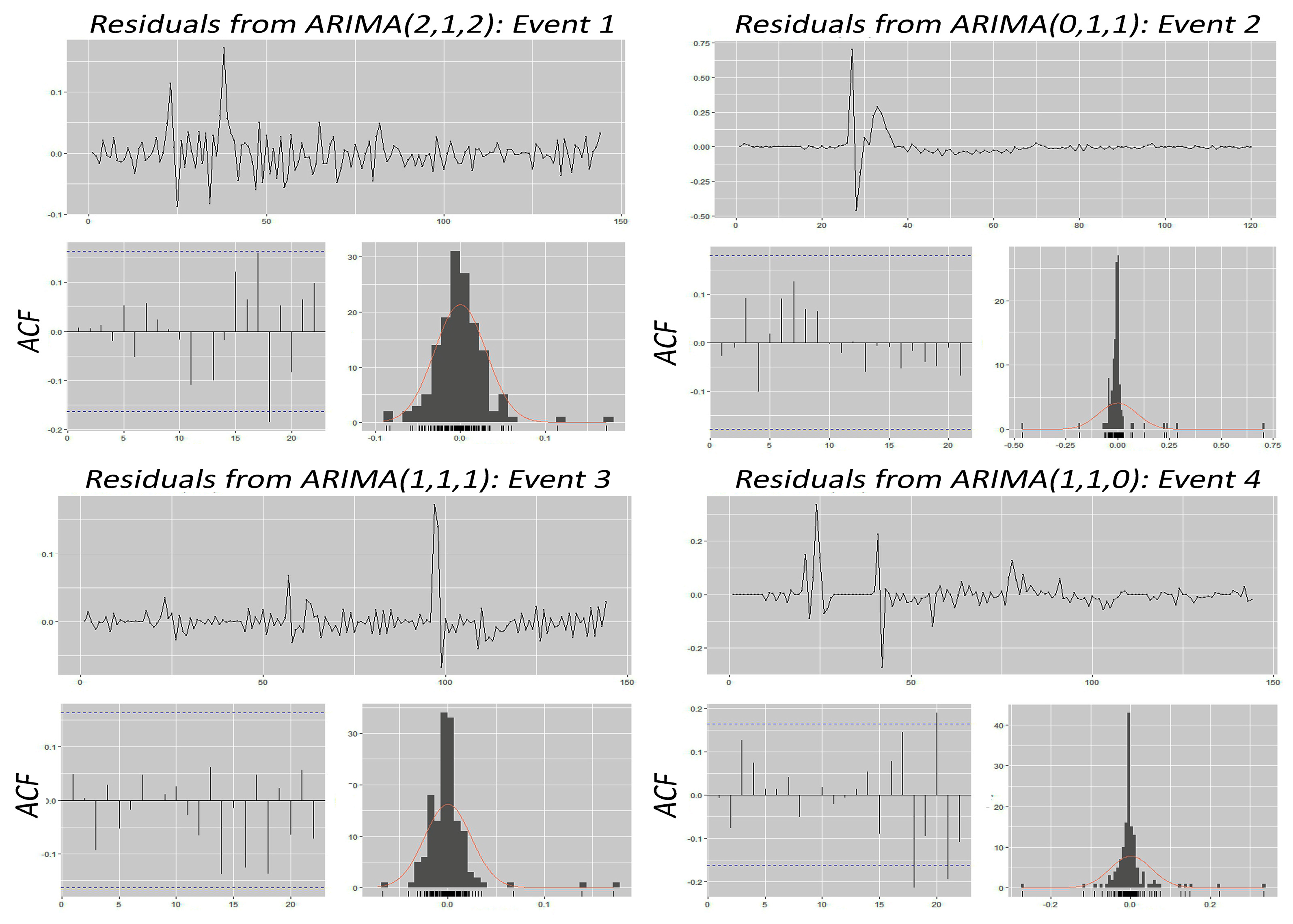
4.4. ARIMA

ARIMA is used for covering two aims: First, we investigate the ARCH effect. Based on the results, all four datasets display a strong ARCH effect in their underlying pattern. Figure 5 shows the residuals of the time series after applying ARIMA, plotted against time. As it can be seen, the residuals are scattered around the y-line equal to zero and are completely spread, suggesting the presence of an ARCH effect. This dispersion highlights that the residual variance is time-dependent and confirms the use of the GARCH family to capture volatility. In the next step, we use ARIMA again to achieve the best value for calculating the iGARCH specification. In this step, the AIC and BIC criteria are used to determine the optimal order of the model. This can help achieve the most accurate model fit by balancing model complexity and predictive performance, ensuring that overfitting is minimized while capturing the key dynamics of the time series. Figure 6 contains residual pattern graphs, the ACF of residuals, and the graph of density, providing strong evidence of the well-fitted ARIMA, as it successfully addresses autocorrelation, meets normality assumptions, and produces residuals with a stable pattern. The first linear graph showing a stable pattern indicates that the residuals are homoscedastic without any systematic trends over time. This stability confirms the model has effectively managed to capture the time series dynamics without leaving any discernible structure. Furthermore, the ACF plot reveals that all residuals fall within the confidence interval bands, indicating that there are no significant autocorrelations left in the residuals and suggesting that the model has successfully captured the temporal dependencies in the data. Additionally, the last graph shows that the residuals follow a normal distribution. This is crucial because one of the assumptions of ARIMA models is that residuals should be normally distributed, as this allows for reliable parameter estimation, valid hypothesis testing, and accurate confidence intervals in forecasting. Event 3 shows the highest AIC and BIC along with the smallest RMSE, indicating a strong model fit. In contrast, the highest RMSE and relatively poor AIC and BIC are related to Event 2, suggesting less accurate predictions due to higher variability. Despite the entropy results proving more predictable dynamics for Event 2, the results of ARIMA show more error in the residuals. This conflict might be the ARIMA sensitivity to short-term patterns like sudden changes within the data. Referring to Figure 2, there is a jump at the fortieth hour within Event 2. While ARIMA effectively captures trends and seasonality, the specific structure of the data has appeared as a sharp shift and may require more autoregressive terms. Additionally, the high accuracy of the ARIMA for Event 3 can be attributed to the ARIMA’s good performance with more gradual changes rather than sudden shifts, which aligns well with the stable changes in Event 3 (refer to Figure 2). Similarly, when comparing Events 1 and 4, ARIMA shows better fitting for Event 1, with a single significant jump, whereas Event 4, with two major jumps, presents greater challenges for the model.

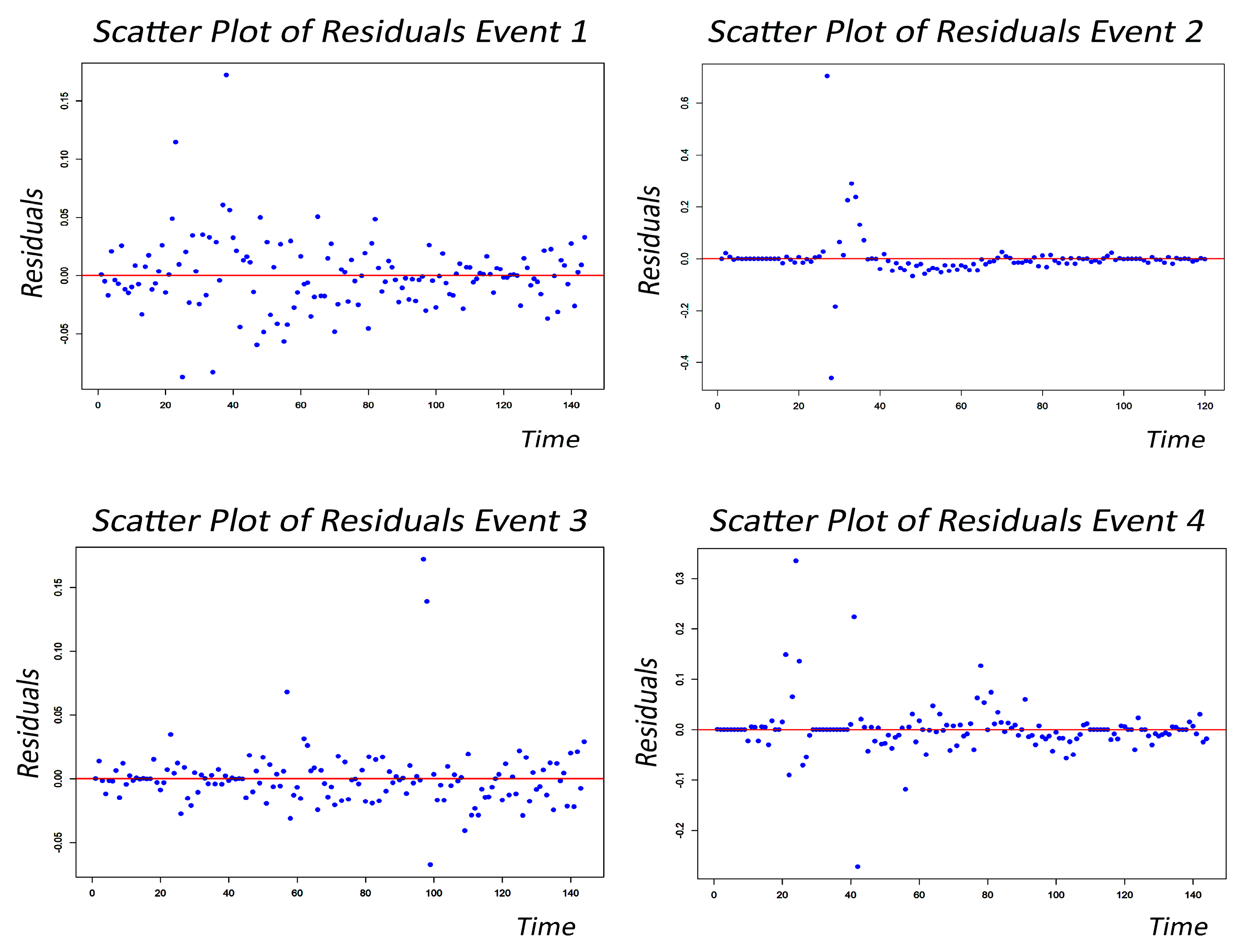
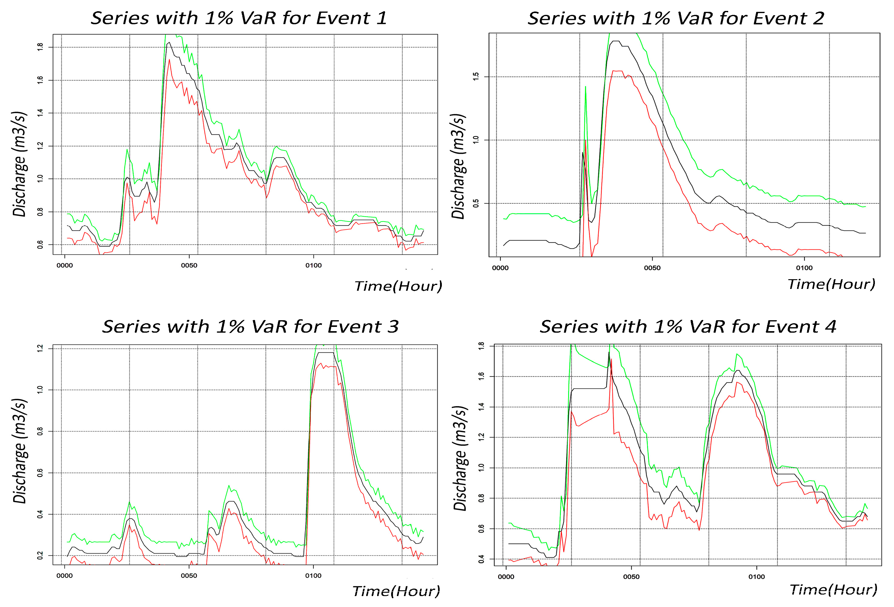
4.5. ARIMA-iGARCH

Dealing with short-term datasets for training the artificial neural network models, following limited data quantity, can be a challenge. We propose an innovative ARIMA-iGARCH model that addresses this limitation. This model provides richer information about the time series underlying dynamics, accounting for long memory and nonstationary shifts. ARIMA is not well suited in accurately simulating the pattern featured with clustering volatility and temporal dependency. However, it is effective in modeling the time series mean. GARCH, in contrast, effectively preserves these traits by capturing fluctuations and time-dependent variations, leading to considerable forecasting capabilities. We employ GARCH with various parameters to fit the most accurate model, and the iGARCH is introduced as a specialized approach to better capture fluctuation dynamics.

Table 2. ARIMA-iGARCH model orders and performance metrics.

Event	iGARCH Order	Mu	Alpha1	Beta1	LogLikelihood	AIC	Nyblom Stability Test Statistic	Pearson Goodness-of-Fit Test (p-Value)
E1	1,1	0.713	0.133	0.867	319.527	−4.368	0.871	0.0001979
E2	0,1	0.168	-	1.000	117.244	−1.904	0.271	6.355 × 10−65
E3	0,1	0.209	-	1.000	333.855	−4.567	0.314	0.00001478
E4	1,1	0.515	0.086	0.914	252.520	−3.452	0.566	3.25 × 10−15

starts with the iGARCH order and shows the order (1,1) for Event 1 and 4 while the order (0,1) for Event 2 and 3. That is the reason the alpha specification is absent for Event 2 and 3, suggesting a reduced volatility effect compared with Event 1 and 4. However, Event 1 has the highest mu value at 0.713, indicating a higher mean return, while Event 2 with the lowest value at 0.0168. The high mu rate can be reflected to a more substantial underlying trend or drift in the time series in the data compared to Event 2. The iGARCH results and mu values align with the earlier findings from MSE, PE, and Hurst exponent analysis, where Event 1 reveals the highest complexity and the strongest persistence, while Event 2 displays the smoothest patterns. The Nyblom stability test further distinguishes these aspects, indicating that Event 1 also has the highest stability with a statistic of 0.871, suggesting reliable parameter estimates. In contrast, Event 2, despite its smoother patterns and lower complexity, has a lower Nyblom statistic of 0.271, indicating reduced stability and suggesting less consistent parameter estimates. The summary of model performance across events reveals notable differences. Based on the LogLikelihood values, Event 3 has the highest fit with 333.855, while Event 2 has the lowest at 117.244. This is mirrored by the AIC values, where Event 3 again fares best with the lowest AIC of −4.567, suggesting a more efficient model, whereas Event 2 has the highest AIC at −1.904. Finally, the p-values of the Pearson Goodness-of-Fit test show that Event 4 achieves the most favorable fit with a p-value of 3.25 × 10⁻¹⁵, contrasting with Event 1’s p-value of 0.0001979, which also indicates a good fit but less so than Event 4. Finally, Figure 7 shows the comparison between the line predicted by the ARIMA-iGARCH model and the observed data, representing ±1% variance around the model’s predictions. This figure approves the model’s effectiveness in capturing the real-world fluctuations and patterns, validating its performance and reliability.

4.6. Evaluation Metrics

As each flood event includes a limited number of observations, model evaluation was performed on the same dataset used for parameter tuning. This practical approach reflects real-world constraints and still allows for meaningful performance assessment across distinct hydrological scenarios.

To comprehensively evaluate the model’s performance under these conditions, we evaluate the performance of the ARIMA-iGARCH model using a diverse set of metrics to capture both accuracy and robustness. In addition to the commonly used RMSE, MAPE, and R², we incorporate MAE and MBE to assess the average magnitude and direction of prediction errors, respectively. Furthermore, the NSE and d-index are used to evaluate the model’s ability to reproduce observed variability across the entire range of flow values. A summary of these evaluation metrics for all events is presented in

Table 3. Evaluation metrics.

Event	RMSE	MAPE	R2	MAE	MBE	NSE	d-Index
E1	0.031	2.044	0.99	0.02	−0.003	0.99	0.997
E2	0.091	4.769	0.96	0.03	−0.006	0.96	0.99
E3	0.023	3.77	0.99	0.01	−0.002	0.99	0.998
E4	0.052	2.601	0.98	0.02	−0.004	0.98	0.995

. The results reveal consistently low RMSEs and MAPEs across all events, indicating high predictive precision. Particularly, Event 3 stands out with the lowest RMSE and highest NSE, highlighting its accuracy and reliability in replicating observed flows. The MBE values, close to zero, confirm the absence of systematic bias in the model’s predictions, and d-index values consistently above 0.99, ranging from 0.995 to 0.998, suggest excellent agreement with the observed data. To go beyond numerical validation, we also analyzed the ACF plot of residuals to assess the presence of autocorrelation. The results showed that residuals remained within the confidence bounds and exhibited no significant autocorrelation, indicating that the model successfully captured the mean structure and adapted to time-varying volatility, particularly during high-flow events. These findings are visually supported by the residual autocorrelation plots shown in Figure 8. This adaptability is a key strength over traditional ARIMA or standalone GARCH models. The consistency of the model’s performance across contrasting events further underlines its robustness under different hydrological conditions, confirming its suitability for operational forecasting. By integrating multiple evaluation layers, accuracy, bias, variability capture, and stability, this analysis convincingly demonstrates the model’s effectiveness in handling complex hydrological dynamics.

5. Conclusions

Training artificial neural networks for short-term discharge modeling faces challenges due to nonlinearity, nonstationarity, seasonality, and randomness in streamflow data. This study introduces a data-driven hybrid model, ARIMA-iGARCH, combining ARIMA’s trend-following strengths with iGARCH’s capacity to handle time-dependent fluctuations and volatility. The model is applied to hourly discharge data from four significant flood events on the German Schwarzbach River.

Key findings include the following:

• Regarding long memory, the Hurst exponent method shows strong long-memory effects (values >0.5) across all events, with Event 1 exhibiting the strongest correlation.
• Regarding nonlinearity, the entropy analysis reveals notable fluctuations in hourly discharge, indicating a non-constant pattern. Event 4, with its periodic nature, displays the highest nonlinearity, underscoring the need for a fluctuation-sensitive model.
• The detection of long memory and nonlinear patterns in the streamflow data justified the application of a hybrid ARIMA-iGARCH model, which combines linear modeling for the mean and nonlinear conditional heteroskedasticity for the variance. These features improve the model’s accuracy by capturing persistent dependencies and volatility clustering that simpler models might overlook.
• Regarding the ARIMA model performance, the ARIMA model captures average value responses to nonlinearity, enhancing modeling accuracy. However, its sensitivity to sudden jumps (notably in Event 2) can lead to residual errors. Optimizing iGARCH specifications using ARIMA reduces forecast errors.
• Regarding the ARIMA-iGARCH model performance, the ARIMA-iGARCH model effectively models volatility and time-dependent fluctuations, achieving its best performance in Event 3 with high R² and low RMSE. This model is reliable for addressing variance and improving short-term hydrological predictions.
• The ARIMA-iGARCH model improves flood forecasting and discharge assessment, making it valuable for water management. Its ability to capture variability supports early-warning systems and strengthens resilience to hydrological extremes, contributing to effective land and water management.
• This modeling approach offers scientific advancement while addressing urgent practical needs in early-warning systems, paving the way for more adaptive and resilient hydrological infrastructure under uncertain conditions.

In the current study, the modeling framework incorporates both the mean and the variance components of the streamflow series to capture central tendency and volatility. Future research may build upon this by integrating additional stochastic elements that reflect higher-order statistical characteristics, such as skewness or kurtosis. This extension could enhance the model’s capacity to represent the probabilistic behavior of discharge, particularly under highly variable or extreme hydrological conditions.

In addition, further development could focus on improving the model’s sensitivity to sharp peaks in discharge time series. Incorporating advanced pattern recognition strategies or adaptive rule-based mechanisms may allow the model to more accurately capture the timing and magnitude of flood peaks, which are critical for operational forecasting and early-warning systems.

References

- Bai, X.; Zhao, W. Impacts of climate change and anthropogenic stressors on runoff variations in major river basins in China since 1950. Sci. Total. Environ. 2023, 898, 165349. [Google Scholar] [CrossRef]
- MacDonald, G.; Godbout, A.; Gillcash, B.; Cairns, S. Volume-preserving Neural Networks. In Proceedings of the 2021 International Joint Conference on Neural Networks (IJCNN), Shenzhen, China, 18–22 July 2021; pp. 1–9. [Google Scholar]
- Wang, W.; Van Gelder, P.H.A.J.M.; Vrijling, J.K.; Ma, J. Testing and modelling autoregressive conditional heteroskedasticity of streamflow processes. Nonlinear Process. Geophys. 2005, 12, 55–66. [Google Scholar] [CrossRef]
- Giri, F.; Devercelli, M. Chaos arising from the hydrological behaviour of a floodplain river during the last century. River Res. Appl. 2022, 39, 241–254. [Google Scholar] [CrossRef]
- Lai, Y.; Dzombak, D.A. Use of the Autoregressive Integrated Moving Average (ARIMA) Model to Forecast Near-Term Regional Temperature and Precipitation. Weather. Forecast. 2020, 35, 959–976. [Google Scholar] [CrossRef]
- Li, Y.; Huang, C.; Ding, L.; Li, Z.; Pan, Y.; Gao, X. Deep learning in bioinformatics: Introduction, application, and perspective in the big data era. Methods 2019, 166, 4–21. [Google Scholar] [CrossRef]
- Marwan, N.; Donges, J.F.; Donner, R.V.; Eroglu, D. Nonlinear time series analysis of palaeoclimate proxy records. Quat. Sci. Rev. 2021, 274, 107245. [Google Scholar] [CrossRef]
- Bhasme, P.; Bhatia, U. Improving the interpretability and predictive power of hydrological models: Applications for daily streamflow in managed and unmanaged catchments. J. Hydrol. 2024, 628, 130421. [Google Scholar] [CrossRef]
- Naimy, V.; Haddad, O.; Fernández-Avilés, G.; El Khoury, R.; Segovia, J.E.T. The predictive capacity of GARCH-type models in measuring the volatility of crypto and world currencies. PLoS ONE 2021, 16, e0245904. [Google Scholar] [CrossRef]
- Wong, W.M.; Lee, M.Y.; Azman, A.S.; Rose, L.A.F. Development of Short-term Flood Forecast Using ARIMA. Int. J. Math. Model. Methods Appl. Sci. 2021, 15, 68–75. [Google Scholar] [CrossRef]
- Fathian, F.; Fard, A.F.; Ouarda, T.B.; Dinpashoh, Y.; Nadoushani, S.M. Modeling streamflow time series using nonlinear SETAR-GARCH models. J. Hydrol. 2019, 573, 82–97. [Google Scholar] [CrossRef]
- Izadi, A.; Zarei, N.; Nikoo, M.R.; Al-Wardy, M.; Yazdandoost, F. Exploring the potential of deep learning for streamflow forecasting: A comparative study with hydrological models for seasonal and perennial rivers. Expert Syst. Appl. 2024, 252, 124139. [Google Scholar] [CrossRef]
- Naji, A.S.M.; Yaziz, S.R.; Zakaria, R.; Mohamad, N.N.; Radi, N.F.A. Gold price forecasting using ARIMA-GARCH model during COVID-19 pandemic outbreak. AIP Conf. Proc. 2024, 2895, 090018. [Google Scholar] [CrossRef]
- Pashazadeh, A.; Javan, M. Comparison of the gene expression programming, artificial neural network (ANN), and equivalent Muskingum inflow models in the flood routing of multiple branched rivers. Theor. Appl. Clim. 2020, 139, 1349–1362. [Google Scholar] [CrossRef]
- Wang, H.; Song, S.; Zhang, G.; Ayantoboc, O.O. Predicting daily streamflow with a novel multi-regime switching ARIMA-MS-GARCH model. J. Hydrol. Reg. Stud. 2023, 47. [Google Scholar] [CrossRef]
- HLNUG. Nauheim gauge (ID 23980353) in Hesse, Germany: Discharge Data [Data Set]. Database of Hessian Agency for Nature Conservation, Environment and Geology (Hessisches Landesamt für Naturschutz, Umwelt und Geologie). 2023. Available online: https://www.hlnug.de/static/pegel/wiskiweb3/webpublic/#/overview/Durchfluss/station/41361/Nauheim/ (accessed on 5 June 2023).
- Khazaeiathar, M.; Hadizadeh, R.; Attar, N.F.; Schmalz, B. Daily Streamflow Time Series Modeling by Using a Periodic Autoregressive Model (ARMA) Based on Fuzzy Clustering. Water 2022, 14, 3932. [Google Scholar] [CrossRef]
- Alzubaidi, L.; Zhang, J.; Humaidi, A.J.; Al-Dujaili, A.; Duan, Y.; Al-Shamma, O.; Santamaría, J.; Fadhel, M.A.; Al-Amidie, M.; Farhan, L. Review of deep learning: Concepts, CNN architectures, challenges, applications, future directions. J. Big Data 2021, 8, 53. [Google Scholar] [CrossRef]
- Khazaiee, M.; Khalili, K.; Behmanesh, J. Investigating the relationship between physical characteristics of watersheds and nonlinearity of daily streamflow processes. Int. J. Water 2018, 12, 141. [Google Scholar] [CrossRef]
- Choi, E.; Bahadori, M.T.; Kulas, J.A.; Schuetz, A.; Stewart, W.F.; Sun, J. RETAIN: An Interpretable Predictive Model for Healthcare using Reverse Time Attention Mechanism. Adv. Neural Inf. Process. Syst. 2016, 29. Available online: http://arxiv.org/abs/1608.05745 (accessed on 21 March 2025).
- Khand, K.; Senay, G.B. Evaluation of streamflow predictions from LSTM models in water- and energy-limited regions in the United States. Mach. Learn. Appl. 2024, 16, 100551. [Google Scholar] [CrossRef]
- Roodschild, M.; Sardiñas, J.G.; Will, A. A new approach for the vanishing gradient problem on sigmoid activation. Prog. Artif. Intell. 2020, 9, 351–360. [Google Scholar] [CrossRef]
- Rawat, D.; Mishra, P.; Ray, S.; Warnakulasooriya, H.H.F.; Sati, S.P.; Mishra, G.; Alkattan, H.; Abotaleb, M. Modeling of rainfall time series using NAR and ARIMA model over western Himalaya, India. Arab. J. Geosci. 2022, 15, 1–26. [Google Scholar] [CrossRef]
- Samantaray, S.; Sahoo, P.; Sahoo, A.; Satapathy, D.P. Flood discharge prediction using improved ANFIS model combined with hybrid particle swarm optimisation and slime mould algorithm. Environ. Sci. Pollut. Res. 2023, 30, 83845–83872. [Google Scholar] [CrossRef]
- Wang, X.; Qin, Y.; Wang, Y.; Xiang, S.; Chen, H. ReLTanh: An activation function with vanishing gradient resistance for SAE-based DNNs and its application to rotating machinery fault diagnosis. Neurocomputing 2019, 363, 88–98. [Google Scholar] [CrossRef]
- Lee, K.; Lee, K.; Shin, J.; Lee, H. Overcoming catastrophic forgetting with unlabeled data in the wild. In Proceedings of the IEEE International Conference on Computer Vision, Seoul, Republic of Korea, 27 October 2019; pp. 312–321. [Google Scholar] [CrossRef]
- Moura, R.; Mendes, A.; Cascalho, J.; Mendes, S.; Melo, R.; Barcelos, E. Predicting Flood events with Streaming Data: A Preliminary Approach with GRU and ARIMA. In Optimization, Learning Algorithms and Applications. OL2A 2023. Communications in Computer and Information Science 1981; Pereira, A.I., Mendes, A., Fernandes, F.P., Pacheco, M.F., Coelho, J.P., Lima, J., Eds.; Springer: Cham, Switzerland, 2024; pp. 319–332. [Google Scholar] [CrossRef]
- Parsaie, A.; Ghasemlounia, R.; Gharehbaghi, A.; Haghiabi, A.; Chadee, A.A.; Nou, M.R.G. Novel hybrid intelligence predictive model based on successive variational mode decomposition algorithm for monthly runoff series. J. Hydrol. 2024, 634, 131041. [Google Scholar] [CrossRef]
- Sharma, A.K.; Punj, P.; Kumar, N.; Das, A.K.; Kumar, A. Lifetime Prediction of a Hydraulic Pump Using ARIMA Model. Arab. J. Sci. Eng. 2024, 49, 1713–1725. [Google Scholar] [CrossRef]
- Mo, R.; Xu, B.; Zhong, P.-A.; Dong, Y.; Wang, H.; Yue, H.; Zhu, J.; Wang, H.; Wang, G.; Zhang, J. Long-term probabilistic streamflow forecast model with “inputs–structure–parameters” hierarchical optimization framework. J. Hydrol. 2023, 622, 129736. [Google Scholar] [CrossRef]
- Srivastava, N.; Hinton, G.; Krizhevsky, A.; Salakhutdinov, R. Dropout: A Simple Way to Prevent Neural Networks from Overfitting. J. Mach. Learn. Res. 2014, 15, 1929–1958. [Google Scholar]
- Pandit, M.; Gaur, M.K.; Kumar, S. Artificial Intelligence and Sustainable Computing; Pandit, M., Gaur, M.K., Kumar, S., Eds.; Springer Nature: Dordrecht, GX, The Netherlands, 2023. [Google Scholar]
- Chukwueloka, E.; Nwosu, A. Modelling and Prediction of Rainfall in the North-Central Region of Nigeria Using ARIMA and NNETAR Model. In Climate Change Impacts on Nigeria, Springer Climate; Egbueri, J.C., Ighalo, J.O., Pande, C.B., Eds.; Springer: Cham, Switzerland, 2023; pp. 91–114. [Google Scholar] [CrossRef]
- Hyndman, R.J.; Khandakar, Y. Automatic Time Series Forecasting: The forecast Package for R. J. Stat. Softw. 2008, 27, 1–22. [Google Scholar] [CrossRef]
- Nazeri-Tahroudi, M.; Ramezani, Y.; De Michele, C.; Mirabbasi, R. Bivariate Simulation of Potential Evapotranspiration Using Copula-GARCH Model. Water Resour. Manag. 2022, 36, 1007–1024. [Google Scholar] [CrossRef]
- Dos Santos, C.F.G.; Papa, J.P. Avoiding Overfitting: A Survey on Regularization Methods for Convolutional Neural Networks. ACM Comput. Surv. 2022, 54, 1–25. [Google Scholar] [CrossRef]
- Brito, G.R.A.; Villaverde, A.R.; Quan, A.L.; Pérez, M.E.R. Comparison between SARIMA and Holt–Winters models for forecasting monthly streamflow in the western region of Cuba. SN Appl. Sci. 2021, 3, 1–12. [Google Scholar] [CrossRef]
- Golpaygani, A.; Keshtkar, A.; Mashhadi, N.; Hosseini, S.M.; Afzali, A. Optimal selection of cost-effective biological runoff management scenarios at watershed scale using SWAT-GA tool. J. Hydrol. Reg. Stud. 2023, 49. [Google Scholar] [CrossRef]
- Hurst, H.E. Long-Term Storage Capacity of Reservoirs. Trans. Am. Soc. Civ. Eng. 1951, 116, 770–808. [Google Scholar] [CrossRef]
- Li, Y.; Ding, L.; Gao, X. On the Decision Boundary of Deep Neural Networks. arXiv 2018, arXiv:1808.05385. [Google Scholar] [CrossRef]
- Mohanty, A.; Sahoo, B.; Kale, R.V. A hybrid model enhancing streamflow forecasts in paddy land use-dominated catchments with numerical weather prediction model-based meteorological forcings. J. Hydrol. 2024, 635, 131225. [Google Scholar] [CrossRef]
- Abbasi, A.; Khalili, K.; Behmanesh, J.; Shirzad, A. Estimation of ARIMA model parameters for drought prediction using the genetic algorithm. Arab. J. Geosci. 2021, 14, 841. [Google Scholar] [CrossRef]
- Chen, X.; Jiang, Z.; Cheng, H.; Zheng, H.; Cai, D.; Feng, Y. A novel global average temperature prediction model—Based on GM-ARIMA combination model. Earth Sci. Inform. 2024, 17, 853–866. [Google Scholar] [CrossRef]
- Wu, M.; Liu, P.; Liu, L.; Zou, K.; Luo, X.; Wang, J.; Xia, Q.; Wang, H. Improving a hydrological model by coupling it with an LSTM water use forecasting model. J. Hydrol. 2024, 636. [Google Scholar] [CrossRef]
- Khan, M.M.H.; Mustafa, M.R.U.; Hossain, M.S.; Shams, S.; Julius, A.D. Short-Term and Long-Term Rainfall Forecasting Using ARIMA Model. Int. J. Environ. Sci. Dev. 2023, 14, 292–298. [Google Scholar] [CrossRef]
- Noh, S.-H. Analysis of Gradient Vanishing of RNNs and Performance Comparison. Information 2021, 12, 442. [Google Scholar] [CrossRef]
- Retike, I.; Bikše, J.; Kalvāns, A.; Dēliņa, A.; Avotniece, Z.; Zaadnoordijk, W.J.; Jemeljanova, M.; Popovs, K.; Babre, A.; Zelenkevičs, A.; et al. Rescue of groundwater level time series: How to visually identify and treat errors. J. Hydrol. 2022, 605, 127294. [Google Scholar] [CrossRef]
- Wong, W.M. Flood Prediction using ARIMA Model in Sungai Melaka, Malaysia. Int. J. Adv. Trends Comput. Sci. Eng. 2020, 9, 5287–5295. [Google Scholar] [CrossRef]
- Ning, Y.Z.; Musa, S. Stream Flow Forcasting on Pahang River by Time Series Models, ARMA, ARIMA and SARIMA. Recent Trends Civ. Eng. Built Environ. 2023, 4, 331–341. [Google Scholar]
- Madhushani, C.; Dananjaya, K.; Ekanayake, I.; Meddage, D.; Kantamaneni, K.; Rathnayake, U. Modeling streamflow in non-gauged watersheds with sparse data considering physiographic, dynamic climate, and anthropogenic factors using explainable soft computing techniques. J. Hydrol. 2024, 631, 130846. [Google Scholar] [CrossRef]
- Nounou, M.N.; Bakshi, B.R.; Walczak, B. Multiscale Methods for Denoising and Compression; Elsevier Science BV: Amsterdam, The Netherlands, 2000; pp. 119–150. [Google Scholar] [CrossRef]
- Modarres, R.; Ouarda, T. Modeling rainfall–runoff relationship using multivariate GARCH model. J. Hydrol. 2013, 499, 1–18. [Google Scholar] [CrossRef]
- Sarhadi, A.; Modarres, R.; Vicente-Serrano, S.M. Dynamic compound droughts in the Contiguous United States. J. Hydrol. 2023, 626, 130129. [Google Scholar] [CrossRef]
- Cheng, S. Heterogeneity In Stock Price Forecasting-Based on the ARIMA-GARCH Model And PCA-LSTM Model. Highlights Sci. Eng. Technol. 2024, 88, 39–46. [Google Scholar] [CrossRef]
- Kandukuri, K. The Rainfall Forecast Models Analysis and Their Volatility. Int. J. Stat. Reli-Abil. Eng. 2023, 9, 450–460. [Google Scholar]
- Archibong, M.E.; Essi, I.D. Modelling Petroleum Prices between Garch and Intergeated Garch, (Igarch). J. Adv. Math. Comput. Sci. 2021, 36, 95–101. [Google Scholar] [CrossRef]
- Caporale, G.M.; Pittis, N.; Spagnolo, N. IGARCH models and structural breaks. Appl. Econ. Lett. 2003, 10, 765–768. [Google Scholar] [CrossRef]
- Mo, C.; Lai, S.; Yang, Q.; Huang, K.; Lei, X.; Yang, L.; Yan, Z.; Jiang, C. A comprehensive assessment of runoff dynamics in response to climate change and human activities in a typical karst watershed, southwest China. J. Environ. Manag. 2023, 332, 117380. [Google Scholar] [CrossRef]
- HLNUG. Nauheim Gauge (ID 23980353) in Hesse, Germany: Station Information. Hessian Agency for Nature Con-servation, Environment and Geology (Hessisches Landesamt für Naturschutz, Umwelt und Geologie). 2023. Available online: https://www.hlnug.de/static/pegel/wiskiweb3/webpublic/#/overview/Durchfluss/station/41361/Nauheim/stationInfoHlnug (accessed on 20 May 2025).
- LUBW: Deutsches Gewässerkundliches Jahrbuch DGJ (German Hydrological Yearbook) Rheingebiet, Teil I 2009 (Rhine Area, Part 1 2009). Landesanstalt für Umwelt, Messungen und Naturschutz Baden-Württemberg (in German). Karlsruhe. 2011. Available online: https://pd.lubw.de/38631 (accessed on 22 March 2024).
- DWD. Precipitation data from station Frankfurt/M. (Flughfn.) ID 1420 (Frankfurt Airport) [Data Set]. Germany’s National Meteorological Service (Deutscher Wetterdienst). 2023. Available online: https://cdc.dwd.de/portal/ (accessed on 5 June 2023).
- HLNUG. Overview About Water Level Monitoring Stations in Hesse. Hessian Agency for Nature Conservation, Envi-ronment and Geology (Hessisches Landesamt für Naturschutz, Umwelt und Geologie). 2022. Available online: https://www.hlnug.de/static/pegel/wiskiweb3/webpublic/#/overview/Wasserstand (accessed on 23 September 2022).
- Burud, N.B.; Kishen, J.C. Investigation of long memory in concrete fracture through acoustic emission time series analysis under monotonic and fatigue loading. Eng. Fract. Mech. 2023, 277, 108975. [Google Scholar] [CrossRef]
- Gao, S.; Zhang, S.; Huang, Y.; Han, J.; Zhang, T.; Wang, G. A hydrological process-based neural network model for hourly runoff forecasting. Environ. Model. Softw. 2024, 176, 106029. [Google Scholar] [CrossRef]
- Karimi, H.; Derr, T.; Tang, J. Characterizing the Decision Boundary of Deep Neural Networks. arXiv 2019, arXiv:1912.11460. [Google Scholar] [CrossRef]
- Le, M.T.; Le, H.M.H.; Nguyen, H.Q.; Pham, L.N.N. Geopolitical Risk, Economic Uncertainty, and Market Volatility Index Impact on Energy Price. Eng. Proc. 2025, 97, 36. [Google Scholar] [CrossRef]
- Bollerslev, T. Generalized autoregressive conditional heteroskedasticity. J. Econom. 1986, 31, 307–327. [Google Scholar] [CrossRef]