Article

Modeling the Dynamics of the Jebel Zaghouan Karst Aquifer Using Artificial Neural Networks: Toward Improved Management of Vulnerable Water Resources

by
Emna Gargouri-Ellouze
1,*,
Tegawende Arnaud Ouedraogo
2,
Fairouz Slama
1,
Jean-Denis Taupin
3,*,
Nicolas Patris
3 and
Rachida Bouhlila
1
1
Laboratory of Modelling in Hydraulics and Environment (LMHE), LR99ES19, National Engineering School of Tunis (ENIT), University of Tunis El Manar, Tunis 2092, Tunisia
2
Société du Canal de Provence (SCP), CEDEX 05, Le Tholonet, CS 70064, 13182 Aix-en-Provence, France
3
HydroSciences Montpellier, University of Montpellier, IRD, CNRS, IMT Mines-Alès, Montpellier, France
*
Authors to whom correspondence should be addressed.
Hydrology 2025, 12(10), 250; https://doi.org/10.3390/hydrology12100250
Submission received: 14 July 2025 / Revised: 18 September 2025 / Accepted: 23 September 2025 / Published: 26 September 2025

Abstract

Karst aquifers are critical yet vulnerable water resources in semi-arid Mediterranean regions, where structural complexity, nonlinearity, and delayed hydrological responses pose significant modeling challenges under increasing climatic and anthropogenic pressures. This study examines the Jebel Zaghouan aquifer in northeastern Tunisia, aiming to simulate its natural discharge dynamics prior to intensive exploitation (1915–1944). Given the fragmented nature of historical datasets, meteorological inputs (rainfall, temperature, and pressure) were reconstructed using a data recovery process combining linear interpolation and statistical distribution fitting. The hyperparameters of the artificial neural network (ANN) model were optimized through a Bayesian search. Three deep learning architectures—Multi-Layer Perceptron (MLP), Convolutional Neural Network (CNN), and Long Short-Term Memory (LSTM)—were trained to model spring discharge. Model performance was evaluated using Kling–Gupta Efficiency (KGE′), Nash–Sutcliffe Efficiency (NSE), and R2 metrics. Hydrodynamic characterization revealed moderate variability and delayed discharge response, while isotopic analyses (δ18O, δ2H, 3H, 14C) confirmed a dual recharge regime from both modern and older waters. LSTM outperformed other models at the weekly scale (KGE′ = 0.62; NSE = 0.48; R2 = 0.68), effectively capturing memory effects. This study demonstrates the value of combining historical data rescue, ANN modeling, and hydrogeological insight to support sustainable groundwater management in data-scarce karst systems.

Graphical Abstract

1. Introduction

Karst aquifers are essential components of the global water supply, providing approximately 25% of the world’s drinking water and supporting diverse agricultural needs [1,2,3]. These aquifers, formed mainly through the dissolution of carbonate rocks, exhibit a complex and highly heterogeneous network of flow paths. They are also characterized by significant variations in permeability [4,5,6,7]. The inherent geological and hydrological properties of karst systems are distinguished by their anisotropy, heterogeneity, and nonlinear subsystems [8,9,10]. Due to the considerable variability in hydraulic parameters of karst systems, such as conductivity and storage, a substantial challenge for numerical modeling, also known as the Karst Modeling Challenge or KMC, has emerged [4,5,11]. To address this challenge, hydrogeological modeling is a fundamental tool for the characterization of water resources dynamics within karst systems, facilitating improved management, development, and planning [12]. Karst modeling can broadly be categorized into lumped and physical parameter models [4,13,14,15]. Lumped models are utilized to understand the temporal variability of hydrodynamic behavior, offering insights into water movement patterns within the karst system [4,9,16,17,18]. Physical parameter models provide a detailed examination of the physical properties governing the system’s behavior, which enable a more comprehensive understanding of aquifer functioning [5,15,19,20,21,22]. Table 1 presents the various modeling approaches with their main advantages, disadvantages, and limitations.
Moreover, it is important to underscore that the selection of a modeling approach is contingent on multiple considerations, including but not limited to: the extent and quality of available data [23], geomorphology, and karst features specific to the study area [7], hydrodynamic functioning [24], climatic conditions [25] and the objectives of the investigation [9]. Ref. [4] suggested the integration of diverse methodologies to enhance the modeling of karst formations; nonetheless, this endeavor may introduce added intricacies and constrain its practical applicability.
In addition, the choice of the modeling approach is more complex and challenging when historical data is stored in printed documents, which must be digitized and pre-processed. This problem is emphasized in the challenge and innovation launched by many initiatives, i.e., ReHydrate (“Historical hydrological observations are often stored in printed documents and volumes of archives worldwide. This not only makes them practically inaccessible and unusable for modern hydrological studies but also puts them at risk of permanent loss due to the deterioration of their medium. In addition to the intrinsic value of rescuing past observations, having access to historical data is essential for understanding changes in the hydrological cycle and its extremes, which appear to be increasingly characterizing recent decades in several parts of the world. Several data rescue initiatives exist, but the efforts are highly fragmented in space and time.”) (REtrieve historical HYDRologic dATa & Estimates, https://iahs.info/Initiatives/Scientific-Decades/helping-working-groups/, accessed on 22 September 2025), which aims to preserve and leverage historical data to meet current and future challenges in water resource management [26].
Artificial Neural Networks (ANNs), considered as lumped models, have emerged in the recent decade as a prominent tool in karst hydrodynamic modeling [24,27,28,29,30,31,32]. ANNs are recognized for their capability to forecast hydrological outcomes without a detailed comprehension of the complex karst geometry; thereby simplifying the modeling process while addressing the inherent hydrogeological challenges of karst systems effectively [33,34,35,36,37]. In fact, ANNs can autonomously establish input-output relationships, offer a promising avenue for karst aquifer modeling despite the challenges associated with their “black box” nature and the extensive data requirements for training [24,38,39,40]. Through the efficient application of neural network methodologies, there is a potential for significant advancements in the effectiveness and efficiency of modeling karst aquifers, thereby contributing to the sustainable management and conservation of these vital water resources. Indeed, many karst systems are vulnerable and overexploited, risks which are amplified by climate change. These issues are particularly pronounced in the Jebel Zaghouan karst system in Tunisia, where it has been the main water drinking resource since the Roman era and has been encountering such a concerning situation since 1945 [41,42]. Since 1943, the karst has been subject to increasing anthropogenic pressure due to intensified pumping, highlighting the challenge of sustainable water management amidst growing demand and environmental changes. In consequence, Jebel Zaghouan karst is a crucial system to study. In addition, the study of Jebel Zaghouan karst systems presents further advantages, including the availability of both quantitative and qualitative data, as well as historical raw data series.
Table 1. Karst Modeling Approaches.
Modeling CategoryModelAuthorsAdvantagesDisadvantagesLimitations
Statistical and Regression ModelsLogistic Regression Model (LRM)[43] Handle both continuous and discrete variablesOversimplify karst complex relationshipsClear linear relationship
Conceptual ModelsKARSTMODGARDENIARCD Seasonal[9,14]Simplify the hydrological processInadequate for spatial heterogeneitySimple systems
Data Driven and Machine Learning ModelsData Mining Models (ANFIS, Fuzzy Logic, ANNs)[2]Flexible models Nonlinear RelationshipsData-intensive can be subjectiveData dependency (limited/noisy data)
ANNs (MLP/CNN/LSTM
/NARX)
[24]Efficient in learning spatial/temporal featuresRequire substantial computational resourcesNeed for high-quality and quantity of data
Support Vector Regression (SVR)[44]Effective in high-dimensional spacesSensitive to hyperparameter settingsCareful tuning of parameters
Physical-Based/Hydrodynamic ModelsMODFLOW[45,46]Handle groundwater flow processesMay require simplification of karst featuresPorous media flow
KarstFLOW[47]Directly simulate physical processesRequire detailed and hard-to-obtain system dataHigh computational demand
Empirical and Stochastic ModelsEmpirical Models[48]Simple to implement; requires less dataLimited predictive capability, Restrictive applicabilityReproducibility
Stochastic Models[49]Uncertainty and variability handling, limited data, constraints on time, and few computational resources.Numerous hypotheses on karst network configuration Complex to set up and interpretReplicability
Jebel Zaghouan karst system has already been modeled twice by reservoir models (lumped models) [41] and in [50] with KarstMod [14].
The model of [41] is characterized by four reservoirs: balance, transfer, aquifer, and karst conduits. The main inputs of the model are rainfall and evapotranspiration. The output of the model is the total discharge. It was developed using historical data from 1915 to 1962, with a calibration period from 1915 to 1927 prior to aquifer exploitation and validated from 1958 to 1962. Ref. [41] concluded that the model effectively simulates and monitors karst hydrodynamics, offering valuable capabilities to forecast water reserves and discharge responses in real-time, thus serving as a significant tool for managing and studying karst water resources.
Ref. [51] employed KarstMod to model the rainfall-discharge relationships of karst springs at daily and hourly time steps, as well as to analyze the hydrodynamics of the compartments represented in the model. The simulations successfully reproduced the model’s structure, with acceptable amplitude estimates across the entire time series. However, some flood events were underestimated, and while the simulated recession dynamics closely matched the observed data, the model consistently struggled to replicate rapid recession rates. This limitation was identified as a key factor affecting the overall performance of the simulations.
The main objective of this study is to deepen our understanding of the hydrological processes within the Jebel Zaghouan karst system, a critical resource that has been overexploited but lacks recent and updated studies. This research aims to address the challenges of assessing the hydrodynamic behavior of the karst system by utilizing historical raw data. For this purpose, we compare different data-driven modeling approaches using ANNs, and we evaluate the relevance of these approaches. This paper focuses on the natural karst behavior whose knowledge depends on the reconstruction and preservation of data prior to its exploitation. This foundational understanding is essential for informing future restoration efforts and establishing a sustainable management framework for the system.

2. Materials and Methods

This study aims to characterize the natural hydrodynamic behavior of the Jebel Zaghouan karst aquifer prior to anthropogenic exploitation. Before the development of water abstraction infrastructure, such as galleries and boreholes, the aquifer exhibited a natural functioning that was intrinsically linked to hydroclimatic variables, including precipitation, air temperature, and atmospheric pressure [41].
The methodological framework (Figure 1) comprises five main steps: (i) compilation and digitization of historical data (1915–1944) on precipitation, temperature, atmospheric pressure, and spring discharge; (ii) data gap-filling and reconstruction using both statistical interpolation techniques and autoregressive models based on artificial neural networks; (iii) analysis of the aquifer’s hydrodynamics through the examination of spring discharge time series, including flow duration analysis, autocorrelation (to assess memory effects), and cross-correlation (to evaluate response times); (iv) modeling of karst spring discharge using three deep learning architectures—Multilayer Perceptron (MLP), Convolutional Neural Network (CNN), and Long Short-Term Memory (LSTM). This stage involves model calibration, hyperparameter optimization via Bayesian techniques, and performance evaluation at daily and weekly time scales; (v) analysis and comparison of the model outputs to assess predictive performance and underlying hydrological processes.

2.1. Study Area

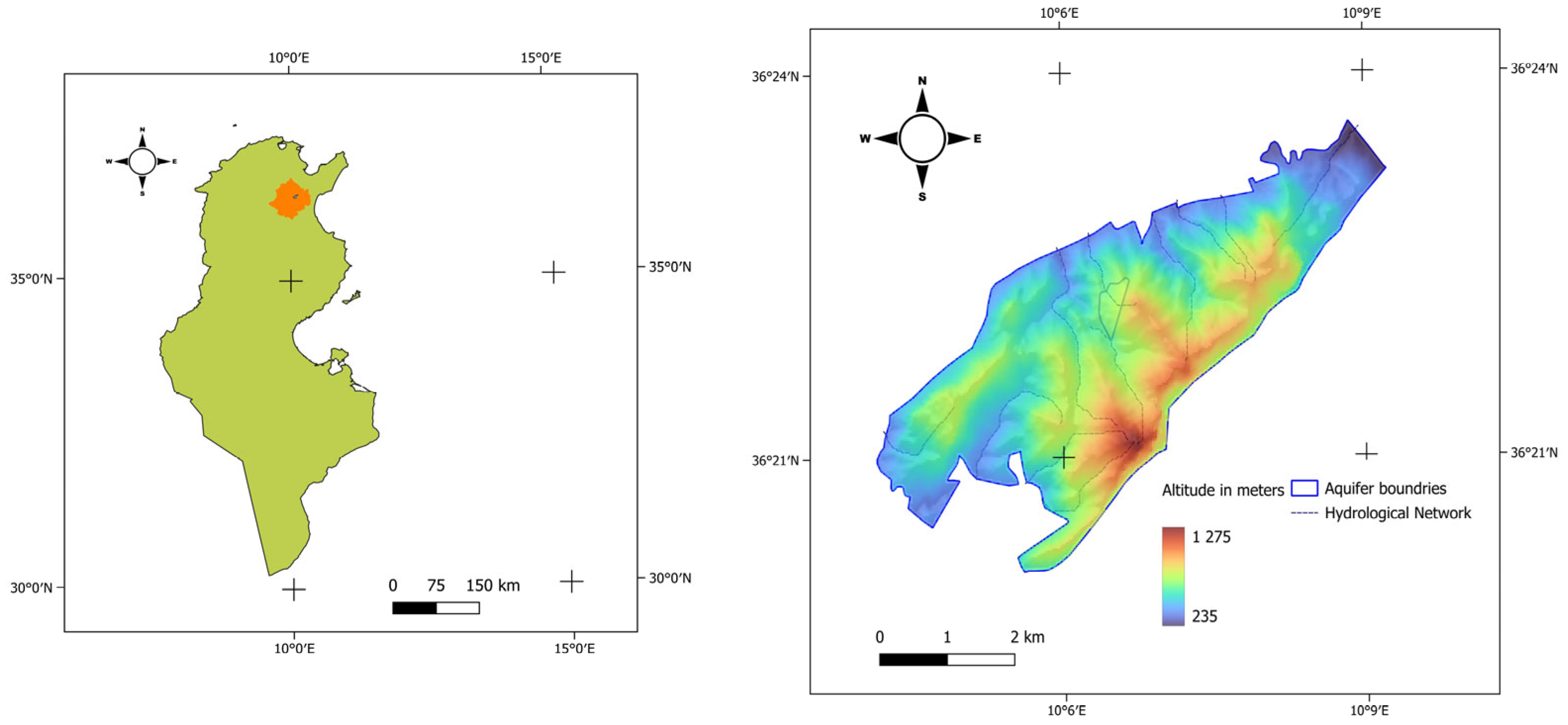
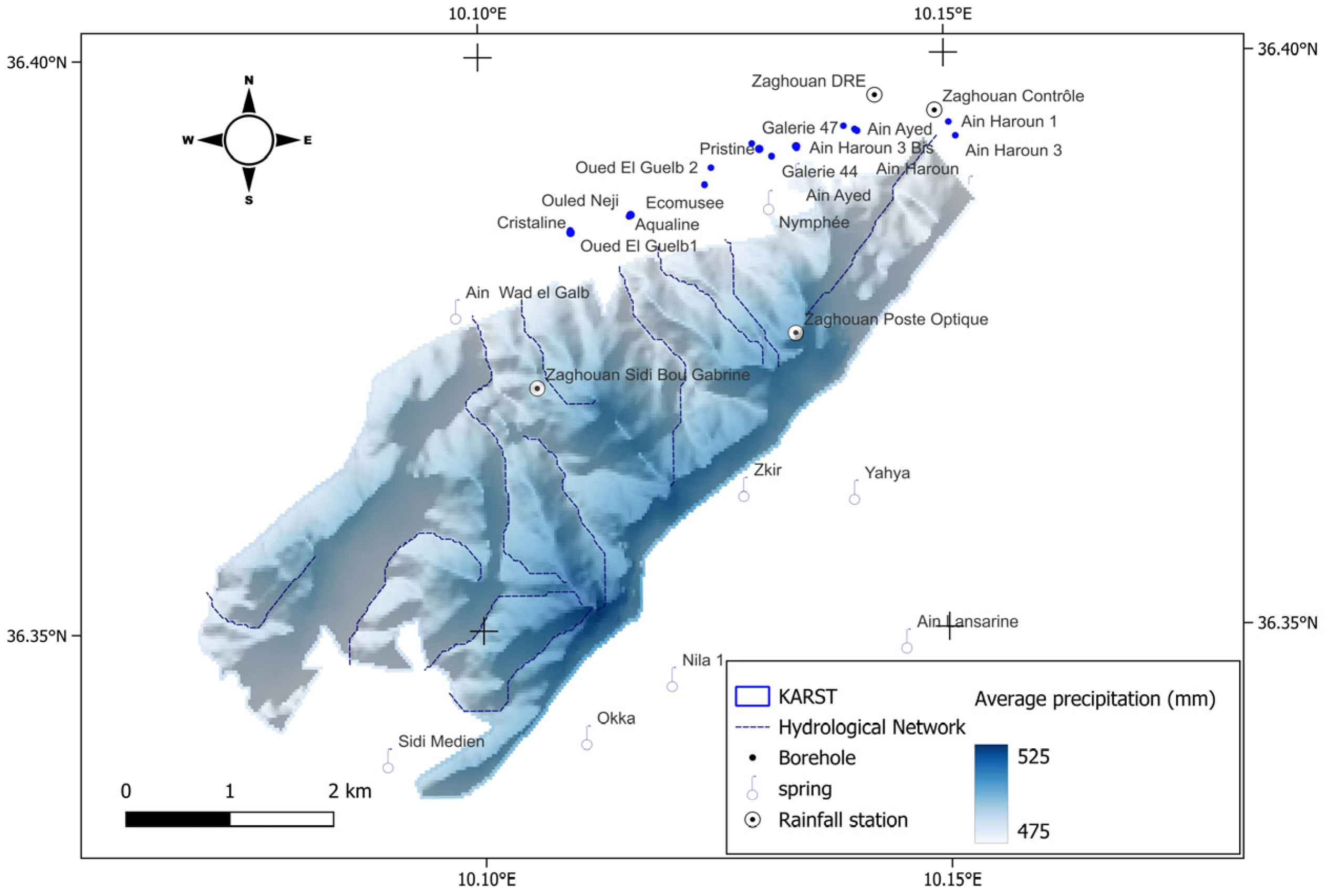
The Jebel Zaghouan karst aquifer is located approximately 50 km south of Tunis in Tunisia. It is distinguished by its significant Jurassic formation within the Zaghouan massif, encompassing roughly 19.6 km2 (Figure 2).

2.1.1. Geological Context, Aquifer Geometry

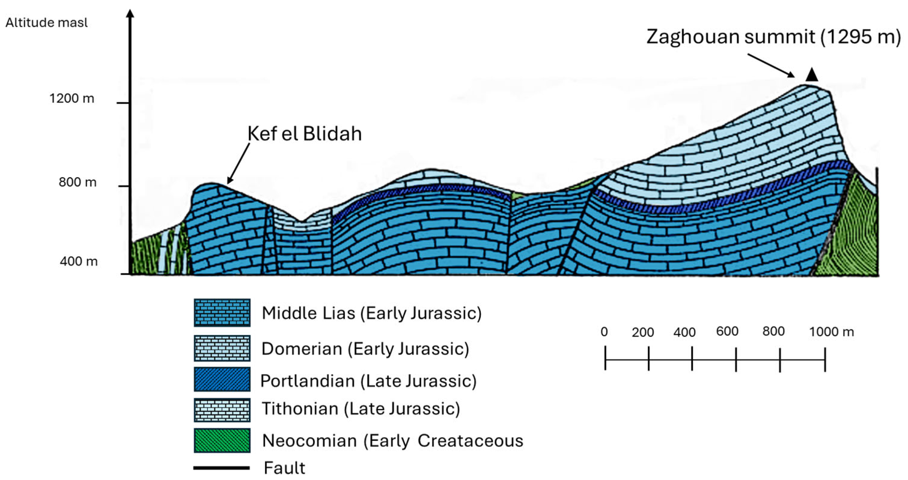
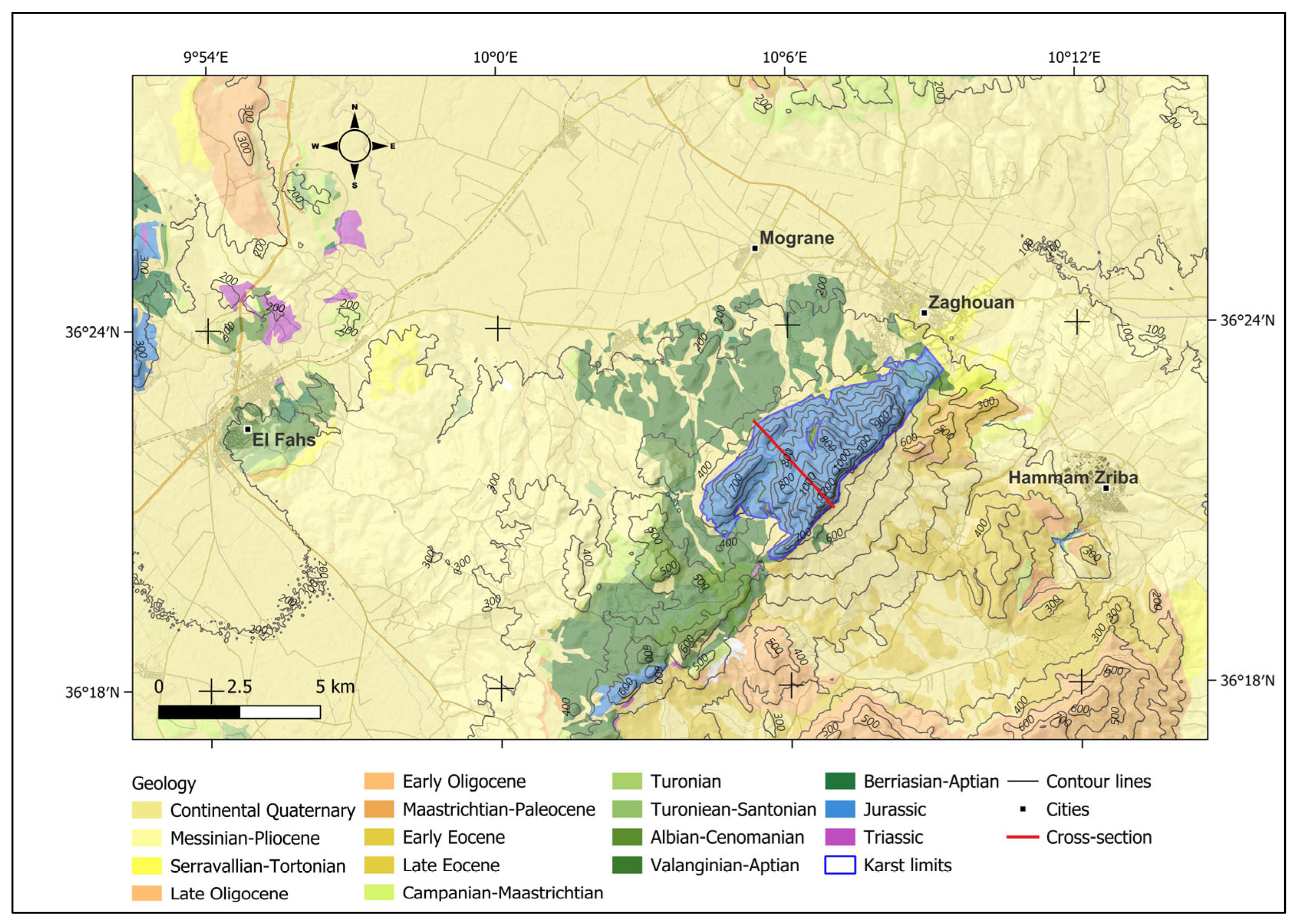
The Zaghouan anticline is primarily composed of Jurassic limestones, bordered by rock-fall deposits and Cretaceous outcrops. As illustrated in Figure 3 and Figure A1, the geology of Jebel Zaghouan is shaped by southern and transverse fault systems, which have segmented the structure into distinct blocks. These faults—namely, Kef El Orma, the Great Peak, and Achilles—facilitate the infiltration of meteoric waters [3]. The eastern part of the Zaghouan karst aquifer provides favorable conditions for groundwater storage [3], whereas the western sector, dominated by marl deposits, exhibits reduced storage capacity [41].
The Jurassic limestone body forms a trapezoidal block, cavernous and highly fractured, extending roughly 8 km along a N–40° E direction and averaging 2.4 km in width along a N–45° W axis. Its surface area covers around 19 km2 at an elevation of 300 m NGT. Surrounded by marl acting as an impermeable barrier, the massif can be divided into three main compartments arranged from north to south:
  • Small Zaghouan, the source of Ain Haroun;
  • The transmission station massifs (Kef El Orma, Kef El Blidah, and Jebel Stâa), the largest compartment, feeding major springs such as the Water Temple (Nymphée), Aïn Ayed, and Aïn Oued El Guelb;
  • The Great Peak massif, which gives rise to the Sidi Medien spring.
The general dip of the limestone strata combined with the northwestern topography accounts for the presence and abundance of springs along the eastern massif and slopes.

2.1.2. Water Resources

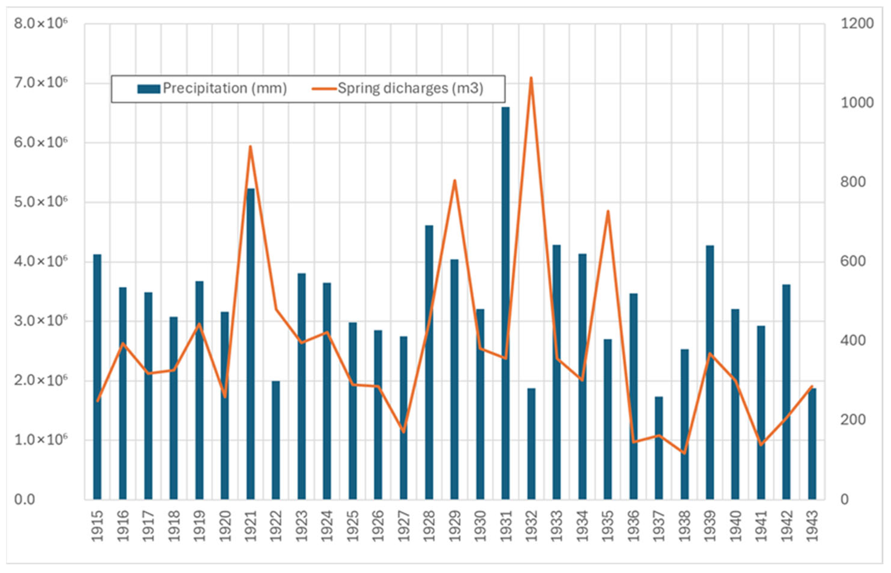
This region experiences an upper semi-arid to sub-humid climate, with variable annual precipitation averaging 467 mm and ranging from 245 to 625 mm over the period 1915–1944. Spatial distribution of rainfall is heterogeneous, and temporal fluctuations are notable (Figure 4). The average annual temperature is around 17.7 °C (https://www.meteo.tn/fr/donnees-climatiques, accessed on 9 October 2020). Historically, the Jebel Zaghouan karst aquifer has been a critical source of drinking water for local cities and the capital, Tunis, previously Carthage during the Roman era [52]. Drinking water was supplied by 132 km of Roman aqueducts, the remains of which can still be seen today along the Tunis Zaghouan Road. The aquifer sustains approximately 14 springs (Ain Essid, Ain Wad el Galb, Ain Ayed, Ain Haroun, Ain Lansarine, Ain Oued Guelb, Galerie 44, Galerie 47, Nila 1, Nymphée, Okka, Sidi Medien, Yahya, and Zkir) (Figure 4) which played a vital role in the local water supply. Additionally, three galleries were constructed to supplement these springs and meet water demand during drought conditions. The first galleries were constructed in 1928 at Ain Ayed. The second one in 1944, followed by the third gallery in 1947. The exploitable reserve of this karst system was quantified at 2.7 million m3 before 1943 (the beginning of the exploitation). During natural functioning, the flow rates exhibited significant variability (Figure 5), ranging from 0.8 to 7 million m3/year.
At present, the Jebel Zaghouan karst aquifer is primarily exploited through a system of nine boreholes and galleries, ensuring the provision of drinking water to the city of Zaghouan and its surrounding rural areas. Among these, three boreholes are dedicated to the abstraction of mineral water for commercial bottling under the brands Cristaline, Aqualine, and Prestine (Figure 4). Since 2015, however, the natural discharge from the galleries has nearly ceased, accompanied by a sustained decline in groundwater levels [53]. In response to the acute water deficit—particularly following the desiccation of Galerie 44 and Galerie 47—two supplementary boreholes, namely Temple and Ain Haroun 3bis, were commissioned in 2017 and 2018 [53].

2.2. Historical Data Collection and Rescue

The input data considered are historical rainfall, temperature, and pressure time series at the daily and weekly scales (Table 2). They were used to model the Zaghouan karst discharge in its natural hydrodynamic functioning.
Historical rainfall, temperature, and pressure data are essential for analyzing long-term trends and variability in our karst system responses. These records, sourced from early 20th-century meteorological service reports and archives of the National Library of Tunisia (Figure A2), address critical gaps in existing datasets. Rescuing and digitizing these data enhances our ability to reconstruct past conditions, refine karst system models, and evaluate changes over time.

2.3. Data Preprocessing

2.3.1. Rainfall

Two historical meteorological stations are located near the Zaghouan karst zone: Zaghouan Contrôle and Zaghouan SM (Figure 4 and Table 3). The primary rainfall dataset analyzed in this study was obtained from the Zaghouan Contrôle station, covering the period from 1915 to 1944.
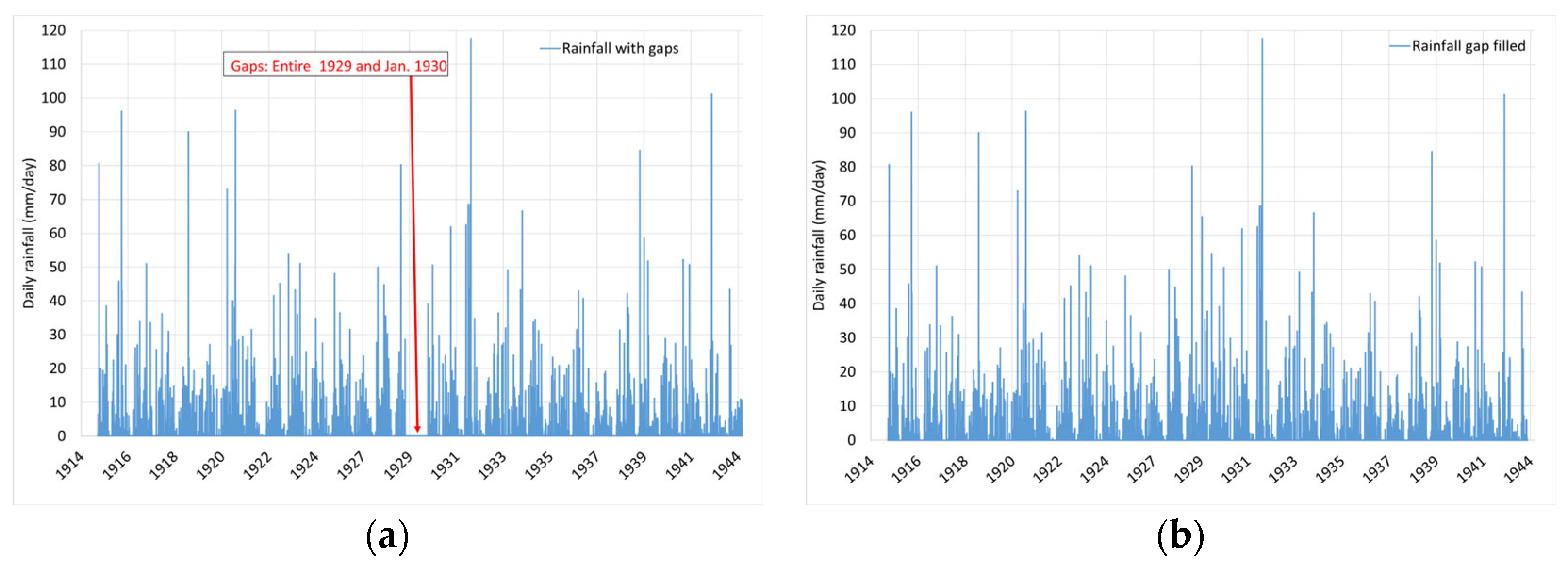
A data gap was identified from 1 January 1929 to 31 January 1930. To address this, linear interpolation was performed using rainfall records from the nearby Zaghouan SM station, situated only a few hundred meters away. This preprocessing step enabled the reconstruction of a continuous daily and weekly rainfall series for the Zaghouan Contrôle station.
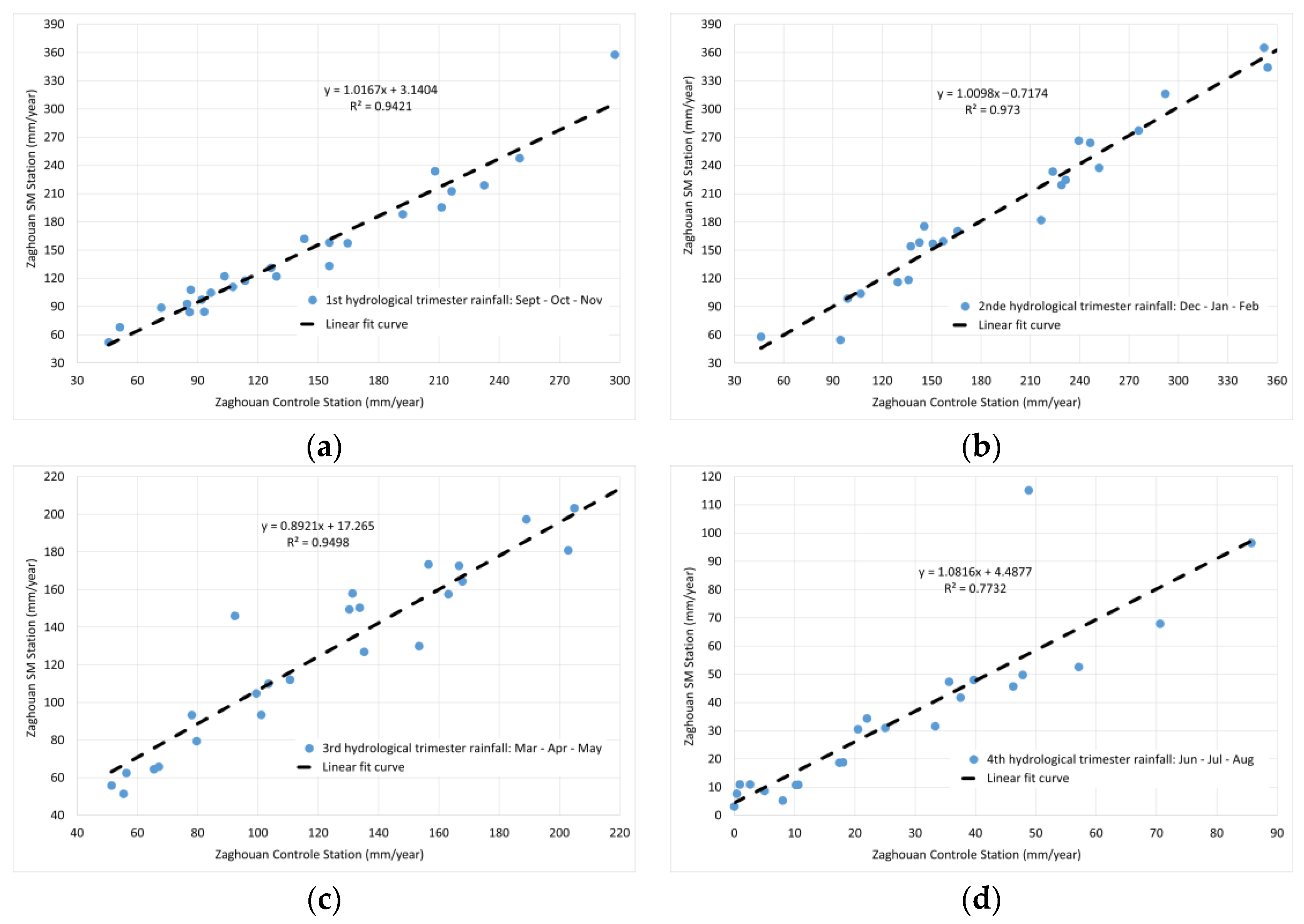
To implement this approach, a correlation analysis was carried out between the annual cumulative rainfall totals of both stations, thereby assessing the reliability of data transposition between the sites. Additionally, the correlation analysis was extended to a trimester basis, according to the hydrological year in Tunisia (starting in September). Rainfall data were divided into four trimesters: September to November (first trimester), December to February (second trimester), March to May (third trimester), and June to August (fourth trimester).
For each trimester, linear regression models were developed using available data. The resulting trimester-specific regression equations were then applied to reconstruct the missing daily rainfall data for the Zaghouan Contrôle station, under the assumption that the quarterly correlations remained valid at the daily scale.

2.3.2. Temperature and Pressure

In addition to rainfall, we use two additional input data types: temperature and pressure, measured on a daily scale. In the karst water balance, temperature and pressure are exogenous variables that influence the quantity of water transitioning from the epikarst to the karst aquifer. Consequently, these variables impact the temporal evolution of discharge at the karst outlet.
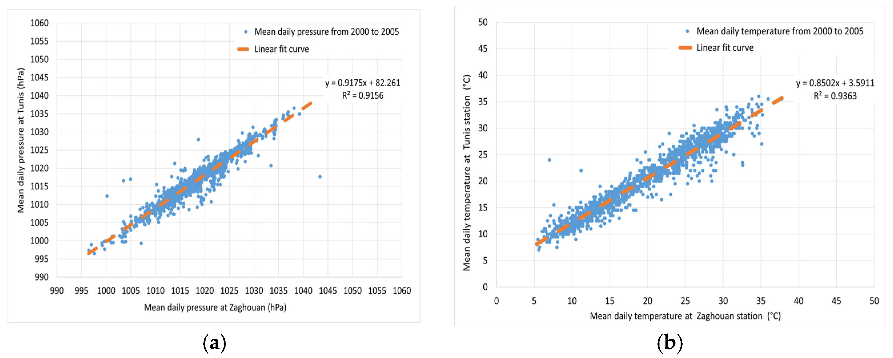
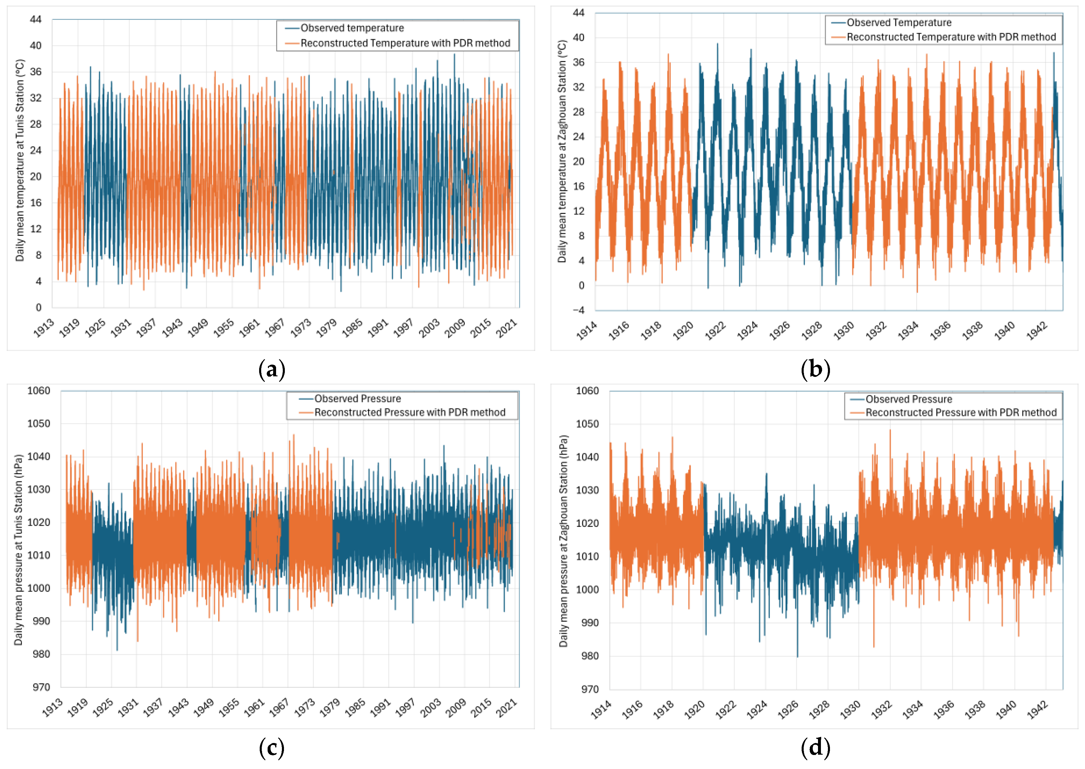
Temperature and pressure data were unavailable at the two study stations during the study period. To address this limitation, we used observations from the Tunis meteorological station, located ~50 km away. Using Tunis as a proxy for Zaghouan is justified because near-surface air temperature and atmospheric pressure exhibit much longer spatial decorrelation scales than precipitation. The climate literature shows that air temperature decorrelates over ~103 km and that pressure/geopotential-height anomalies organize into basin-scale teleconnection patterns, implying high coherence at scales of tens of kilometers [54,55]. This approach is justified by the strong correlation observed between the two locations over a common period from 2000 to 2005 (Figure 6).
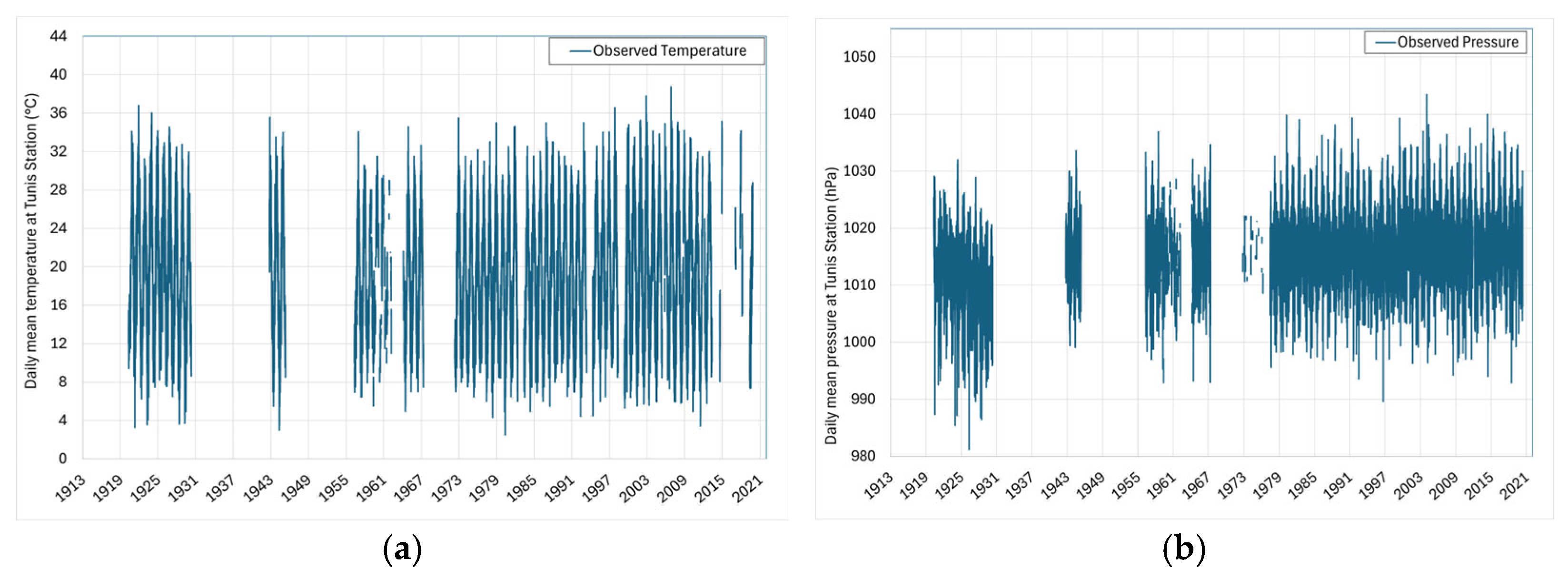
However, Zaghouan station data do not cover the entire study period from 1915 to 1944. Instead, data are available at Tunis station for the period from 1921 to 1930. Unfortunately, this dataset is insufficient to fill the gaps between 1915 and 1921, and between 1931 and 1944 (Figure 7).
To develop a continuous time series, temperature and pressure data from the Tunis meteorological station were compiled for the period 1944–2021, despite the presence of missing values. As data gaps were largely synchronous across both variables, cross-variable imputation was deemed unsuitable. Instead, a reconstruction method was applied to fill the gaps. Following this, temperature and pressure at Tunis were further estimated using linear correlation equations derived from data recorded between 2000 and 2005 at both the Tunis and Zaghouan stations.
Various methods are available for filling gaps in time series data, ranging from simple approaches such as forward/backward filling, mean or median substitution, and linear or spline interpolation, to more advanced techniques including moving averages, regression-based imputation, Kalman filtering, K-Nearest Neighbors (KNN) imputation, Seasonal ARIMA (SARIMA) models, and machine learning methods such as random forests or recurrent neural networks. Ref. [56] suggests that simpler, local methods like interpolation and KNN perform well for short, isolated gaps, but their accuracy declines for long, continuous gaps, where local information is insufficient to capture the underlying dynamics or seasonal patterns. In such cases, Probability Distributions Reconstruction (PDR) offers an effective alternative by reconstructing missing values based on the statistical properties of the observed data, preserving both the probability distribution and seasonal characteristics. PDR models the variable’s distribution rather than relying on neighboring points, generates synthetic values that maintain statistical consistency, and can adapt to temporal and seasonal variations. For extensive gaps, seasonally aware models or the incorporation of external data can also provide more reliable reconstructions. In our study, we used the Probability Distributions Reconstruction (PDR) approach.
Daily values of these variables vary randomly from year to year and across different years for the same calendar day.
Let i represent the number of years (i = 1⋯30) and j the number of calendar days (j = 1⋯365). We define Tij and Pij; as the daily temperature and pressure, respectively, for year i and day j. For each day j, a time series T.j; and P.j; are constructed, yielding 365 series for each variable (730 series). Each series is then fitted with its own probability distribution function, denoted DTj; and DPj;, respectively, resulting in 365 distributions for each variable.
To reconstruct the missing values, a random sample is drawn from a uniform distribution, followed by the calculation of the quantile using, respectively, the inverse of the normal and log normal distribution corresponding to day j.

2.3.3. Discharge at Nymphée Spring

The discharge at the karstic outlet of the Nymphée is a crucial parameter in our modeling efforts. It serves as the output data characterizing the hydrodynamic functioning of the Zaghouan karst system.
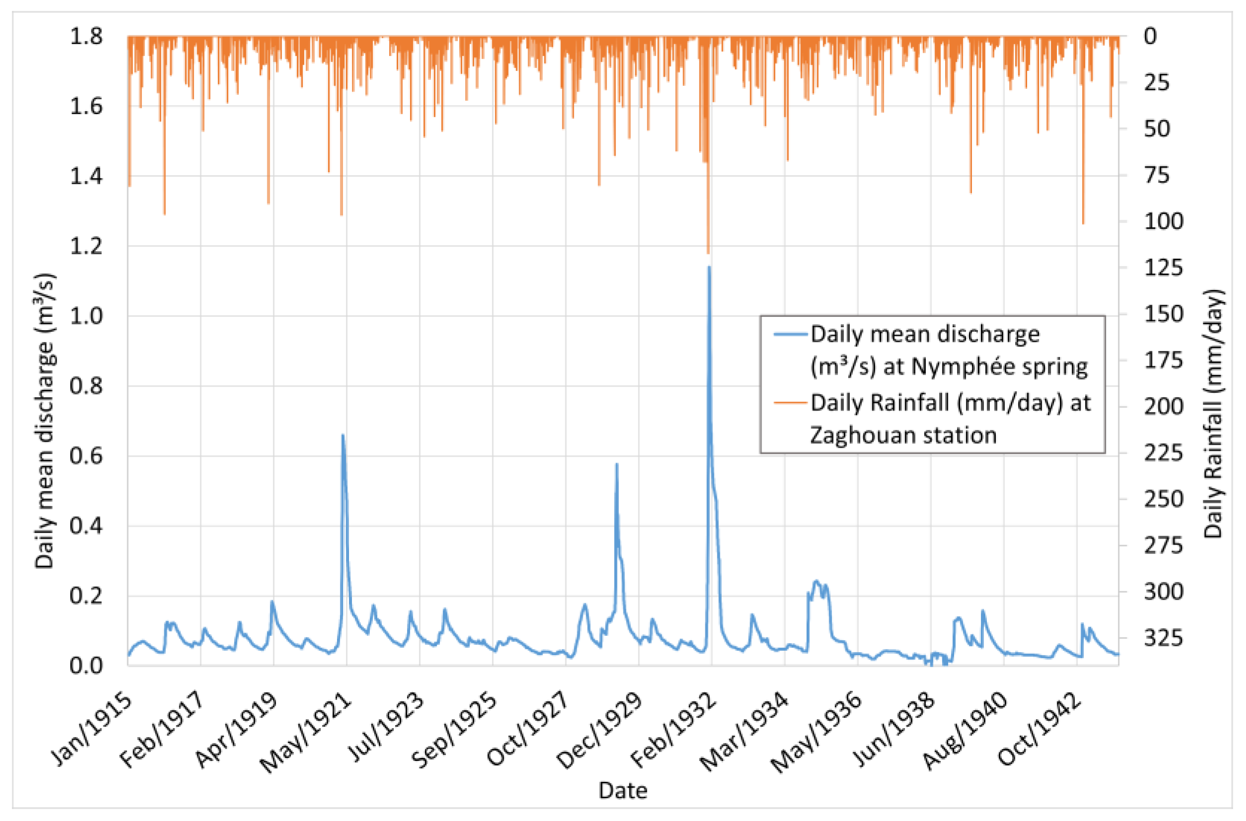
Historical discharge data for the study period from 1915 to 1944 were collected in paper format by SONEDE (DGRE). These discharge records were cataloged using a non-uniform temporal scale, ranging from weekly and biweekly to monthly intervals. The printed records (Figure A3) were scanned and digitized using Optical Character Recognition (OCR) technologies. This digitization process was followed by manual verification and correction to address errors introduced during the conversion. Subsequently, a filtering process was applied to clean the dataset, removing inconsistencies, duplicates, and errors. After the conversion, linear interpolation was performed to obtain a uniform discharge series with a weekly and daily time step (Figure 8). Table 4 shows the main statistical parameters of daily discharges. The highest recorded discharge, approximately 1.140 m3/s (99.99th percentile), occurred on 6 June 1932, following a period of intense rainfall as shown by the concurrent spike in daily precipitation at the Zaghouan station. Similarly, the significant discharge peaks observed on 17 April 1921 (0.65 m3/s; 99.66th percentile) and 23 April 1929 (0.57 m3/s; 99.35th percentile) are closely associated with substantial rainfall events. These findings highlight the piston flow functioning of the karst through its reactivity to extreme rainfall, as illustrated in Figure 8.

2.4. Hydrodynamic Characterization of Karst Through the Discharge at Nymphée

2.4.1. Characterizing Flow Regime Using the Ranked Method

The ranked flow method is used to characterize the flow regime and specific events at the karst outlet through the analysis of its discharge. Proposed by [48], it involves classifying discharge into amplitude classes. Subsequently, a statistical adjustment is applied to the discharge. This adjustment highlights the frequency of exceeding or not exceeding the discharge classes. The representative curve of ranked flows is obtained by plotting the discharge classes on the x-axis and the non-exceedance frequencies on the y-axis [17]. The ranked flow curve facilitates the identification of abnormally high and low flows [34]. Regarding the outlet of the Nymphée of the Zaghouan karst, we determined the ranked discharge curves on a daily scale. This was performed to provide an analysis, visualize, and compare the discharge distribution at different scales. Furthermore, we adopted class amplitudes proportional to the sample size of each time scale (N), with the amplitude A calculated as follows: A = √N.

2.4.2. Estimating Memory Effect Using Autocorrelation of Discharge

The autocorrelation of the discharge variable (Equations (1) and (2)), also referred to as serial correlation, measures the linear correlation of the discharge with itself at different time lags k:
r k = C k σ x 2
C k = 1 n i = 1 n k x i x ¯ x i + k x ¯
where r k the autocorrelation coefficient at lag k. It measures the linear relationship between the time series and its lagged version, C k   the covariance between the time series xi and its lagged version x i + k . Here, n is the sample size, corresponding to the temporal lag (in days, weeks, or months); x represents the discharge at time t, x ¯ is the mean discharge of the series, and σx denotes the standard deviation [11].
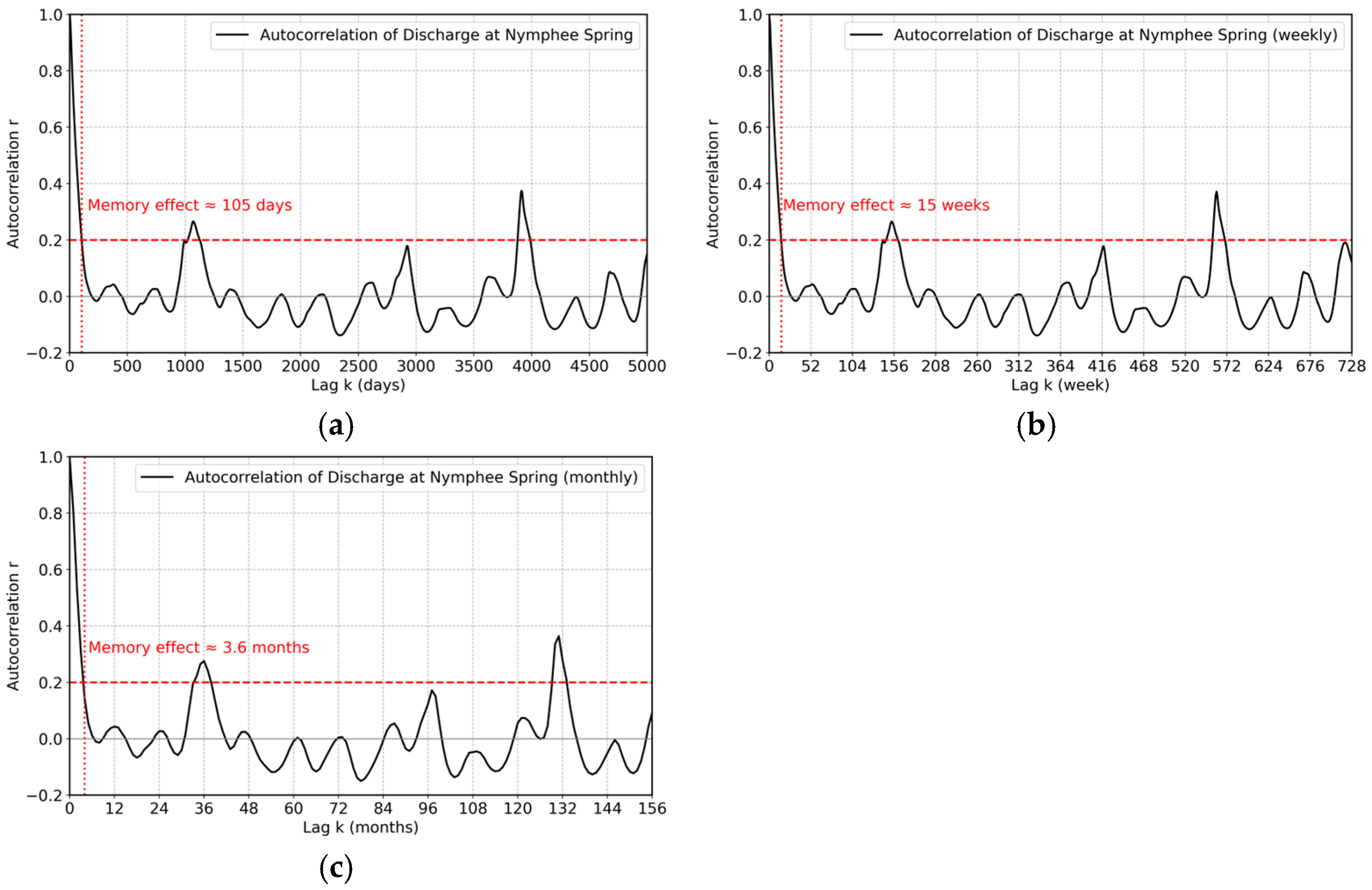
The autocorrelation structure of Nymphée spring is analyzed through the autocorrelation function (ACF), which plots autocorrelation coefficients against the corresponding lag times. It enables the characterization of the system’s memory effect, defined as the lag necessary for the autocorrelation coefficient to reach a minimal threshold, commonly set at 0.2 [57]. This memory effect represents the maximum duration during which the discharge significantly correlates with itself, indicating the inertia of the karst system [17,34]. For the Nymphée spring at Zaghouan, we computed and analyzed autocorrelograms based on daily (Figure 9a), weekly (Figure 9b), and monthly (Figure 9c) discharge data. Then, the memory can be summarized depending on the temporal scale in Table 5.
The ACFs of the three discharge time scales at Nymphée Spring exhibit a rapid decline over the first lags, followed by oscillations around zero after approximately 105 days, 15 weeks, and 3.6 months, respectively. This pattern reflects a finite memory effect of the aquifer system rather than a persistent long-term trend. If a deterministic trend were present, the ACF would decay more gradually and remain positive over long lags; since this behavior is not observed, detrending was not applied. Although an exponential model with a sill equal to 1 can be appropriate for correlation structures characterized by monotonic decay, the observed ACF displays oscillatory dynamics associated with recharge and release processes. Consequently, interpreting the characteristic memory time provides a more meaningful representation of aquifer behavior, as it captures the underlying hydrogeological processes.

2.4.3. Estimating Lag Time Using Cross Correlation and Significance Test Between Rainfall and Discharge

  • Cross correlation
In addition to the autocorrelation analysis discussed previously, the cross-correlation (Equations (3) and (4)) between precipitation and discharge time series offers valuable insight into the transfer dynamics of the karst system. The cross-correlation coefficient (rk) is used to quantify the relationship between the two series as a function of the temporal lag k (in days, weeks, or months), and is defined as follows:
r k = C k σ x σ y
C k = 1 n i = 1 n k x i x ¯ y i + k y ¯
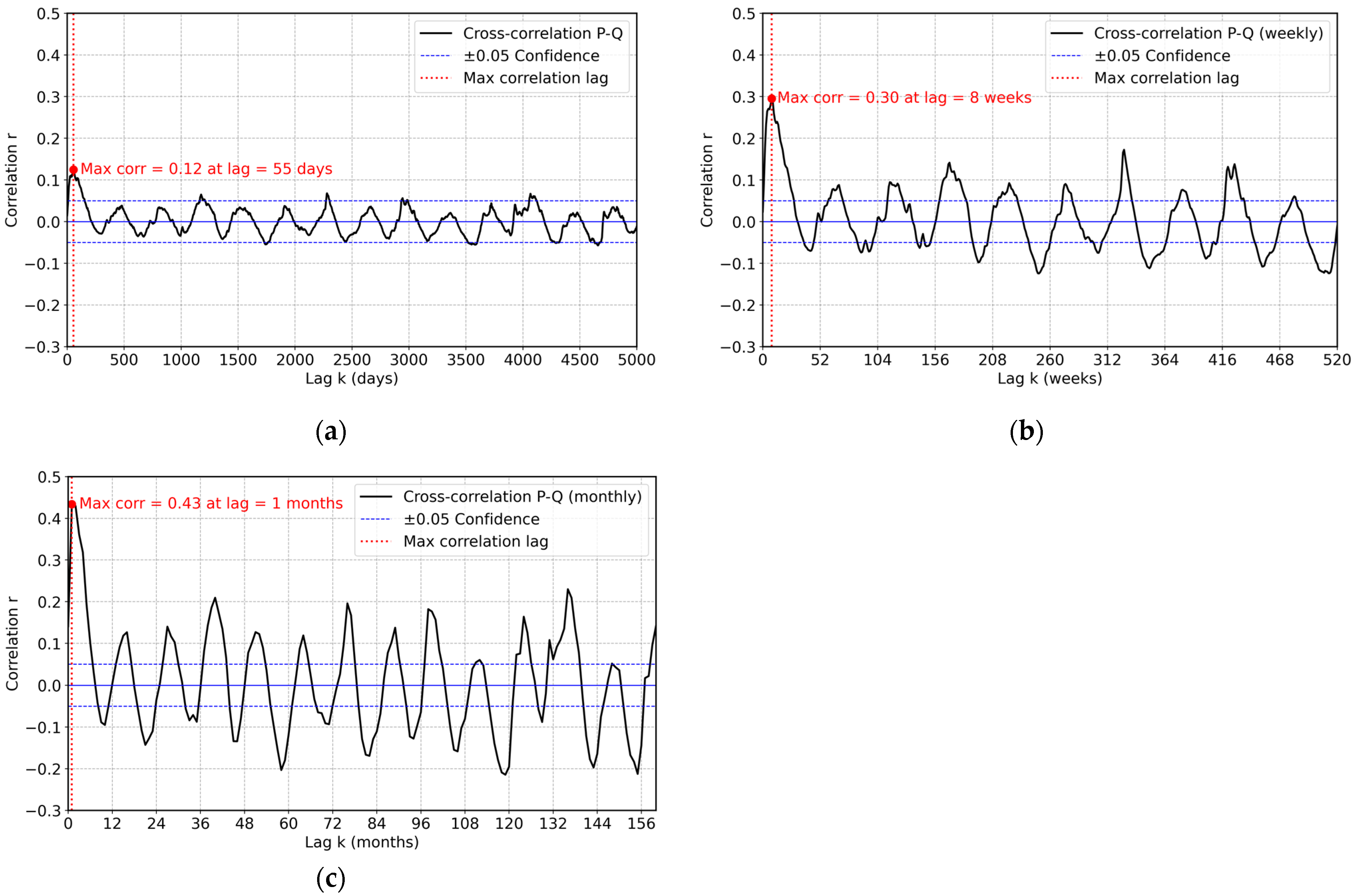
where n is the sample size; k is the time lag (in days, weeks, or months); x i represents rainfall; x ¯ is the mean of the rainfall series; σ x is the standard deviation of the rainfall sample; y i + k represents discharge; y ¯ is the mean of the discharge series; and σ y is the standard deviation of the discharge sample. The cross-correlogram produced from this analysis characterizes the temporal relationship between rainfall and discharge, identifying the lag period that reflects the response time of the aquifer to precipitation events. In a causally linked system, a positive lag indicates the period during which rainfall exerts a direct influence on discharge. This lag is governed by the internal functioning of the aquifer, and its extent—the so-called memory effect—represents the maximum duration over which rainfall continues to affect discharge [58]. In this study, cross-correlograms were generated for daily, weekly, and monthly discharge series (Figure 10a–c), allowing for the determination of characteristic response times and a comprehensive assessment of the persistence of rainfall’s influence on the karst system’s hydrodynamics. The correlograms show a high degree of variability around zero. This “noisy” character is mainly due to the irregularity of rainfall events and the reduction in the number of effective observations in the semi-arid context. Nevertheless, interpretation is not based on point-to-point fluctuations, but on the location of the significant maximum. Here, the maximum correlation reflects the characteristic response time of the karst system.
Table 6 presents the lag times at which precipitation (P) and discharge (Q) series show their strongest linear correlation at daily, weekly, and monthly temporal scales. These values emphasize the linear temporal link between P and Q, while acknowledging that other factors also influence the hydrodynamics of the karst system.
  • Significance testing
To deepen the characterization of the dependence between the rainfall and discharge time series, we applied a significance test using Kendall’s rank correlation coefficient τ in different temporal scales (Equation (5)):
τ > u α / 2 · 2 2 n + 5 9 n n 1
where n is the sample size, α is the significance level, and uα/2 is the α/2 percentile of the Normal distribution (uα/2 = 1.96).
No significant instantaneous dependence was found between rainfall and discharge at daily, weekly, or monthly scales, which is consistent with the delayed hydrodynamic response typical of karst systems. To further assess the karst’s response time, we conducted additional significance tests using lagged discharge series relative to rainfall. This approach enabled us to identify the lag at which Kendall’s τ reaches its maximum value (Table 7). The results reveal a substantial increase in correlation when the appropriate lag is applied: at the daily scale, a lag of 114 days produced a significant τ; optimal lags of 18 weeks and 3–4 months were found for the weekly and monthly scales, respectively. On average, the optimal lag across all temporal scales is about 115 days, which corresponds to the characteristic response time of the system. Kendall’s τ and cross-correlation address complementary aspects of the rainfall–discharge relationship. Kendall’s τ, being a non-parametric rank-based test, evaluates the statistical significance of monotonic dependence and helps identify the characteristic lag. Cross-correlation, in contrast, quantifies the linear dependence as a function of lag, providing insight into the dynamic transfer of signals. By combining both approaches, we capture both the statistical significance of monotonic dependence (Kendall’s τ) and the temporal dynamics of linear dependence (cross-correlation), which together offer a more robust characterization of the karst aquifer response. The results show that cross-correlation analysis highlights shorter response times (55–56 days at daily and weekly scales, and 30 days at the monthly scale), reflecting the influence of rapid flow components. In contrast, Kendall’s τ identifies longer lags of about 115–126 days, which represent the dominant delayed response of the aquifer. This duality is consistent with the hydrodynamic behavior of karst systems, where both quick conduit drainage and slow diffuse flow coexist, the latter controlling the overall system inertia. The pronounced lag, therefore, further supports the conclusion that the Zaghouan karst is characterized by low hydraulic inertia and a slow response to rainfall inputs. Consequently, the hydrodynamic characterization is identified as a C6-type aquifer under the typology of [27,50,53] with moderate variability and delayed discharge response.

2.5. ANN Modeling Approaches

In this study, we simulate Zaghouan karst Nymphée spring discharge with deep learning models: MLP, CNN, and LSTM. The approach used meteorological (rainfall, temperature, and pressure) data as input and the discharge as output. The details of each modeling approach can be found in Appendix B.

2.5.1. Models Architectures

  • MLP
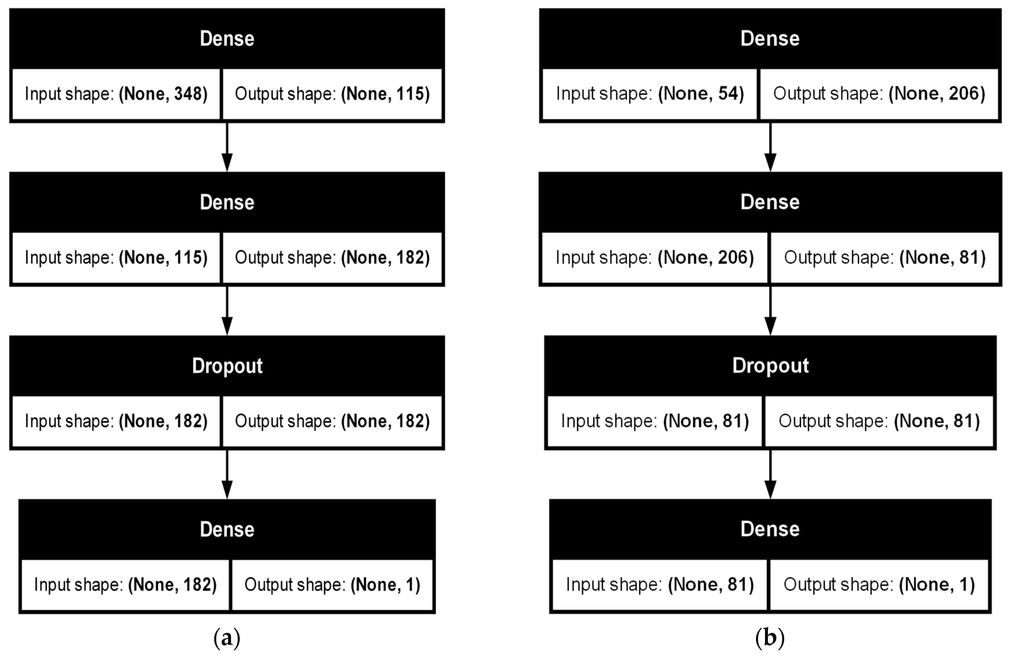
Our MLP models for daily and weekly forecasting have been structured to capture complex, nonlinear relationships between inputs and karst aquifer discharge. Both architectures include dense layers interspersed with dropout layers to prevent overfitting and enhance generalization (Figure 11):
MLP model for daily forecasting consists of an input layer with 348 neurons, connected to a first dense layer of 115 neurons activated by ReLU. A second dense layer expands this representation to 182 neurons, again activated by ReLU. After this, a dropout layer (rate determined by Bayesian optimization) is included to mitigate overfitting. Finally, the output is generated through a dense layer with a single neuron, providing the predicted discharge value.
MLP model for weekly forecasting starts with an input layer of 54 neurons feeding into a dense layer of 206 neurons with ReLU activation. A subsequent dense layer reduces dimensionality to 81 neurons. Similarly to the daily model, a dropout layer is applied here for regularization. The output layer is again a dense layer with one neuron, yielding the weekly discharge forecast.
  • CNN
Our CNN architectures are structured to capture local patterns and temporal features effectively:
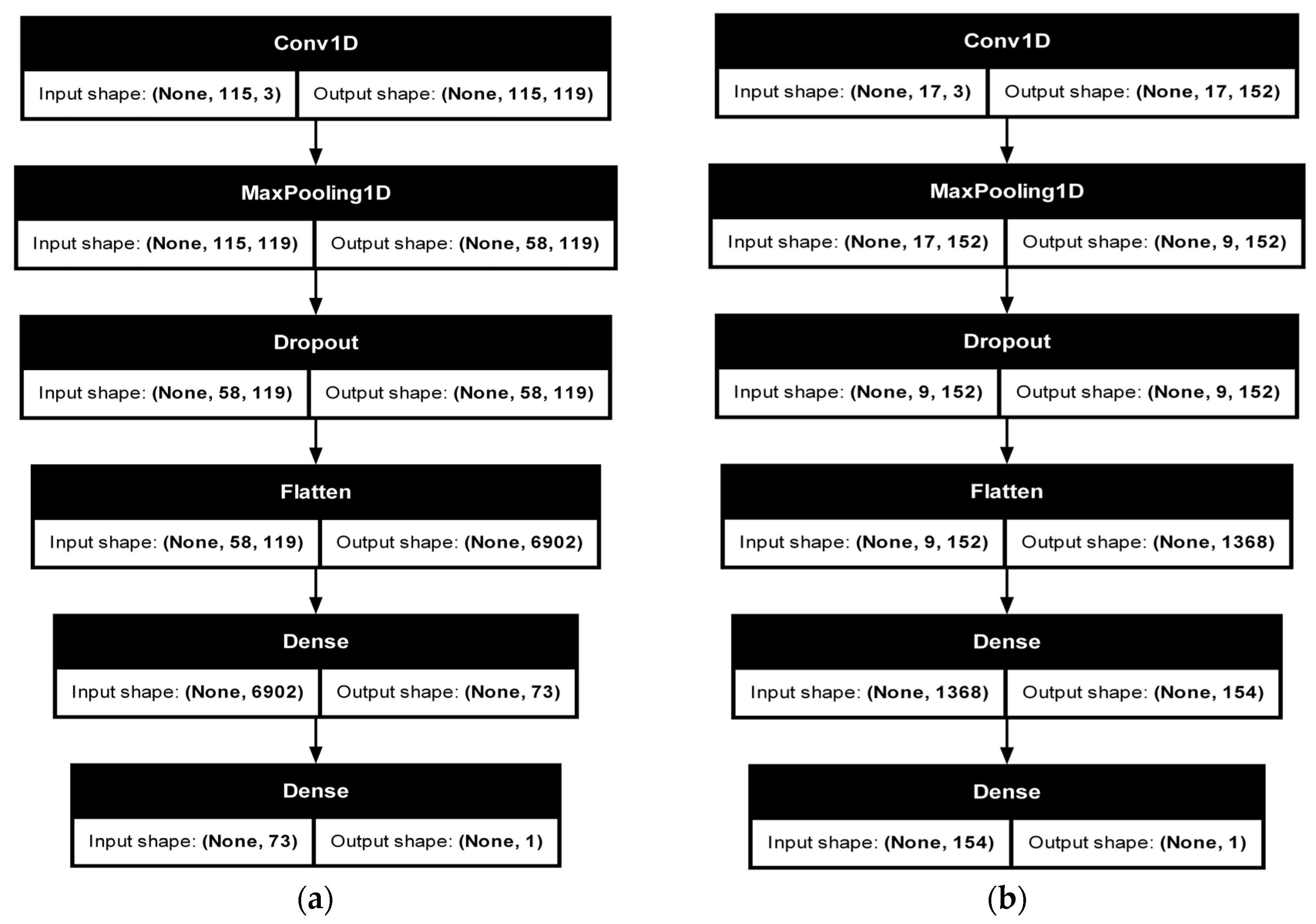
CNN model for daily forecasting consists of an initial 1D convolutional layer (Conv1D) with 119 filters and a kernel size of 3, followed by a MaxPooling1D layer to reduce temporal dimensionality. Subsequently, a dropout layer is introduced to mitigate overfitting. The output from dropout is flattened and passed through a dense layer comprising 73 neurons (activated with ReLU), followed by a final dense layer with a single neuron outputting the forecast discharge.
CNN model for weekly forecasting follows a similar but adjusted structure, starting with a Conv1D layer featuring 152 filters (kernel size of 3). A subsequent MaxPooling1D layer reduces feature size, followed by dropout. The flattened output is then processed through a dense layer containing 154 neurons with ReLU activation. Lastly, a dense output layer with a single neuron provides the predicted weekly discharge (Figure 12).
  • LSTM
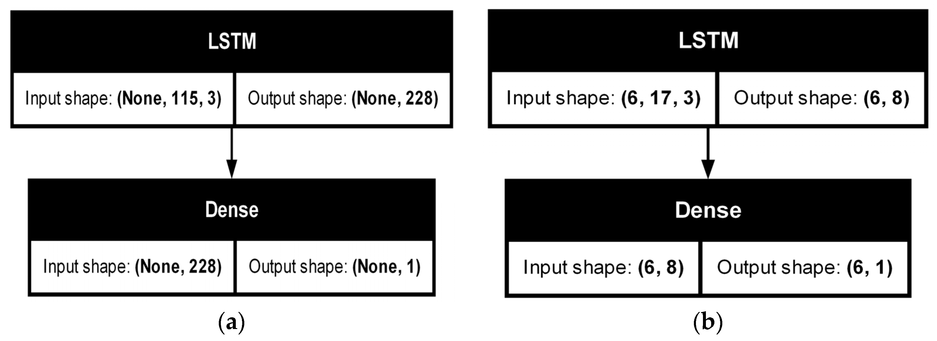
Our LSTM architectures are specifically designed to model long-term temporal dependencies within the discharge time series (Figure 13):
Daily forecasting model begins with an LSTM layer that accepts input sequences of shape (115, 3), producing an output sequence of 58 time steps, each with 128 features. A Dropout layer is subsequently applied to reduce the risk of overfitting. The resulting sequence is then flattened and processed by a dense layer comprising 73 units with ReLU activation. Finally, a single-unit dense layer provides the predicted daily discharge.
weekly forecasting model employs a similar structure, initiating with an LSTM layer that processes input sequences of shape (17, 3) and outputs a sequence of 9-time steps with 128 features each. Following dropout regularization, the output is flattened and passed through a dense layer containing 154 ReLU-activated units, culminating in a single-unit dense layer that generates the weekly discharge prediction.

2.5.2. Hyperparameter Tuning and Evaluation

For all three architectures, we applied Bayesian Optimization to tune hyperparameters (Table 8). We were inspired by the Python 3.13.5 implementation performed by [59]. We used 50 optimization steps with 10 repetitions per step. We also adopt stops if no improvement after 10 consecutive steps.
Also, in all three models, the acquisition function used is expected improvement, while the optimization target function is defined as the mean of the Nash–Sutcliffe efficiency (NSE, Equation (6)), the squared Pearson’s correlation coefficient (R2, Equation (7)) and the Kling Gupta coefficient (KGE, Equation (8)). These three criteria are widely recognized and well established for evaluating forecast accuracy, particularly in water related studies [60]. Their combined use ensures a comprehensive assessment of model performance, capturing both the predictive accuracy and the strength of linear relationships in the forecast outputs.
NSE = 1 i = 1 n x i obs x i pred 2 i = 1 n x i obs x ¯ obs 2
R 2 = 1 i = 1 n x i obs x i pred 2 i = 1 n x i obs x ¯ obs 2
KGE = 1 r 1 2 + α 1 2 + β 1 2
where
  • x i obs observed value at time step i;
  • x i pred simulated value at time step i;
  • x ¯ obs : Mean of observed values
  • r: Pearson correlation coefficient between observed and simulated values
  • α: Variability ratio (standard deviation ratio)
  • β: Bias ratio (mean ratio)
All three model types in this study were trained with a maximum of 150 epochs. To mitigate overfitting, early stopping with a patience of 10 epochs was implemented. The testing period for model evaluation spanned from 1915 to 1921, during which the data were exclusively used for testing purposes. So, the full dataset going from 1915 to 1944 were divided into three subsets: 80% for training, 10% for early stopping, and 10% for validation during hyperparameter optimization.
To ensure consistency, all data were normalized between −1 and 1, and models were initialized randomly based on the random seed. To account for this dependency, each optimization step was repeated ten times, with the mean target function value recorded. We adopt a sequence-to-value (seq2val) set up: given a fixed-length window of past inputs, the model predicts the next time-step discharge. We chose seq2val because our objective is one-step-ahead forecasting at daily and weekly scales; unlike seq2seq, it avoids compounding multi-step errors, simplifies training and tuning, and maximizes data use via sliding windows. In fact, for modeling the discharge at date t, we used input data: rainfall, temperature and pressure at time t − Xi where Xi is the modeling shift time (Equation (9)).
Q ^ t = f X t X i = f R t X i ,   T t X i , P t X i
where
  • Q ^ t : Predicted discharge at time t
  • f: Model function trained to map inputs to discharge
  • X t X i : Input feature vector at time t − Xi
  • R t X i : Rainfall at time t − Xi
  • T t X i : Temperature at time t − Xi
  • P t X i : Pressure at time t − Xi
  • Xi: Time shift (lag) used in the sequence

2.5.3. Data Splitting Strategy

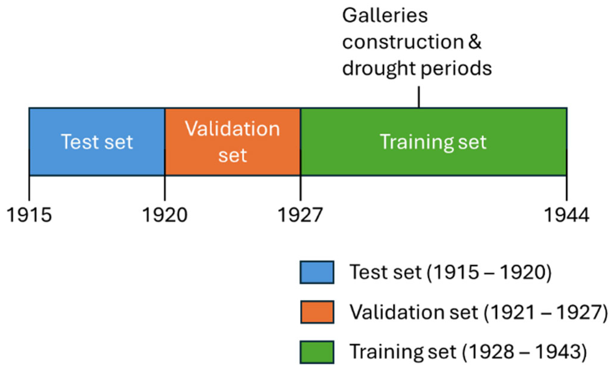
To ensure robust and unbiased evaluation of the ANN models, our historical dataset (1915–1944) was chronologically divided into three subsets (Figure A4), reflecting specific hydrological contexts and historical developments within the Jebel Zaghouan karst system:
  • Test set (1915–1920, ~10%): This initial period, untouched by model training, was exclusively used to evaluate model predictive capabilities on completely unseen data.
  • Validation set (1921–1927, ~10%): Immediately following the test period, this set was utilized for early stopping and hyperparameter tuning to prevent overfitting.
  • Training set (1928–1944, ~80%): The most recent period, encompassing significant events including drought episodes and the construction of galleries in 1928 and 1944, was reserved for training the neural networks. This period was selected deliberately to capture the aquifer’s hydrodynamic responses under specific varying stresses.
This chronological data-splitting approach preserves temporal dependencies inherent in hydrological systems and reflects real-world forecasting conditions, thus enhancing the models’ operational applicability.

3. Results

3.1. Data Pre-Processing

3.1.1. Rainfall

The main statistical characteristics of the Zaghouan Contrôle and Zaghouan SM stations are summarized in Table A1. In the data collected, there are some gaps reported. In order to fill them, a linear correlation analysis on an annual scale was performed and showed a strong correlation (R2 = 0.97) between the two stations (Figure 14).
To capture potential seasonal variability in the correlation, linear regression was also performed for each hydrological trimester. The resulting models showed strong consistency, justifying their use in filling daily gaps (Figure 15):
The trimester-wise correction method enabled the reconstruction of a complete daily rainfall dataset for the period 1915–1944, allowing to fill gaps and obtain continuous daily data for the entire study period (Figure 16).

3.1.2. Temperature and Pressure

Daily mean temperature and pressure values for the Tunis station were reconstructed using the PDR approach. The agreement between reconstructed and observed data was evaluated over the full overlapping period (2000–2005). The results show an RMSE of 3.7 °C with R2 = 0.97 for temperature, and an RMSE of 8.4 hPa with R2 = 0.99 for pressure. Based on the established correlations, these parameters were then estimated at the Zaghouan karst site for the period 1915 to 1944 (Figure 17).

3.1.3. Discharge

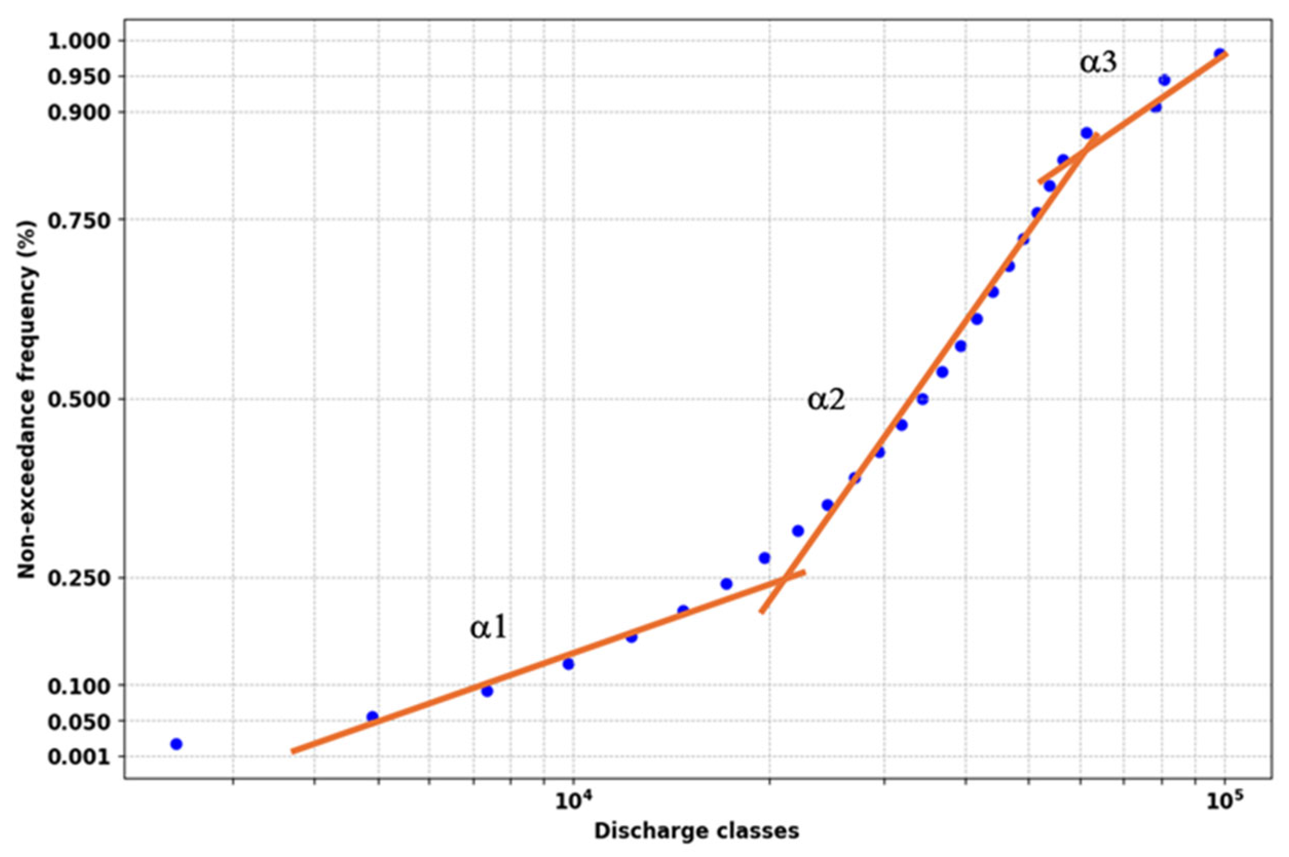
A class interval of 0.011 m3/s (950 m3/day) was defined for flow ranking, resulting in 102 hb. The ranked flow series was then fitted with a log-normal distribution to construct the flow duration curve (Figure 18). Slope breaks, marked by red lines, correspond to operational discontinuities in the karst system and are interpreted in Table A2. The presence of a double inflection indicates reservoir effects—specifically, water storage during recession and delayed release during low-flow conditions. These features are characteristic of poorly drained karst systems, either due to limited karstification and fracturing of carbonate aquifers or boundary-controlled drainage, which reduces the system’s responsiveness to rainfall. In such contexts, the karst acts as a filter, attenuating rainfall signals.
The obtained flow regime was classified as type E, in line with [61], who notes that in poorly drained or boundary-controlled karst systems, the transmission of rainfall variability is significantly dampened.

3.2. Hyperparameters

The Bayesian optimization, conducted for each ANN architecture with 50 steps with 10 repetitions per step can be evaluated with the best iteration and its best corresponding target (Table 9).
The best combination of optimized hyperparameters for each ANN architecture across daily and weekly temporal scales is summarized in Table 10. The optimized hyperparameters include input sequence length, batch size, dropout rate, and learning rate.
The optimal hyperparameters obtained from Bayesian optimization show distinctions among models and temporal scales, highlighting their different sensitivities to the karst system’s hydrodynamic complexity. Sequence lengths (115–126 days) emphasize the significant temporal dependencies inherent to karst hydrology. CNN models require larger batch sizes and higher dropout rates, indicating greater complexity and stronger regularization needs, whereas LSTM models prefer smaller batches and lower learning rates, reflecting their capacity to precisely capture sequential dependencies. MLP maintains moderate values, balancing computational efficiency and stability. These differences underscore the necessity of tailored hyperparameter tuning to optimize each model’s predictive performance for karst aquifer modeling.

3.3. Performance by Model and Temporal Scale

The methodology was focused on 3 ANN architectures: MLP, CNN, and LSTM. All of them were analyzed on a daily and weekly temporal scale to model discharge based on climatic input variables: rainfall, temperature, and pressure.

3.3.1. MLP

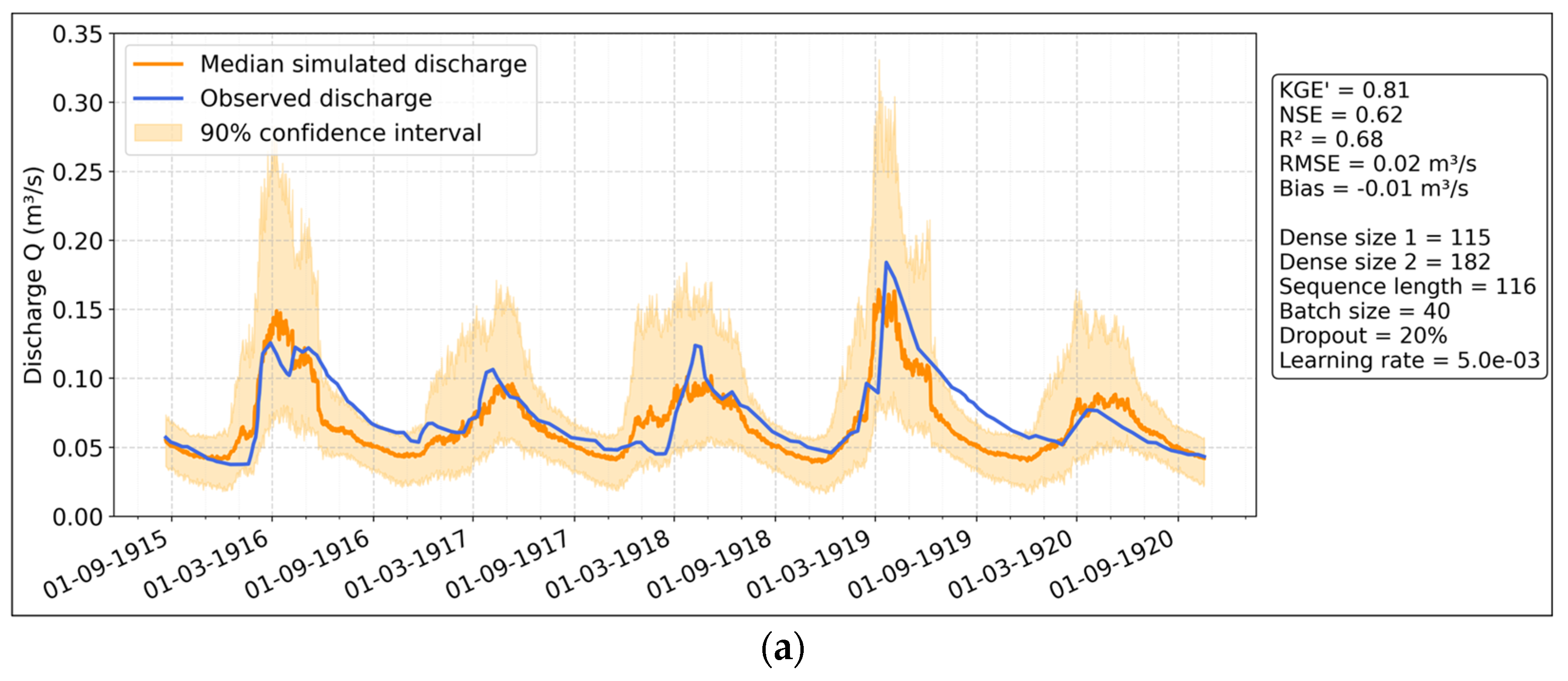
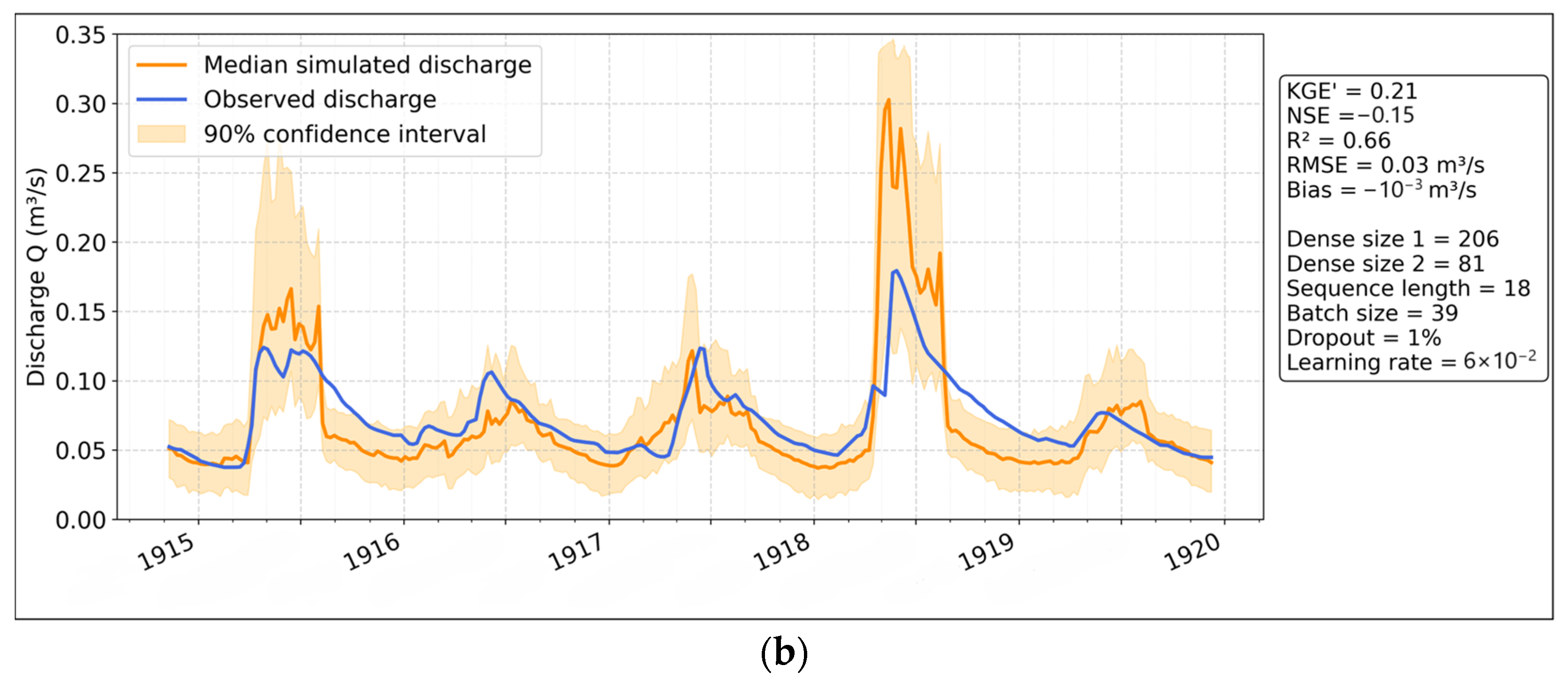
The MLP model at the daily scale (Figure 19a) performs well, with KGE’ = 0.81, NSE = 0.62, and R2 = 0.68, indicating strong predictive capability. The confidence interval is narrow, reflecting stable predictions. However, the model overestimates discharge by 55.41% on average, while underestimation is minimal at 0.27%. At the weekly scale (Figure 19b), the model’s performance drops significantly (KGE’ = 0.21, NSE = −0.15, R2 = 0.66). The widening confidence interval suggests greater uncertainty, and overestimation remains high, further emphasizing the model’s inability to generalize effectively over longer periods.

3.3.2. CNN

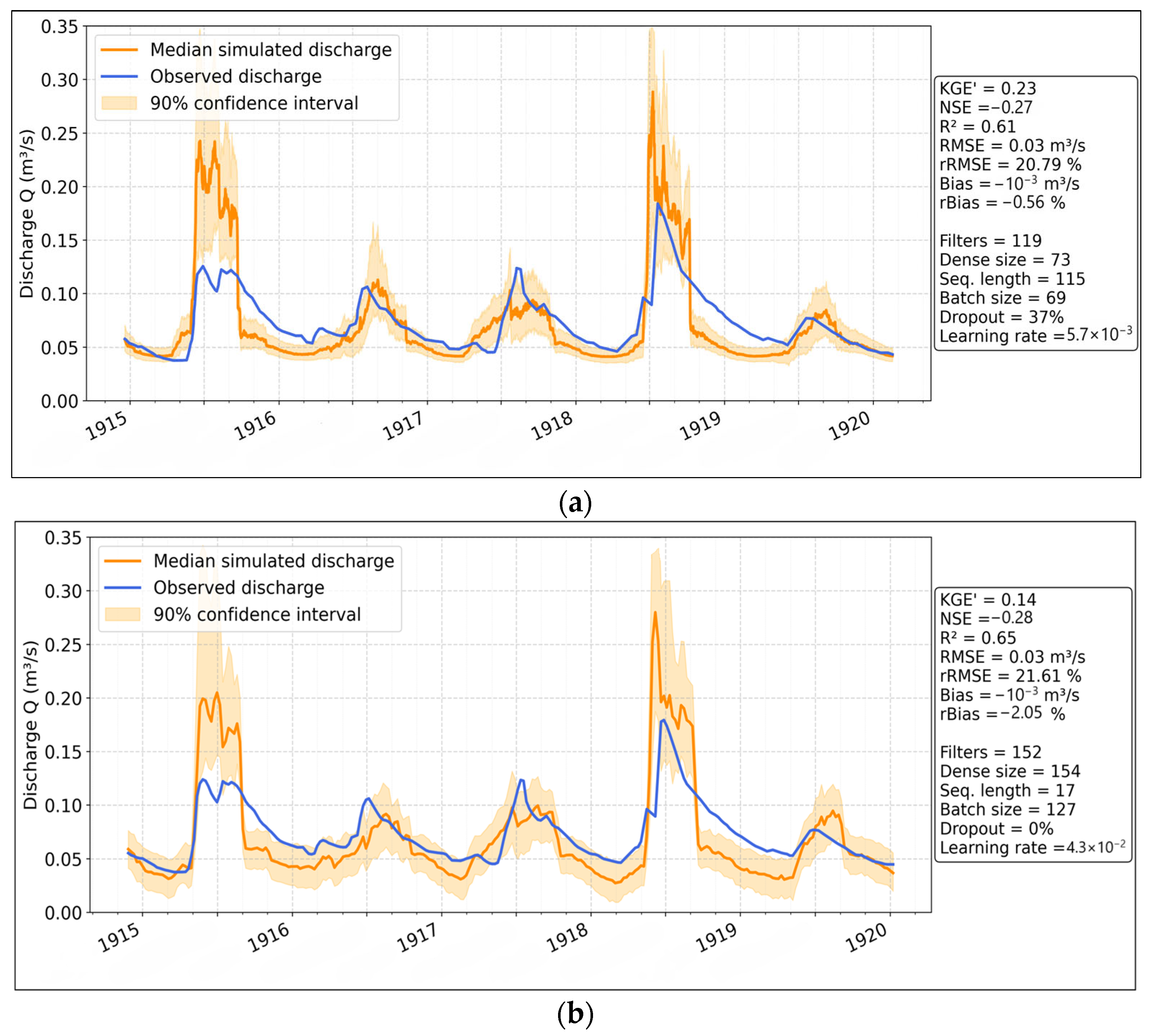
The CNN model at the daily scale struggles (Figure 20a), showing weak correlation (KGE’ = 0.23, NSE = −0.27, R2 = 0.61). The predicted discharge deviates substantially from observations, with overestimation exceeding 55%, and wide confidence intervals reflecting high uncertainty. Underestimation is negligible. At the weekly scale (Figure 20b), the model further deteriorates (KGE’ = 0.14, NSE = −0.28, R2 = 0.65). It fails to capture peak discharge events accurately, and the confidence interval remains wide, confirming its lack of reliability. Overestimation continues to dominate, reinforcing that CNN is not well-suited for this forecasting task.

3.3.3. LSTM

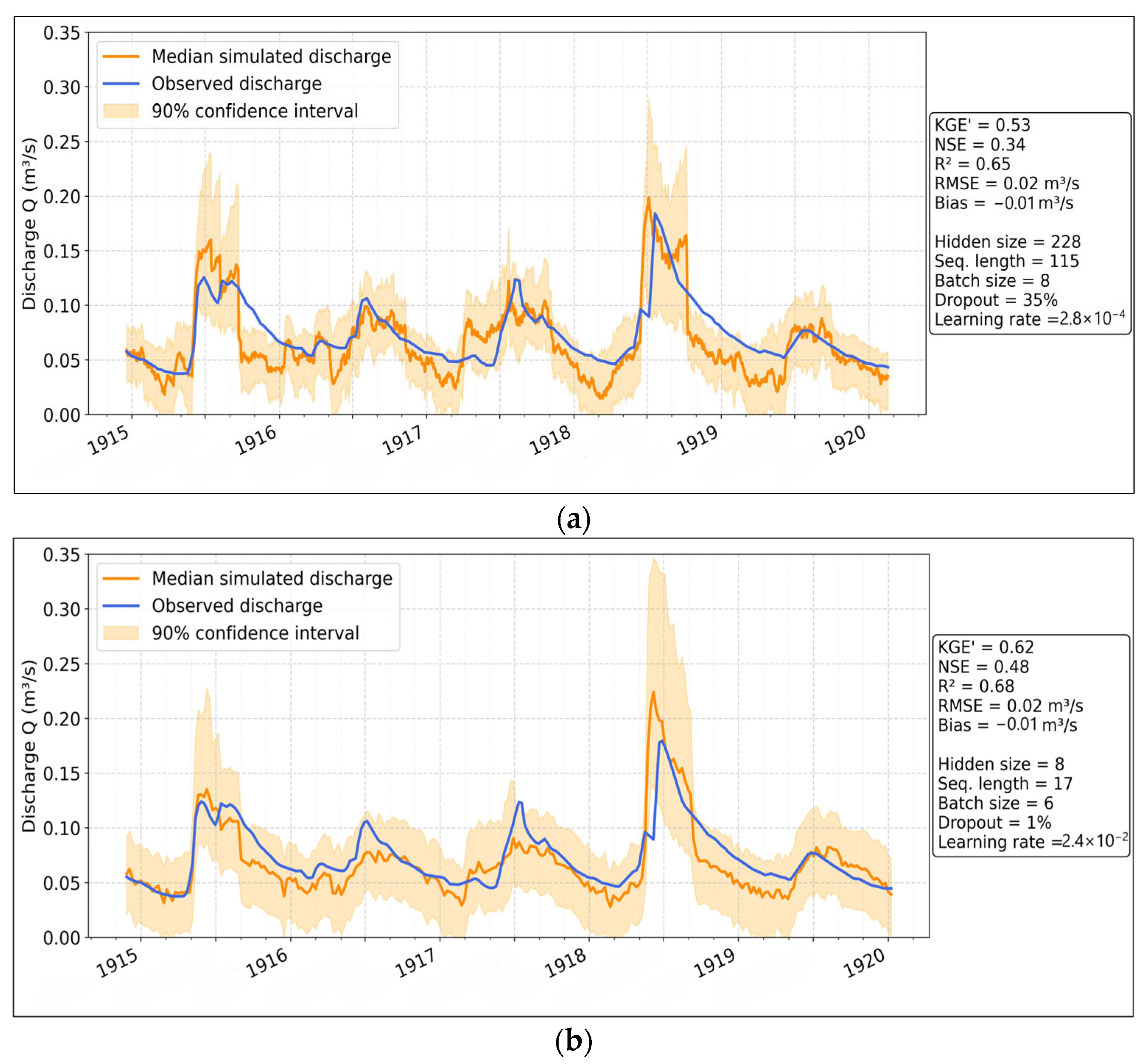
The LSTM model at the daily scale (Figure 21a) performs moderately well (KGE’ = 0.53, NSE = 0.35, R2 = 0.65), with reasonable trend following capabilities but some deviation in peak discharge predictions. Overestimation is present but generally lower than that of CNN and MLP. Underestimation remains minimal. At the weekly scale (Figure 21b), the model significantly improves (KGE’ = 0.62, NSE = 0.48, R2 = 0.68), making it the most reliable option for long-term forecasting. The confidence interval is narrower compared to the other models, indicating higher prediction stability. Overestimation is still present but less pronounced than in MLP and CNN, making LSTM the best-suited model for long-term predictions.

3.3.4. Overall Performance

This analysis evaluates the predictive performance of the three ANN architectures (MLP, CNN, and LSTM) at daily and weekly temporal scales using KGE’, NSE, and R2 metrics (Table 11). The MLP model provides the highest accuracy at the daily scale (KGE’ = 0.81, NSE = 0.62, R2 = 0.68) but significantly deteriorates for weekly forecasts. CNN consistently underperforms at both scales, with low KGE’ (≤0.23) and negative NSE values, reflecting substantial deviations from observed discharges. Conversely, the LSTM model exhibits moderate daily performance and demonstrates superior reliability at the weekly scale (KGE’ = 0.62, NSE = 0.48, R2 = 0.68). Additionally, MLP and CNN show significant prediction bias (maximal global overestimation > 55%), whereas LSTM maintains more stable predictions, emphasizing its ability to capture the hydrological response effectively over longer periods.
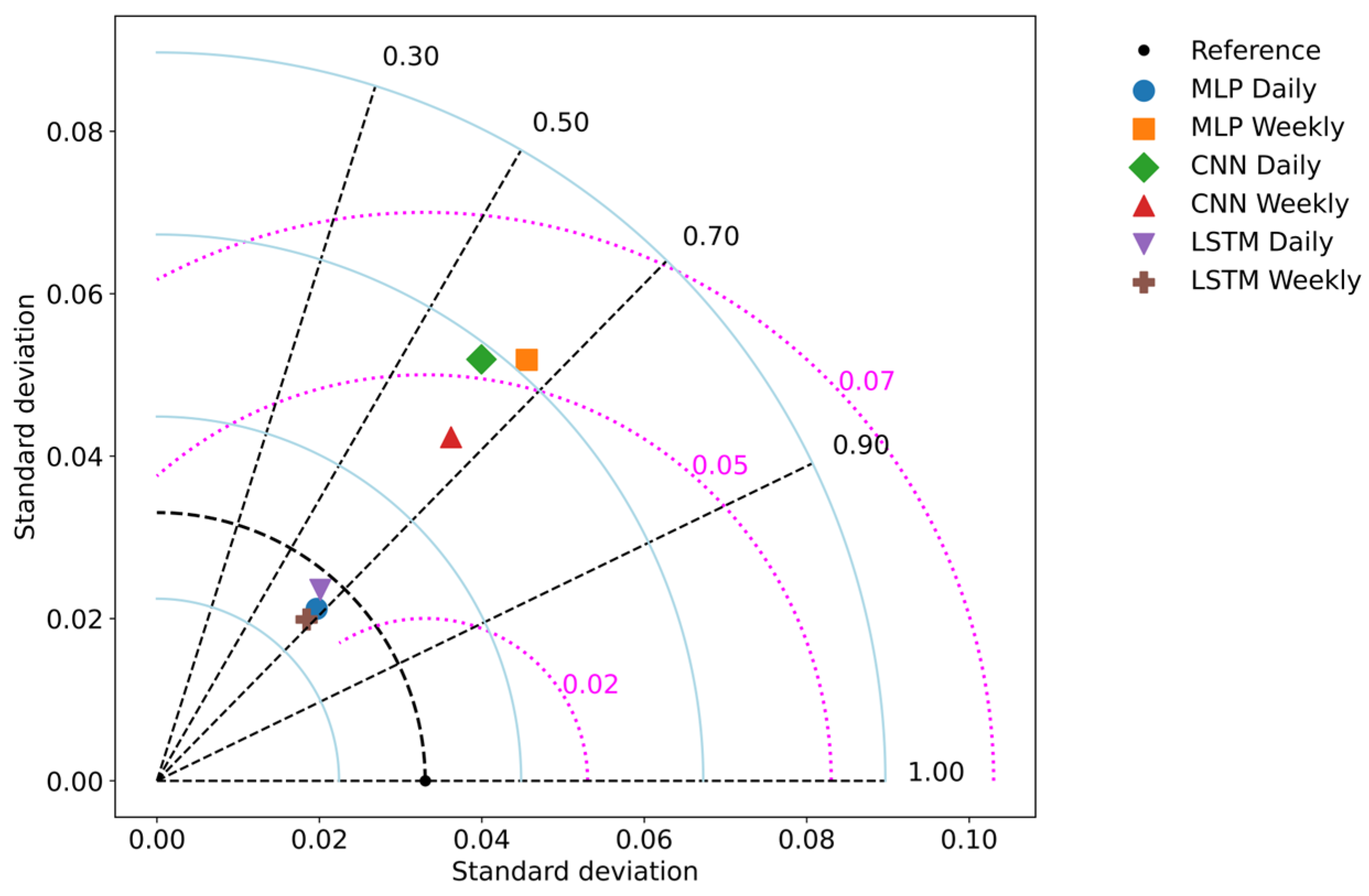
These numerical findings are further illustrated in Figure 22, which provides a Taylor diagram summarizing the performance of MLP, CNN, and LSTM models at daily and weekly time steps (see Table 11 for detailed performance metrics). The black dot and dashed circle indicate the reference standard deviation from observed discharge. Blue arcs represent the standard deviation of model predictions, black dashed rays correspond to correlation coefficients, and magenta dotted arcs denote centered root mean square differences (cRMSD). The diagram is consistent with the numerical results in Table 11: LSTM models (both daily and weekly) are located closest to the reference, demonstrating their ability to reproduce observed variability while maintaining relatively high correlations, thereby offering the best compromise between accuracy and robustness. MLP models show moderate performance, with daily simulations performing better and approaching LSTM performance, while weekly simulations deviate more from the reference. CNN models exhibit the weakest performance overall, particularly at the daily scale, where correlations are markedly lower, although the weekly configuration provides slight improvements in variability representation. Overall, these results emphasize the superiority of recurrent architectures (LSTM) in capturing hydrological dynamics characterized by temporal dependencies and memory effects, whereas feed-forward (MLP) and convolutional (CNN) approaches remain more limited in this regard.
These results align with previous studies highlighting LSTM’s strength in modeling complex temporal dependencies in hydrological systems, especially karst aquifers characterized by significant delayed responses to rainfall [8,24]. Similar trends were reported by [24], who found LSTM networks superior in groundwater level forecasting due to their capability to manage long-term memory effects. Ref. [2] previously demonstrated MLP’s effectiveness for daily scale hydrological predictions, consistent with our findings, while also emphasizing its performance reduction over longer temporal horizons. Conversely, the observed underperformance of CNN in this study contrasts somewhat with findings by [24] who showed moderate CNN efficiency; however, such differences could arise from distinct data characteristics and hydrodynamic complexities of the studied karst systems.

4. Discussion

Our results align with recent literature and offer new insights into the hydrological functioning of semi-arid karst aquifers, particularly their pronounced memory effects and lagged responses. Notably, we observed significant temporal dependencies between climatic variables and the discharge of Jebel Zaghouan, with optimal sequence lengths of 115 to 126 days (approximately four months). Such lags confirm the strong hydrological memory characteristic of semi-arid karst systems, where rainfall infiltrates rapidly through conduits but is released more slowly from the matrix over extended periods [62,63]. Similar memory effects are documented in Mediterranean regions, such as the Fontaine de Vaucluse and Lez springs in southern France [20,64] and Croatian coastal karst springs [22]. Comparable phenomena have also been observed in semi-arid regions like the Zagros Mountains in Iran, where spring discharge lags range from weeks to years, depending on the extent of karstification and aquifer storage capacity [63]. Furthermore, Ref. [65] highlighted multi-scale memory effects in mountainous karst regions, underscoring the necessity of integrating long historical data sequences into predictive models.
Building on these hydrodynamic observations, isotopic and groundwater dating investigations in the Zaghouan karst system in 2021–2022 provided complementary evidence for the coexistence of rapid and delayed flow components [46]. This duality closely reflects the TORCAL model of [61], which characterizes karst systems where temporary storage during recession is followed by gradual release during baseflow, particularly in structurally immature or poorly drained systems. Stable isotope analyses in 2 boreholes (Temple and Ain Ayed 3, 141.5 m and 156 m deep, respectively) of the outflow sampled at weekly step during the rainfall season between September 2021 and April 2022, revealed two different behaviors [53]: a low temporal variability in Temple (Oxygen-18 between −4.96‰ and −5.55‰), indicating a well-mixed system, and in Ain Ayed 3 a larger local temporal variability (δ18O between −5.08‰ and −6.34‰) which could show a direct influence of rainfall at short time step in this borehole (rainfall showing a stronger isotopic variability, and depending on altitude recharge or/and air mass origin). We can hypothesize an efficient blending of the recharge at annual to interannual scales, dampening the isotopic signal. The strong correlation between δ18O and d-excess (R2 = 0.989) in the groundwater suggests a mixing from different karst compartments. While recharge is generally dominant at lower elevations, more depleted isotopic values observed during certain events point to episodic high-altitude contributions. Collectively, these patterns indicate diffuse recharge filtered through structurally complex, weakly connected storage zones, rather than exclusively discrete, event-driven infiltration.
Groundwater dating sampled in September 2022 at 2 sites (EcoMusée and Temple, 256m and 141.5m deep, respectively) reinforces these findings [53]: Tritium concentrations (1.6–1.7 TU) indicated relatively recent recharge (from the last few decades), while radiocarbon data (~63.4% 14C) pointed to much older water (approximately 3000 years BP), evidencing the coexistence of both young and fossil groundwater within a dual-porosity system. The renewal rate inferred from tritium (~1.2–1.3%) and an average residence time of ~80 years further highlighted the slow exchange between mobile and immobile water domains [46].
This hydrodynamic and isotopic framework has direct implications for modeling and prediction using artificial neural networks (ANNs). Given the system’s complex internal storage and memory effects, models capable of representing long-range temporal dependencies are essential. In this context, ANN models implicitly integrate dual recharge regimes and physico-chemical influences on aquifer dynamics, thereby providing a coherent link between short- and long-term memory processes in karst systems. In our modeling experiments, LSTM architectures provided the best overall compromise between short- and long-term forecast reliability [8,59]. For weekly predictions, the LSTM model excelled (KGE’ = 0.64, NSE = 0.50), likely due to its capacity to capture extended temporal dependencies inherent to karst hydrology. This finding aligns with the results of [24] who also found that LSTM models substantially outperformed CNN and MLP architectures in predicting karst spring discharge, especially at weekly to monthly timescales. In contrast, for daily predictions, the MLP performed better (KGE’ = 0.81, NSE = 0.62), consistent with earlier results by [2] who noted high accuracy for short-term forecasts but limitations in capturing longer-term memory effects.
The relatively poor performance of the CNN model in our study—across both temporal scales—contrasts with the moderate results reported in other karst contexts [24,39,59]. This difference can be largely attributed to variations in dataset characteristics and the specific suitability of the models. CNN architectures are primarily designed to extract spatially coherent features and therefore perform better when spatially distributed inputs, such as gridded precipitation or catchment-scale variables, are available [39]. In our case, the dataset was predominantly temporal and lumped, limiting the effectiveness of convolutional filters in capturing relevant patterns. Moreover, the hydrodynamics of the Zaghouan aquifer are dominated by extended temporal dependencies, which are more effectively captured by recurrent architectures such as LSTM [24]. These considerations indicate that CNNs may be most appropriate in hybrid or spatially enriched modeling frameworks, while LSTMs remain preferable for forecasting in strongly memory-driven, semi-arid karst aquifers [59]. Among the three models, MLP and CNN exhibited substantial positive global biases (with a maximum > 55%). This overestimation primarily arises from target-distribution imbalance under low-flow conditions, where rare high-discharge peaks—shaped by prolonged droughts and episodic heavy precipitation—dominate training. When combined with uncertainties in rainfall data, the limited historical discharge records, difficulties in reconstructing temperature and pressure, and structural model limitations, these factors bias the learning process. Under variance-weighted objectives such as NSE, R2, and KGE, errors at moderate to high flows dominate the loss, systematically favoring overestimation at low flows. This is in line with findings by [66], who identified rainfall measurement uncertainty as a major contributor to predictive errors, especially in semi-arid environments with sparse and unevenly distributed data networks. Approaches such as multi-source data integration, bias correction, and advanced gap-filling methods have been shown to enhance model performance under these constraints. For example, Ref. [67] demonstrated that combining gauge, radar, and satellite rainfall data can significantly improve discharge forecasts; in this study, only one rainfall gauge was available. Additionally, recent deep learning-based reconstruction methods, such as EEMD-LSTM, have proved effective in improving historical data recovery and reducing forecast uncertainty [68]. Other strategies can also help mitigate such biases, including stratified sampling or over-sampling of low-flow periods to balance mini-batches, as well as cost-sensitive or quantile-weighted loss functions that assign greater weight to errors under low-flow conditions [69,70].
Overall, ANN-based models generally demonstrated better predictive capability than traditional conceptual models (e.g., KarstMod), especially in data-rich scenarios [39]. Conceptual models offer greater process interpretability and can handle low-flow and recession periods effectively, but often struggle to capture rapid, nonlinear flood events [6]. Indeed, Karstmod reached an NSE of 0.60 over the 1915–1927 period. However, daily discharges were interpolated from infra-weekly data, and evapotranspiration was derived from monthly means distributed uniformly by day. This smoothing procedure limits daily variability, and the model only includes one high peak in the studied period.
The conceptual reservoir model performed slightly lower, with an NSE = 0.54 for the same 1915–1927 period and was subject to the same limitations (interpolated discharge, constant daily ETP, and only one high peak flow event).
Our ANN approach (LSTM) differs in two ways. First, it is trained over a longer period (1915–1944) that includes four distinct high peak events, thus encompassing more hydrological variability. Second, it explicitly integrates daily variability in temperature and pressure, which directly influences evapotranspiration and thus offers a more robust representation of discharge dynamics. The LSTM achieved a KGE′ of 0.62 and an NSE of 0.48 of the same order of magnitude as Karstmod, but with the added benefit of robustness according to KGE′. Since KGE′ is widely recognized as a more balanced diagnostic of hydrological model performance, particularly under variable flow regimes [60], this indicates that the ANN approach provides improved reliability in capturing both low- and high-flow dynamics.
Additionally, ANN models—particularly LSTM—are well suited for representing such rapid and nonlinear events, though they may be less effective during low-flow conditions if such events are underrepresented in the training data [39,59]. Emerging hybrid approaches that combine data-driven and conceptual models have shown promise in bridging these limitations; for example, in the Ljubljanica karst basin, integrating conceptual rainfall-runoff models with machine learning corrections significantly improved flow predictions, particularly during extremes [39]. Furthermore, physics-informed deep learning methods, such as ConvLSTM models that incorporate simulated snow dynamics, further advance predictive accuracy and interpretability by embedding physical processes within ANN architectures [68].
Our findings indicate that the LSTM model offers the most suitable compromise for discharge prediction in karst aquifers, balancing short-term responsiveness and long-term stability. However, the significant biases observed across all ANN models highlight the need for further calibration and the adoption of advanced uncertainty quantification and bias correction methods—such as Monte Carlo dropout or Bayesian approaches—to improve future predictive accuracy [24].
Results show that the karst structure enables temporary water storage in cavities and fissures; however, extraction through boreholes risks prematurely draining these reserves. Intensive pumping accelerates the natural discharge of the system, thereby disrupting the gradual feeding of springs and resurgences. This disruption is even more pronounced in poorly drained systems where limited hydraulic connections slow aquifer replenishment. Under natural conditions, the water stored in the karst aquifer is progressively released, sustaining spring flows during dry periods. Excessive withdrawals reduce this baseflow, increasing the risk of spring desiccation and compromising water availability for both human use and ecosystems.
To ensure sustainable management of the karst system, it is therefore essential to:
  • Limit intensive pumping during low-flow periods by adapting abstraction volumes and establishing seasonal withdrawal quotas with stricter regulation during droughts.
  • Guide withdrawals and predict long-term impacts through regular piezometric monitoring of water levels in wells and spring discharges, together with karst-specific hydrogeological models.
  • Enhance artificial recharge through rainfall infiltration by developing controlled infiltration systems, and by preserving natural recharge to maintain storage.
  • Diversify water supply sources to reduce pressure on the karst aquifer.
This need for sustainable management is further underscored by the fact that the aquifer is currently experiencing a severe hydrological drought [53], impairing its natural functioning and recharge capacity, while ongoing studies aim to assess the potential impacts of climate change on its future dynamics

5. Conclusions

This study highlights the effectiveness of Artificial Neural Networks (ANNs), with a particular focus on the Long Short-Term Memory (LSTM) architecture, in modeling the complex hydrodynamic behavior of the Jebel Zaghouan karst aquifer. Through historical data reconstruction, advanced statistical and probabilistic techniques, we were able to characterize the hydrodynamic functioning of this karstic system. Also, comprehensive comparative analyses of ANN architectures addressed critical challenges in modeling karst aquifers under semi-arid, data-limited conditions.
Results revealed the LSTM model’s superior performance for weekly discharge predictions, successfully capturing the karst system’s characteristic memory effects and delayed hydrological responses. The Multi-Layer Perceptron (MLP) architecture demonstrated robust predictive capability on a daily temporal scale but exhibited significant limitations in forecasting longer-term dynamics. Conversely, the Convolutional Neural Network (CNN) consistently underperformed, underscoring its limited suitability for modeling temporal dependencies inherent in karst hydrology.
Furthermore, integrating isotopic analyses and detailed hydrodynamic evaluations provided crucial insights into the aquifer’s dual recharge mechanisms and internal storage dynamics, strengthening the interpretative capacity of the ANN models. Despite promising outcomes, notable predictive biases were identified, indicating the necessity for enhanced calibration procedures, integrated multi-source data methodologies, and advanced uncertainty quantification approaches in future studies. Additionally, employing alternative data reconstruction techniques, such as hybrid or ensemble methods, could potentially enhance modeling precision and reliability.
Despite its strategic importance as a major groundwater resource in northeastern Tunisia, the hydrodynamic behavior of the Zaghouan karst aquifer remains poorly studied. Its complex recharge mechanisms, significant storage capacity, and sensitivity to climatic variability call for more focused research efforts to support sustainable water management in the region. Indeed, it functions as a temporary storage system, but intensive pumping disrupts its natural discharge, reduces baseflow, and increases the risk of spring desiccation. Sustainable management requires regulated withdrawals, monitoring, artificial recharge, protection of recharge zones, and diversification of water sources to safeguard both water availability and ecosystem health. These findings may also have broader applicability across Mediterranean karst aquifers, where similar hydrological complexities and climatic constraints exist, as demonstrated in studies such as [26,40,44].
In conclusion, this research not only advances methodological approaches essential for sustainable karst water resource management but also underscores the critical importance of historical data preservation. The study provides a scientific basis for informed decision-making and the development of resilient strategies aimed at safeguarding vulnerable groundwater resources amid ongoing climatic variability and anthropogenic pressures.
Future research should also address the interpretability of ANN models, for instance, through explainable Artificial Intelligence approaches such as SHAP, and consider the integration of spatially distributed data within hybrid ANN–conceptual modeling frameworks. Such developments would further improve both the robustness and the transparency of predictions, thereby enhancing their utility for water resource management.

Author Contributions

Conceptualization, E.G.-E., F.S., T.A.O. and J.-D.T.; methodology, E.G.-E. and T.A.O.; software, T.A.O. and E.G.-E.; validation, E.G.-E., F.S. and J.-D.T.; formal analysis, E.G.-E. and T.A.O.; investigation, E.G.-E. and F.S.; resources, E.G.-E., F.S. and J.-D.T.; data curation, E.G.-E. and T.A.O.; writing—original draft, E.G.-E.; writing—review & editing, E.G.-E., T.A.O., F.S., J.-D.T., N.P. and R.B.; visualization, E.G.-E. and T.A.O.; supervision, R.B.; project administration, R.B. and F.S.; funding acquisition, R.B. and F.S. All authors have read and agreed to the published version of the manuscript.

Funding

This research was funded by the General Directorate of Scientific Research in the framework of the PRIMA-KARMA project, grant agreement number 01DH19022A.

Data Availability Statement

The data presented in this study are available on request from the corresponding authors. The data are not publicly available because they are currently used in theses.

Acknowledgments

This Research has been supported by the European Commission through the Partnership for Research and Innovation in the Mediterranean Area (PRIMA) program under Horizon 2020 (KARMA project, grant agreement number 01DH19022A, funded by the General Directorate of Scientific Research for the Tunisian team). We extend our gratitude to the General Directorate of Water Resources (DGRE) for their support, and to the Regional Agricultural Development Commission (CRDA), Zaghouan, for their indispensable facilitation and collaboration. We would like to acknowledge the National Water Exploitation and Distribution Company (SONEDE) for their invaluable support and contributions to this research, particularly the Zaghouan Water Supply Service (SAZ) for their collaboration and assistance in the field, as well as the central laboratory of the Ghdir El Golla water complex for water quality analysis. The authors gratefully acknowledge Lilia Ellouze for her assistance in the colorization of the geological cross-section adapted from [71].

Conflicts of Interest

The authors declare no conflicts of interest. The funders had no role in the design of the study; in the collection, analyses, or interpretation of data; in the writing of the manuscript; or in the decision to publish the results.

Appendix A

Figure A1. Cross-section of Jebel Zaghouan colored and adapted from [71] (Planche IX).
Hydrology 12 00250 g0a1
Figure A2. Title page of the historical meteorological records (1900–1901).
Hydrology 12 00250 g0a2
Figure A3. Example of historical records: monthly rainfall (Bars), hydrograph (line) from 1915 to 1917 at Nymphée Spring.
Hydrology 12 00250 g0a3
Figure A4. Data splitting strategy.
Hydrology 12 00250 g0a4
Table A1. Rainfall characteristics.
Rainfall (mm/year)Zaghouan ContrôleZaghouan SM
Minimum252230
Maximum994927
Average520503
Median507506
Standard deviation170168
Table A2. Interpretation of slope breaks in the ranked flow curves according [61].
ClassificationSlope of the LinesPosition of the BreakInterpretation
Aα2 > α1High percentagesOperation of overflow
Leaks to another system
Temporary storage
Leaks or overflow of the gauging station during high water
Bα2 < α1High percentagesInflows from another system
The gauging station accounts during floods for flows not belonging to the system
Cα2 > α1Low percentagesFormation of a reserve
Dα2 < α1Low percentagesContribution of a reserve from a previous cycle
Eα2 > α3
and
α1 < α2
Double breakTrapping of a reserve during recession and restitution during the drying up

Appendix B

Appendix B.1. Multi-Layer Perceptron (MLP) Model

A Multilayer Perceptron (MLP) is a nonlinear statistical learning architecture composed of interconnected layers of neurons, typically structured as an input layer, one or several hidden layers, and an output layer [72]. Each neuron within a given layer is fully connected to every neuron in the subsequent layer, forming a dense network of computational nodes. Hidden layer neurons apply nonlinear activation functions, such as sigmoid, hyperbolic tangent, or rectified linear unit (ReLU), enabling the network to model complex and nonlinear relationships between input variables and outputs [73].
MLPs are widely employed due to their capability of universal function approximation, meaning they can approximate almost any continuous function, providing enough neurons and layers [74]. In hydrological modeling, especially in karst hydrodynamics, this flexibility allows the MLP to capture intricate interactions between hydrological inputs (e.g., rainfall, infiltration rates) and outputs (e.g., spring discharge) [2].
Specifically, MLPs have been successfully applied in karst modeling to predict spring discharge, water level fluctuations, and contaminant transport by integrating various hydrological inputs and meteorological variables [34,75,76]. Their strength lies in handling noisy, incomplete data often encountered in karst systems due to their heterogeneous and anisotropic characteristics. Furthermore, MLP models have demonstrated potential in real-time forecasting and management of water resources in karst regions [77].
Despite their versatility, MLP models require careful consideration regarding their architecture, training methods, and regularization techniques to avoid issues such as overfitting and to ensure robust generalization performance [78].

Appendix B.2. CNN Model

CNN models introduced by [79] are widely recognized for their efficacy in image recognition and classification tasks. However, they have also demonstrated strong performance in signal processing applications and natural language processing tasks. CNN models are typically composed of three main types of layers: convolutional, pooling, and fully connected dense layers.
The convolutional layers, the foundational components of CNNs, utilize filters to process input data. Each filter operates over a specific region of the input, known as the receptive field, and is systematically applied across the entire input to produce an output feature map. The pooling layers, often placed after convolutional layers, downsample the feature maps by summarizing information within receptive fields using operations such as averaging or selecting maximum values. This process consolidates information and reduces the dimensionality of the feature maps.
Similarly to LSTM networks, CNN architectures can involve stacking multiple convolutional and pooling layers in various configurations to create deeper models. The final layer is typically a fully connected dense layer, which outputs predictions. For sequence forecasting tasks, the dense layer contains as many output neurons as the number of time steps in the target sequence.

Appendix B.3. LSTM Models

LSTM models are part of recurrent neural networks (RNNs) and are applied to sequential time series data [80]. LSTMs are designed to overcome the limitation of vanishing gradient problems during backpropagation through memory limitation to approximately 10 time steps [80].
In their architecture, LSTM models integrate a cell memory or cell state in addition to the hidden state. These are combined with specialized gates: forget gate, input gate, and output gate to regulate information flow [80].
The forget gate keeps essential information from cell memory, which means it discards some information from cell memory [81]. The input gate governs the incorporation of new inputs into the cell memory, and the output gate controls the contribution of cell memory elements to the LSTM cell’s hidden state. These mechanisms enable LSTM models to effectively capture long-term dependencies, as information can persist in the memory across multiple time steps.
In practice, multiple LSTM layers can be stacked within a model to enhance representational capacity. The final LSTM layer typically connects to a fully connected dense layer. For sequence forecasting tasks, the dense layer includes as many output neurons as the desired sequence length. In the context of this study, the dense layer contains a single output neuron to predict groundwater levels.

Appendix B.4. Hyperparameter Tuning Procedure

Hyperparameter tuning is crucial in optimizing the performance of machine learning models. One of the methods used for hyperparameter tuning is Bayesian optimization, which is a powerful and efficient strategy frequently used for hyperparameter tuning. It employs probabilistic models (e.g., Gaussian processes) to systematically explore the hyperparameter space, balancing exploration and exploitation to identify optimal hyperparameter configurations quickly [82].
In the context of neural networks, critical hyperparameters such as batch size, dropout rate, and learning rate have been widely investigated in the literature. Batch size influences the stability and convergence speed of training; smaller batches typically enhance generalization but at the cost of computational efficiency [83]. Dropout rate serves as a regularization technique, preventing overfitting by randomly disabling neurons during training, thus forcing the network to develop redundant representations [84]. Learning rate significantly impacts convergence and final accuracy, requiring careful tuning to ensure efficient and stable learning [73].
Bayesian optimization is a powerful and efficient strategy frequently used for hyperparameter tuning. It employs probabilistic models, typically Gaussian processes, to systematically explore the hyperparameter space, balancing exploration (evaluating new points in parameter space) and exploitation (focusing on known promising areas). Bayesian optimization iteratively updates the posterior distribution of the performance metric to guide subsequent hyperparameter choices effectively [82].
The Bayesian optimization process involves:
  • Defining an objective function representing the model’s performance.
  • Constructing a probabilistic surrogate model, typically a Gaussian Process (GP), that approximates.
  • Selecting the next hyperparameter configuration x to evaluate by optimizing an acquisition function, such as Expected Improvement (EI, Equation (A1)), given by:
EI x = E max 0 , f x f x
where x∗ represents the best configuration found so far. Additionally, sequence length, another crucial hyperparameter in our hydrodynamic modeling, was fine-tuned based on our statistical analysis of the input data to ensure the model captures essential temporal dynamics specific to karst hydrological processes according to the dependence between climatic data and discharge.

Appendix B.5. Bayesian Optimization Convergence Plots
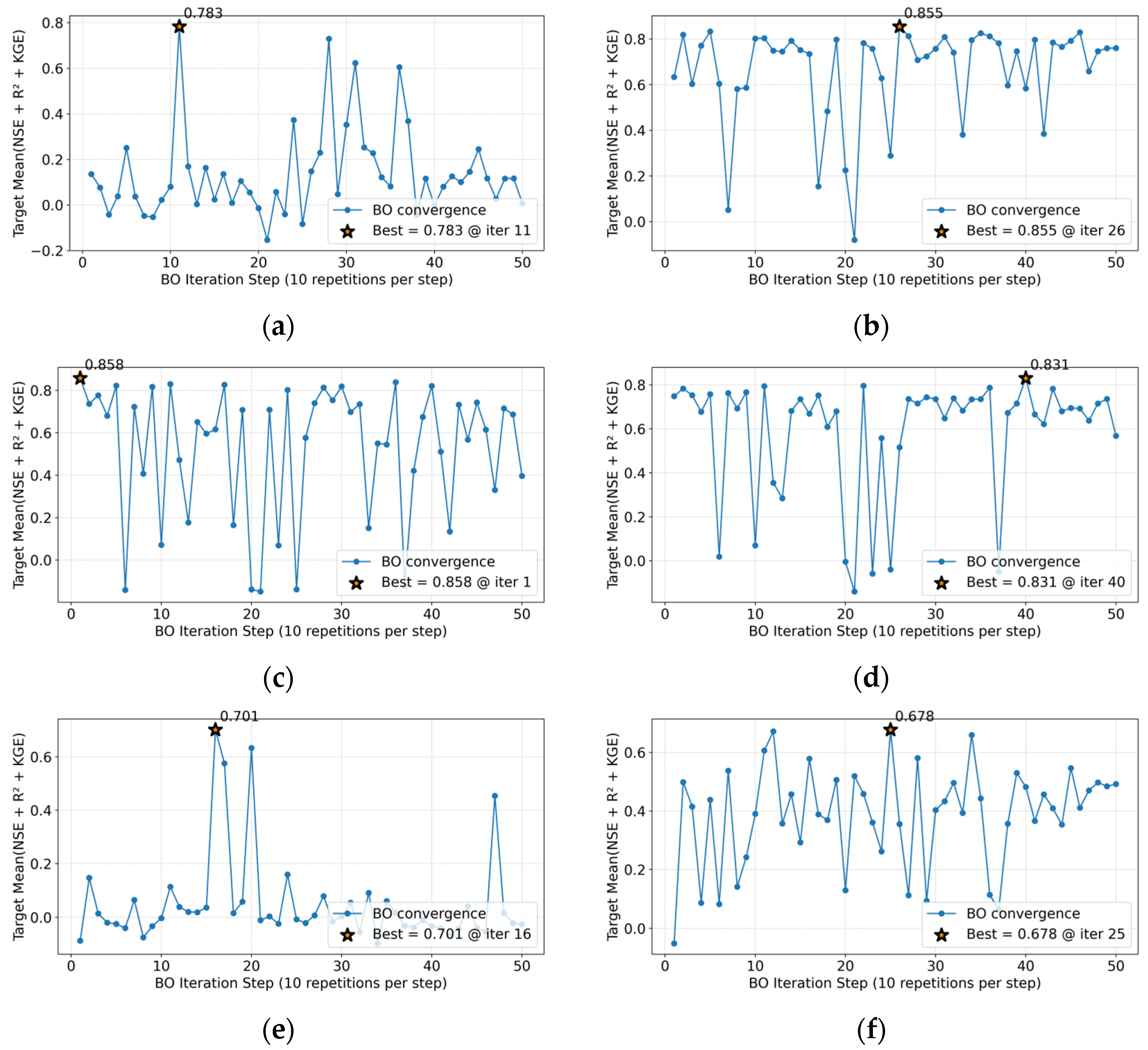
Figure A5. Bayesian optimization convergence plot 50 iterations (a) MLP Daily; (b) MLP Weekly; (c) CNN Daily; (d) CNN Weekly; (e) LSTM Daily; (f) LSTM Weekly.
Hydrology 12 00250 g0a5

References

  1. Ford, D.; Williams, P.W. Karst Hydrogeology and Geomorphology; John Wiley & Sons: Chichester, UK; Hoboken, NJ, USA, 2007; ISBN 978-0-470-84996-5. [Google Scholar]
  2. Kurtulus, B.; Razack, M. Modeling Daily Discharge Responses of a Large Karstic Aquifer Using Soft Computing Methods: Artificial Neural Network and Neuro-Fuzzy. J. Hydrol. 2010, 381, 101–111. [Google Scholar] [CrossRef]
  3. Bakalowicz, M. Karst and Karst Groundwater Resources in the Mediterranean. Environ. Earth Sci. 2015, 74, 5–14. [Google Scholar] [CrossRef]
  4. Jourde, H.; Wang, X. Advances, Challenges and Perspective in Modelling the Functioning of Karst Systems: A Review. Environ. Earth Sci. 2023, 82, 396. [Google Scholar] [CrossRef]
  5. Ghasemizadeh, R.; Hellweger, F.; Butscher, C.; Padilla, I.; Vesper, D.; Field, M.; Alshawabkeh, A. Review: Groundwater Flow and Transport Modeling of Karst Aquifers, with Particular Reference to the North Coast Limestone Aquifer System of Puerto Rico. Hydrogeol. J. 2012, 20, 1441–1461. [Google Scholar] [CrossRef] [PubMed]
  6. Rehrl Christoph; Birk Steffen Hydrogeological Characterisation and Modelling of Spring Catchments in a Changing Environment. Austrian J. Earth Sci. 2010, 103, 106–117.
  7. Bakalowicz, M. Karst Groundwater: A Challenge for New Resources. Hydrogeol. J. 2005, 13, 148–160. [Google Scholar] [CrossRef]
  8. Zhou, R.; Zhang, Y. Linear and Nonlinear Ensemble Deep Learning Models for Karst Spring Discharge Forecasting. J. Hydrol. 2023, 627, 130394. [Google Scholar] [CrossRef]
  9. Jeannin, P.-Y.; Artigue, G.; Butscher, C.; Chang, Y.; Charlier, J.-B.; Duran, L.; Gill, L.; Hartmann, A.; Johannet, A.; Jourde, H.; et al. Karst Modelling Challenge 1: Results of Hydrological Modelling. J. Hydrol. 2021, 600, 126508. [Google Scholar] [CrossRef]
  10. Johannet, A.; Taver, V.; Kong-A-Siou, L.; Borrell, V.; Pistre, S.; Mangin, A.; Vayssade, B.; Vinches, M.; Bertin, D. Les réseaux de neurones artificiels pour la modélisation hydrodynamique des aquifères karstiques: Présentation générale et illustrations. Karstologia 2012, 60, 45–59. [Google Scholar] [CrossRef]
  11. Kovács, A. Geometry and Hydraulic Parameters of Karst Aquifers: A Hydrodynamic Modeling Approach. Ph.D. Thesis, Université de Neuchâtel, Neuchâtel, Switzerland, 2003. [Google Scholar]
  12. Sezen, C.; Bezak, N.; Bai, Y.; Šraj, M. Hydrological Modelling of Karst Catchment Using Lumped Conceptual and Data Mining Models. J. Hydrol. 2019, 576, 98–110. [Google Scholar] [CrossRef]
  13. Methods in Karst Hydrogeology; Goldscheider, N., Drew, D., Eds.; CRC Press: Boca Raton, FL, USA, 2014; ISBN 978-0-429-15341-9. [Google Scholar] [CrossRef]
  14. Mazzilli, N.; Guinot, V.; Jourde, H.; Lecoq, N.; Labat, D.; Arfib, B.; Baudement, C.; Danquigny, C.; Dal Soglio, L.; Bertin, D. KarstMod: A Modelling Platform for Rainfall—Discharge Analysis and Modelling Dedicated to Karst Systems. Environ. Model. Softw. 2019, 122, 103927. [Google Scholar] [CrossRef]
  15. Kovács, A.; Sauter, M. Modelling Karst Hydrodynamics. In Methods in Krast Hydrogeology; CRC Press: Boca Raton, FL, USA, 2007; Chapter 10; pp. 201–222. [Google Scholar]
  16. Lee, E.S.; Krothe, N.C. A Four-Component Mixing Model for Water in a Karst Terrain in South-Central Indiana, USA. Using Solute Concentration and Stable Isotopes as Tracers. Chem. Geol. 2001, 179, 129–143. [Google Scholar] [CrossRef]
  17. Döerfliger, N.; Jeannin, P.-Y.; Zwahlen, F. Water Vulnerability Assessment in Karst Environments: A New Method of Defining Protection Areas Using a Multi-Attribute Approach and GIS Tools (EPIK Method). Environ. Geol. 1999, 39, 165–176. [Google Scholar] [CrossRef]
  18. Jeannin, P.-Y.; Sauter, M. Analysis of Karst Hydrodynamic Behavior Using Global Approaches: A Review. Bull. Hydrogéol. 1998, 16, 31–48. [Google Scholar]
  19. Salerno, F.; Tartari, G. A Coupled Approach of Surface Hydrological Modelling and Wavelet Analysis for Understanding the Baseflow Components of River Discharge in Karst Environments. J. Hydrol. 2009, 376, 295–306. [Google Scholar] [CrossRef]
  20. Fleury, P.; Ladouche, B.; Conroux, Y.; Jourde, H.; Dörfliger, N. Modelling the Hydrologic Functions of a Karst Aquifer under Active Water Management—The Lez Spring. J. Hydrol. 2009, 365, 235–243. [Google Scholar] [CrossRef]
  21. De Vos, N.J.; Rientjes, T.H.M. Multi-Objective Performance Comparison of an Artificial Neural Network and a Conceptual Rainfall—Runoff Model. Hydrol. Sci. J. 2007, 52, 397–413. [Google Scholar] [CrossRef]
  22. Denić-Jukić, V.; Jukić, D. Composite Transfer Functions for Karst Aquifers. J. Hydrol. 2003, 274, 80–94. [Google Scholar] [CrossRef]
  23. Hartmann, A.; Gleeson, T.; Rosolem, R.; Pianosi, F.; Wada, Y.; Wagener, T. A Simulation Model to Assess Groundwater Recharge over Europe’s Karst Regions. Geosci. Model Dev. Discuss. 2014, 7, 7887–7935. [Google Scholar] [CrossRef]
  24. Wunsch, A.; Liesch, T.; Cinkus, G.; Ravbar, N.; Chen, Z.; Mazzilli, N.; Jourde, H.; Goldscheider, N. Karst Spring Discharge Modeling Based on Deep Learning Using Spatially Distributed Input Data. Hydrol. Earth Syst. Sci. 2022, 26, 2405–2430. [Google Scholar] [CrossRef]
  25. Hartmann, A.; Gleeson, T.; Rosolem, R.; Pianosi, F.; Wada, Y.; Wagener, T. A Large-Scale Simulation Model to Assess Karstic Groundwater Recharge over Europe and the Mediterranean. Geosci. Model Dev. 2015, 8, 1729–1746. [Google Scholar] [CrossRef]
  26. Bertola, M.; Mazzoglio, P.; HELPING REHYDRATE working group. REHYDRATE—An International HELPING Working Group to REtrieve Historical HYDRologic dATa and Estimates. Available online: https://www.researchgate.net/publication/379980552_REHYDRATE_-_an_international_HELPING_working_group_to_REtrieve_historical_HYDRologic_dATa_and_Estimates (accessed on 22 September 2025). [CrossRef]
  27. Cinkus, G.; Mazzilli, N.; Jourde, H. Identification of Relevant Indicators for the Assessment of Karst Systems Hydrological Functioning: Proposal of a New Classification. J. Hydrol. 2021, 603, 127006. [Google Scholar] [CrossRef]
  28. Chen, X.; Zhang, Z.; Soulsby, C.; Cheng, Q.; Binley, A.; Jiang, R.; Tao, M. Characterizing the Heterogeneity of Karst Critical Zone and Its Hydrological Function: An Integrated Approach. Hydrol. Process. 2018, 32, 2932–2946. [Google Scholar] [CrossRef]
  29. An, L.; Hao, Y.; Yeh, T.-C.J.; Liu, Y.; Liu, W.; Zhang, B. Simulation of Karst Spring Discharge Using a Combination of Time–Frequency Analysis Methods and Long Short-Term Memory Neural Networks. J. Hydrol. 2020, 589, 125320. [Google Scholar] [CrossRef]
  30. Bergen, K.J.; Johnson, P.A.; De Hoop, M.V.; Beroza, G.C. Machine Learning for Data-Driven Discovery in Solid Earth Geoscience. Science 2019, 363, eaau0323. [Google Scholar] [CrossRef] [PubMed]
  31. Gholami, V.; Khaleghi, M.R. A Comparative Study of the Performance of Artificial Neural Network and Multivariate Regression in Simulating Springs Discharge in the Caspian Southern Watersheds, Iran. Appl. Water Sci. 2019, 9, 9. [Google Scholar] [CrossRef]
  32. Trichakis, I.C.; Nikolos, I.K.; Karatzas, G.P. Artificial Neural Network (ANN) Based Modeling for Karstic Groundwater Level Simulation. Water Resour. Manag. 2011, 25, 1143–1152. [Google Scholar] [CrossRef]
  33. Paleologos, E.K.; Skitzi, I.; Katsifarakis, K.; Darivianakis, N. Neural Network Simulation of Spring Flow in Karst Environments. Stoch. Environ. Res. Risk Assess. 2013, 27, 1829–1837. [Google Scholar] [CrossRef]
  34. Kong-A-Siou, L.; Johannet, A.; Borrell Estupina, V.; Pistre, S. Neural Networks for Karst Groundwater Management: Case of the Lez Spring (Southern France). Environ. Earth Sci 2015, 74, 7617–7632. [Google Scholar] [CrossRef]
  35. Opoku, P.A.; Shu, L.; Ansah-Narh, T.; Banahene, P.; Yao, K.B.M.O.; Kwaw, A.K.; Niu, S. Prediction of Karst Spring Discharge Using LSTM with Bayesian Optimisation Hyperparameter Tuning: A Laboratory Physical Model Approach. Model. Earth Syst. Environ. 2024, 10, 1457–1482. [Google Scholar] [CrossRef]
  36. Kharroubi, O.; Achour, R.; Ammami, M.-T.; Benamar, A. Hourly Flow Forecasting in a Karst Watershed: The Iton River (France). Water 2025, 17, 977. [Google Scholar] [CrossRef]
  37. De Filippi, F.M.; Ginesi, M.; Sappa, G. A Fully Connected Neural Network (FCNN) Model to Simulate Karst Spring Flowrates in the Umbria Region (Central Italy). Water 2024, 16, 2580. [Google Scholar] [CrossRef]
  38. Fasihi, R.; Taheri Tizro, A.; Marofi, S. Simulating the Discharge of Nahavand Karstic Springs Based on Neural Intelligent Models. J. Hydroinform. 2025, 27, 442–455. [Google Scholar] [CrossRef]
  39. Cinkus, G.; Wunsch, A.; Mazzilli, N.; Liesch, T.; Chen, Z.; Ravbar, N.; Doummar, J.; Fernández-Ortega, J.; Barberá, J.A.; Andreo, B.; et al. Comparison of Artificial Neural Networks and Reservoir Models for Simulating Karst Spring Discharge on Five Test Sites in the Alpine and Mediterranean Regions. Hydrol. Earth Syst. Sci. 2023, 27, 1961–1985. [Google Scholar] [CrossRef]
  40. Mo, C.; Jiang, C.; Lei, X.; Lai, S.; Deng, Y.; Cen, W.; Sun, G.; Xing, Z. Combining Standard Artificial Intelligence Models, Pre-Processing Techniques, and Post-Processing Methods to Improve the Accuracy of Monthly Runoff Predictions in Karst-Area Watersheds. Appl. Sci. 2022, 13, 88. [Google Scholar] [CrossRef]
  41. Djebbi, M.; Besbes, M.; Sagna, J.; Rekaya, M. The Karstic Springs from Zaghouan. Looking for a Rainfall-Discharge Operator; Univ. Franche-Comté: Besançon, France, 2001; pp. 125–128. [Google Scholar]
  42. Nazoumou, Y. Study of the Deep Aquifers of the South-Eastern Governorate of Zaghouan (Tunisia); Water Resources Directorate/SCET: Tunis, Tunisia, 2002; p. 100. [Google Scholar]
  43. Zhou, G.; Yan, H.; Chen, K.; Zhang, R. Spatial Analysis for Susceptibility of Second-Time Karst Sinkholes: A Case Study of Jili Village in Guangxi, China. Comput. Geosci. 2016, 89, 144–160. [Google Scholar] [CrossRef]
  44. Fadhillah, M.F.; Lee, S.; Lee, C.-W.; Park, Y.-C. Application of Support Vector Regression and Metaheuristic Optimization Algorithms for Groundwater Potential Mapping in Gangneung-Si, South Korea. Remote Sens. 2021, 13, 1196. [Google Scholar] [CrossRef]
  45. Reimann, T.; Hill, M.E. MODFLOW-CFP: A New Conduit Flow Process for MODFLOW–2005. Groundwater 2009, 47, 321–325. [Google Scholar] [CrossRef]
  46. Birk, S.; Liedl, R.; Sauter, M. Karst Spring Responses Examined by Process-Based Modeling. Groundwater 2006, 44, 832–836. [Google Scholar] [CrossRef] [PubMed]
  47. Instituto Geológico y Minero de España (IGME); Pardo-Igúzquiza, E.; Dowd, P.; The University of Adelaide; Durán, J.; Robledo-Ardila, P.; Unidad del IGME en las Islas Baleares. A Review of Fractals in Karst. IJS 2019, 48, 11–20. [Google Scholar] [CrossRef]
  48. Mangin, A. Contribution à L’étude Hydrodynamique des Aquifères Karstiques. Ph.D. Thesis, Sciences de la Terre, Université de Dijon, Dijon, France, 1975. [Google Scholar]
  49. Fandel, C.; Ferré, T.; Miville, F.; Renard, P.; Goldscheider, N. Improving Understanding of Groundwater Flow in an Alpine Karst System by Reconstructing Its Geologic History Using Conduit Network Model Ensembles. Hydrol. Earth Syst. Sci. 2023, 27, 4205–4215. [Google Scholar] [CrossRef]
  50. PRIMA-KARMA Project. The KARMA Project. Retrieved from Karst Aquifer Resources Availability and Quality in the Mediterranean Area. 2023. Available online: http://karma-project.org/ (accessed on 1 January 2019).
  51. Faydi, T. La Modélisation Hydrodynamique des Aquifères Karstiques de Djebel Zaghouan par KarstMod. Master’s Thesis, University Tunis El Manar, National Engineering School of Tunis, Tunis, Tunisia, 2021. Available online: https://www.biruni.tn/catalogue-local.php?ei=29 (accessed on 22 September 2025).
  52. Clamagirand, E.; Rais, S.; Chahed, J.; Guefrej, R.; Smaoui, L. L’aqueduc de Carthage. La Houille Blanche 1990, 76, 423–432. [Google Scholar] [CrossRef]
  53. Gargouri-Ellouze, E.; Slama, F.; Kriaa, S.; Benhmid, A.; Taupin, J.-D.; Bouhlila, R. Comprehensive Assessment of the Jebel Zaghouan Karst Aquifer (Northeastern Tunisia): Availability, Quality, and Vulnerability, in the Context of Overexploitation and Global Change. Water 2025, 17, 407. [Google Scholar] [CrossRef]
  54. Franzke, C.L.E.; Barbosa, S.; Blender, R.; Fredriksen, H.; Laepple, T.; Lambert, F.; Nilsen, T.; Rypdal, K.; Rypdal, M.; Scotto, M.G.; et al. The Structure of Climate Variability Across Scales. Rev. Geophys. 2020, 58, e2019RG000657. [Google Scholar] [CrossRef]
  55. North, G.R.; Wang, J.; Genton, M.G. Correlation Models for Temperature Fields. J. Clim. 2011, 24, 5850–5862. [Google Scholar] [CrossRef]
  56. Niako, N.; Melgarejo, J.D.; Maestre, G.E.; Vatcheva, K.P. Effects of Missing Data Imputation Methods on Univariate Blood Pressure Time Series Data Analysis and Forecasting with ARIMA and LSTM. BMC Med. Res. Methodol. 2024, 24, 320. [Google Scholar] [CrossRef]
  57. Mangin, A. Pour une meilleure connaissance des systèmes hydrologiques à partir des analyses corrélatoire et spectrale. J. Hydrol. 1984, 67, 25–43. [Google Scholar] [CrossRef]
  58. Siou, L.K.a. Modélisation des Crues de Bassins Karstiques par Réseaux de Neurones. Cas du Bassin du Lez (France). Ph.D. Thesis, Université Montpellier II—Sciences et Techniques du Languedoc, Montpellier, France, 2011. Available online: https://theses.hal.science/tel-00649103v1 (accessed on 22 September 2025).
  59. Wunsch, A.; Liesch, T.; Broda, S. Groundwater Level Forecasting with Artificial Neural Networks: A Comparison of Long Short-Term Memory (LSTM), Convolutional Neural Networks (CNNs), and Non-Linear Autoregressive Networks with Exogenous Input (NARX). Hydrol. Earth Syst. Sci. 2021, 25, 1671–1687. [Google Scholar] [CrossRef]
  60. Gupta, H.V.; Kling, H.; Yilmaz, K.K.; Martinez, G.F. Decomposition of the Mean Squared Error and NSE Performance Criteria: Implications for Improving Hydrological Modelling. J. Hydrol. 2009, 377, 80–91. [Google Scholar] [CrossRef]
  61. Marsaud, B. Structure et Fonctionnement de la Zone Noyée des Karsts à Partir des Résultats Expérimentaux. Ph.D. Thesis, Université Paris IX, Orsay, France, 1997. [Google Scholar]
  62. Hartmann, A.; Liu, Y.; Olarinoye, T.; Berthelin, R.; Marx, V. Integrating Field Work and Large-Scale Modeling to Improve Assessment of Karst Water Resources. Hydrogeol. J. 2021, 29, 315–329. [Google Scholar] [CrossRef]
  63. Sivelle, V.; Cinkus, G.; Mazzilli, N.; Labat, D.; Arfib, B.; Massei, N.; Cousquer, Y.; Bertin, D.; Jourde, H. Improvement of the KarstMod Modelling Platform for a Better Assessment of Karst Groundwater Resources. Hydrol. Earth Syst. Sci. 2025, 29, 1259–1276. [Google Scholar] [CrossRef]
  64. Fleury, P.; Plagnes, V.; Bakalowicz, M. Modelling of the Functioning of Karst Aquifers with a Reservoir Model: Application to Fontaine de Vaucluse (South of France). J. Hydrol. 2007, 345, 38–49. [Google Scholar] [CrossRef]
  65. Tennant, H.; Neilson, B.T.; Hill, D.; Newell, D.L.; Evans, J.P.; Choi, S.; McNamara, J.P.; Ashmead, N.; Xu, T. Karst Hydrologic Memory Supplements Streamflow During Dry Periods in Snow-Dominated, Mountainous Watersheds. Hydrol. Process. 2024, 38, e70019. [Google Scholar] [CrossRef]
  66. Baig, F.; Sherif, M.; Faiz, M.A. Quantification of Precipitation and Evapotranspiration Uncertainty in Rainfall-Runoff Modeling. Hydrology 2022, 9, 51. [Google Scholar] [CrossRef]
  67. Min, X.; Yang, C.; Dong, N. Merging Satellite and Gauge Rainfalls for Flood Forecasting of Two Catchments Under Different Climate Conditions. Water 2020, 12, 802. [Google Scholar] [CrossRef]
  68. Xu, G.; Fan, H.; Oliver, D.M.; Dai, Y.; Li, H.; Shi, Y.; Long, H.; Xiong, K.; Zhao, Z. Decoding River Pollution Trends and Their Landscape Determinants in an Ecologically Fragile Karst Basin Using a Machine Learning Model. Environ. Res. 2022, 214, 113843. [Google Scholar] [CrossRef]
  69. Feng, D.; Fang, K.; Shen, C. Enhancing Streamflow Forecast and Extracting Insights Using Long-Short Term Memory Networks With Data Integration at Continental Scales. Water Resour. Res. 2020, 56, e2019WR026793. [Google Scholar] [CrossRef]
  70. Kratzert, F.; Klotz, D.; Herrnegger, M.; Sampson, A.K.; Hochreiter, S.; Nearing, G.S. Toward Improved Predictions in Ungauged Basins: Exploiting the Power of Machine Learning. Water Resour. Res. 2019, 55, 11344–11354. [Google Scholar] [CrossRef]
  71. Castany, G. Etude Géologique de l’Atlas Tunisien Oriental; Annales des mines et de la géologie. Régence de Tunis Protectorat français Direction des travaux publics; Imprimerie de l’Est: Besançon, France, 1951; Available online: https://www.onm.nat.tn/fr/index.php?p=notices&findtype=details&id=9849 (accessed on 22 September 2025).
  72. Bishop, C.M. Pattern Recognition and Machine Learning; Information science and statistics; Springer: New York, NY, USA, 2006; ISBN 978-0-387-31073-2. [Google Scholar]
  73. Goodfellow, I.; Bengio, Y.; Courville, A. Deep Learning; Adaptive Computation and Machine Learning; The MIT Press: Cambridge, MA, USA, 2016; ISBN 978-0-262-03561-3. [Google Scholar]
  74. Hornik, K.; Stinchcombe, M.; White, H. Multilayer Feedforward Networks Are Universal Approximators. Neural Netw. 1989, 2, 359–366. [Google Scholar] [CrossRef]
  75. Kisi, O.; Shiri, J.; Tombul, M. Modeling Rainfall-Runoff Process Using Soft Computing Techniques. Comput. Geosci. 2013, 51, 108–117. [Google Scholar] [CrossRef]
  76. Tzoraki, O.; Nikolaidis, N.P. A Generalized Framework for Modeling the Hydrologic and Biogeochemical Response of a Mediterranean Temporary River Basin. J. Hydrol. 2007, 346, 112–121. [Google Scholar] [CrossRef]
  77. Cheng, S.; Qiao, X.; Shi, Y.; Wang, D. Machine Learning for Predicting Discharge Fluctuation of a Karst Spring in North China. Acta Geophys. 2021, 69, 257–270. [Google Scholar] [CrossRef]
  78. Piotrowski, A.P.; Napiorkowski, J.J. A Comparison of Methods to Avoid Overfitting in Neural Networks Training in the Case of Catchment Runoff Modelling. J. Hydrol. 2013, 476, 97–111. [Google Scholar] [CrossRef]
  79. LeCun, Y.; Bengio, Y.; Hinton, G. Deep Learning. Nature 2015, 521, 436–444. [Google Scholar] [CrossRef]
  80. Hochreiter, S.; Schmidhuber, J. Long Short-Term Memory. Neural Comput. 1997, 9, 1735–1780. [Google Scholar] [CrossRef]
  81. Gers, F.A.; Schmidhuber, J.; Cummins, F. Learning to Forget: Continual Prediction with LSTM. Neural Comput. 2000, 12, 2451–2471. [Google Scholar] [CrossRef]
  82. Snoek, J.; Larochelle, H.; Adams, R.P. Practical Bayesian Optimization of Machine Learning Algorithms. Adv. Neural Inf. Process. Syst. 2012, 25. [Google Scholar] [CrossRef]
  83. Keskar, N.S.; Mudigere, D.; Nocedal, J.; Smelyanskiy, M.; Tang, P.T.P. On Large-Batch Training for Deep Learning: Generalization Gap and Sharp Minima. arXiv 2016. [Google Scholar] [CrossRef]
  84. Srivastava, N.; Hinton, G.; Krizhevsky, A.; Sutskever, I.; Salakhutdinov, R. Dropout: A Simple Way to Prevent Neural Networks from Overfitting. J. Mach. Learn. Res. 2014, 15, 1929–1958. [Google Scholar]
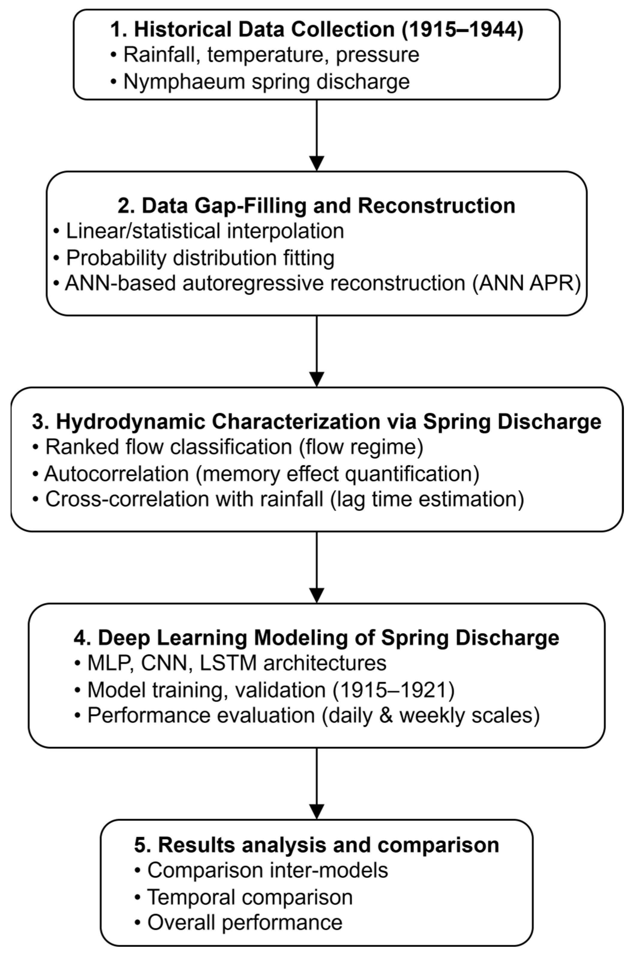
Figure 1. Study workflow.
Hydrology 12 00250 g001
Figure 2. Location of study area (Tunisia in green; Zaghouan Governorate in orange; Right: Zahgouan Karst topographic map).
Hydrology 12 00250 g002
Figure 3. Geological context of Jebel Zaghouan (Cross-section Figure A1, in the Appendix A).
Hydrology 12 00250 g003
Figure 4. Integrated hydrological map: hydrological network, wells, springs, rainfall stations, and spatial distribution of precipitation.
Hydrology 12 00250 g004
Figure 5. Precipitation and spring discharges of Nymphée spring for the period 1915–1943.
Hydrology 12 00250 g005
Figure 6. (a) Correlation of mean daily temperature between Tunis and Zaghouan stations from 2000 to 2005; (b) Correlation of mean daily atmospheric pressure between Tunis and Zaghouan stations from 2000 to 2005.
Hydrology 12 00250 g006
Figure 7. Historical data: (a) daily mean temperature; (b) daily mean pressure.
Hydrology 12 00250 g007
Figure 8. Digitized discharges (after processing).
Hydrology 12 00250 g008
Figure 9. Autocorrelation of discharge at different temporal scales: (a) daily; (b) weekly; (c) monthly.
Hydrology 12 00250 g009
Figure 10. Lag time using cross correlation between rainfall and discharge at different temporal scales (a) daily; (b) weekly; (c) monthly.
Hydrology 12 00250 g010
Figure 11. MLP model (a) daily; (b) weekly.
Hydrology 12 00250 g011
Figure 12. CNN model (a) daily; (b) weekly.
Hydrology 12 00250 g012
Figure 13. LSTM model (a) daily; (b) weekly.
Hydrology 12 00250 g013
Figure 14. Annual rainfall correlation between Zaghouan Contrôle and Zaghouan SM.
Hydrology 12 00250 g014
Figure 15. Quarterly correlation between Zaghouan Contrôle and Zaghouan SM (a) First trimester; (b) Second trimester; (c) Third trimester; (d) Fourth trimester.
Hydrology 12 00250 g015
Figure 16. (a) daily rainfall with gaps; (b) without gaps from 1915 to 1944 at Zaghouan Contrôle Station.
Hydrology 12 00250 g016
Figure 17. Reconstitution with PDR (a) daily mean temperature at Tunis station; (b) daily mean temperature at Zaghouan station; (c) daily mean pressure at Tunis station; (d) daily mean pressure at Zaghouan station.
Hydrology 12 00250 g017
Figure 18. Curve of the ranked flows (blue dot represent discharge classes).
Hydrology 12 00250 g018
Figure 19. Simulation of discharges with MLP: (a) daily scale; (b) weekly scale.
Hydrology 12 00250 g019aHydrology 12 00250 g019b
Figure 20. Simulation of discharges with CNN: (a) daily scale; (b) weekly scale.
Hydrology 12 00250 g020
Figure 21. Simulation of discharges with LSTM: (a) daily scale; (b) weekly scale.
Hydrology 12 00250 g021
Figure 22. Taylor diagram of MLP, CNN, and LSTM models, daily and weekly.
Hydrology 12 00250 g022
Table 2. Data availability.
DataObservation PeriodGaps PeriodsGap Filling MethodComments
Rainfall1915 to 19441929 to January 1930Linear InterpolationHistorical data (Data from National Archive: http://www.bnt.nat.tn:81/numerisation/khaldounia/periodiques/fr/E-Per-2850/E-Per-2850.htm, accessed on 19 January 2020)
Temperature
Pressure
1915 to 19441915; 1920
1931 to 1943
Statistical InterpolationHistorical data
Discharge1915 to 1944--Historical data in paper format
Table 3. Station coordinates.
StationLatitudeLongitudeAltitude
(m NGT)
Zaghouan Contrôle36°23′45″10°08′57″218
Zaghouan SM36°24′11″10°08′41″176
Table 4. Statistical parameters of daily discharges at Nymphée Spring.
Statistical Parameter Values (m3/s)
Average discharge 0.080
Median discharge (Q2)0.062
Minimum discharge0.002
Maximum discharge 1.140
25th percentile (Q1)0.042
75th percentile (Q3)0.088
Standard deviation0.083
Table 5. Memory effect characterization in function of discharge temporal scale.
Temporal ScaleMemory Effect Value (Days)
Daily109
Weekly105
Monthly108
Table 6. Time lags corresponding to maximum cross-correlation coefficients at different temporal scales.
Temporal ScaleLag with High Cross-Correlation Coefficient r (Days)
Daily55
Weekly56
Monthly30
Table 7. Lag time analysis across temporal scales using Kendall’s rank correlation.
Temporal ScaleLag (Days)Kendall’s Coefficient (τ)Significance Threshold
Daily1140.09400.013
Weekly1260.1500.034
Monthly1200.2300.072
Table 8. Grid of search for Bayesian optimization.
ModelTemporal ScaleSequence Length (in Days)Batch SizeDropoutLearning Rate
MLPDaily(100 to 130)(16, 256)(0, 0.5)(1 × 10⁵, 1 × 101)
Weekly(13 to 19)(8, 256)
CNNDaily(100 to 130)(8, 256)
Weekly(13 to 19)(4, 256)
LSTMDaily(100 to 130)(8, 256)
Weekly(13, 19)(4, 256)
Table 9. Convergence results of Bayesian Optimization hyperparameter tuning.
ModelBest Iteration NumberBest Target
MLP Daily110.783
MLP Weekly260.855
CNN Daily10.858
CNN Weekly400.831
LSTM Daily160.701
LSTM Weekly250.678
Table 10. Best hyperparameters from Bayesian optimization.
ModelTemporal ScaleSequence Length (in Days)Batch SizeDropoutLearning Rate
MLPDaily116 400.2075 × 10⁻³
Weekly126 390.0135 × 10⁻²
CNNDaily115690.375 × 10−3
Weekly1191277 × 10−34 × 10−2
LSTMDaily11580.32 × 10−4
Weekly11960.012 × 10−2
Table 11. Evaluating MLP, CNN, and LSTM Performance at Daily and Weekly Scales.
ModelTemporal ScaleKGE′NSER2Score
MLPDaily0.810.620.680.7
Weekly0.21−0.150.660.2
CNNDaily0.23−0.270.610.2
Weekly0.14−0.280.650.2
LSTMDaily0.530.340.650.5
Weekly0.620.480.680.6
Disclaimer/Publisher’s Note: The statements, opinions and data contained in all publications are solely those of the individual author(s) and contributor(s) and not of MDPI and/or the editor(s). MDPI and/or the editor(s) disclaim responsibility for any injury to people or property resulting from any ideas, methods, instructions or products referred to in the content.