Article

Predictive Modeling of Flood Frequency Utilizing an Analysis of the Casimcea River in Romania

by
Carmen Maftei
1,*,
Constantin Cerneaga
2 and
Ashok Vaseashta
3,4,*
1
Faculty of Civil Engineering, Transilvania University of Brasov, 900152 Brasov, Romania
2
Interdisciplinary Doctoral Study, Transilvania University of Brasov, 900152 Brasov, Romania
3
Office of Strategic Research, International Clean Water Institute, Manassas, VA 20108, USA
4
IEEN, Academy of Sciences of Moldova, MD-2028 Chisinau, Moldova
*
Authors to whom correspondence should be addressed.
Hydrology 2025, 12(7), 172; https://doi.org/10.3390/hydrology12070172
Submission received: 22 May 2025 / Revised: 19 June 2025 / Accepted: 21 June 2025 / Published: 30 June 2025

Abstract

Flooding is a recurrent natural hazard in Romania, causing significant socio-economic impacts. Historical data highlights the severity of floods, particularly the unprecedented flood of 1926. Between 1960 and 2010, Romania experienced over 400 major floods, which significantly impacted its infrastructure and population. Particularly, the floods in 2005 and 2006 affected over 1.5 million people, resulting in 93 deaths and causing damages exceeding EUR 2 billion. In compliance with the Floods Directive, EU member states must assess and map flood hazards and risks. This study aims to develop a frequency analysis to determine discharges as a predictive indicator for different hazard levels: frequent events (10-year return period), medium probability events (100-year return period), and extreme events. The Casimcea catchment in central Dobrogea, drained by the Casimcea River into Lake Tasaul, serves as the study area. The annual maximum discharge data analysis, conducted through frequency analysis and the ELECTRE method, indicates that EV3-Min-Weibull, L-moments, and GEV-Min (L-moments) are the most effective probability density functions (PDFs). To conclude, although a single PDF model cannot be determined for the Casimcea River and its tributaries, it contributes to predictive modeling efforts.

1. Introduction

The climate in Europe is changing: the report from the European Environment Agency [1] indicates that climate change is leading to alterations in the hydrological cycle [2]. According to [3], a flood is “the temporary covering by water of land not normally covered by water. This shall include floods from rivers, mountain torrents, Mediterranean ephemeral water courses, and coastal sea floods, and may exclude floods from sewerage systems.” Based on a database developed by Hall et al. [4], covering the period 1960–2010 and available on the European Environment Agency website [5], an analysis of regional trends in annual river floods and the projected modification of the river floods across Europe has been published. This analysis indicates that river floods in southern Europe decrease by 1% to 3% per decade due to declining precipitation. However, these databases have not been updated since 2010. A new analysis was performed by Kundzewicz et al. [6] based on information provided by the “DFO Flood Observatory” covering the 1985–2016 period, which shows that the number of river floods is increasing. A recent report by the European Environment Agency indicates that flooding is becoming more common in Central and Eastern Europe, particularly during the winter and spring seasons [5].
Many studies and analyses concerning flood hazard projection exist in different European regions. Kundzewicz et al. [6] carried out an analysis in 2016, showing that many hydrological and climate models are used to reduce flood risk, and that it is unrealistic to presume that accurate quantitative estimates of future flood hazards will be available. However, according to Alfieri [7], based on seven high-end climate scenarios, most parts of the world experienced a statistically significant increase in the risk of flooding.
These floods cause substantial damage and disruption in the impacted communities. With nearly 2000 fatalities, the storm surge in the Netherlands and Belgium in 1953 represents the deadliest European flood during the period 1900–2021. The flood that occurred in Romania on the Danube River in 1926, which resulted in the death of around 1000 people, is ranked second [8]. According to Kundzewicz [9], Europe recorded 304 significant flood events between 1985 and 2016 with a magnitude M > 4.5 and 74 events with M > 6 (calculated as LOG[Duration × Severity × Affected Area]), highlighting that Romania reported numerous severe flood events. According to the HANZE database [10], between 1970 and 2016, Romania reported 47 flood events, of which nine occurred in the Dobrogea region. Approximately 78% of all flood events are fluvial floods, while the remaining 22% are flash floods. As a result of these events, at least 769,000 people were affected, of whom 695 people lost their lives, and losses of over EUR 4782 million were recorded.
In this context, the European Union published Directive 2007/60/EC, which intends to develop a framework for measuring and managing flood risk to lessen the detrimental effects on human health, the environment, cultural heritage, and economic activity. The production of flood risk maps is a requirement of the Floods Directive 2007/60/EC [3]. Four important elements are considered when generating these flood maps: (i) determining the level of hazard/risk, (ii) scale, (iii) methods for evaluating the discharges corresponding to the chosen hazard levels, and (iv) flood modeling. According to the Floods Directive (2007/60/EC) [3], Romania applies three hazard calculation levels: frequent events (10-year return period), events of medium probability (100-year return period), and extreme events (1000-year return period). These return periods represent different levels of flood risk and help assess and manage the potential impacts of floods in various scenarios.
According to [11,12], the following techniques are used to determine the discharges that correspond to the hazard levels: (i) frequency analysis, (ii) regional analysis, and (iii) hydrological modeling. Frequency analysis is used when there are records of discharges on the investigated rivers. Since hydrological forecasting for extreme discharges generally requires extrapolation beyond the available observations, and the length of available records is often insufficient, the main problem is accurately estimating the probability distribution function (PDF). The probability distribution functions commonly used to forecast extreme hydrological events belong to the Generalized Extreme Value (GEV) family, which encompasses the Gumbel (EV-I) [13,14], Fréchet (EV-II) [15,16], and Weibull (EV-III) [17], based on the Extreme Value Theorem for independent and identically distributed random variables. In addition, other families account for the lack of independence between the variables whose extreme values are under consideration, such as Pearson-III (or rescaled Gamma), Log-Pearson-III [18,19,20], and log-normal distribution [18]. Several authors, such as Koutsoyiannis [20], posit that the EV-II distribution, which considers fat-tailed distributions of the underlying variables, is a more suitable choice in hydrology than, for instance, the Gumbel distribution. While the probability distributions mentioned above were derived for the maxima of the variables in question over a given (large) number of realizations, there is another set of distributions whose relevance relies essentially on engineering design: it concerns the peaks-over-threshold (POT) events, for which Belkma and Haans [21] and Pickands [22] introduced the Generalized Pareto distribution, which is a limit distribution adapted to exceedance probabilities.
This paper aims to present a frequency analysis for the discharge of the Casimcea River situated in the Dobrogea region (a semiarid area), Romania, to determine the best probability distribution functions (PDFs). The biggest challenge of this study is finding an appropriate frequency model for a river whose maximum discharges exceed 5 to 20 times the average discharge of a river. Using “classical” frequency models such as Pearson-III or rescaled Gamma, Log-Pearson-III (which are recommended in the literature for use in frequency modeling for maximum discharges) did not provide satisfactory results [23]. The introduction of the multi-criteria decision analysis method ELECTRE (ELimination and Choice Expressing REality) to select the best performing PDFs represents a novel contribution of this paper.
This paper is divided into the following sections: the Materials and Methods section, which presents the datasets, methodology, and methods selected to reach the objective; (ii) Results and Discussion; and (iii) Conclusion.

2. Area Under Study and Data Collection Methodology

2.1. Study Area
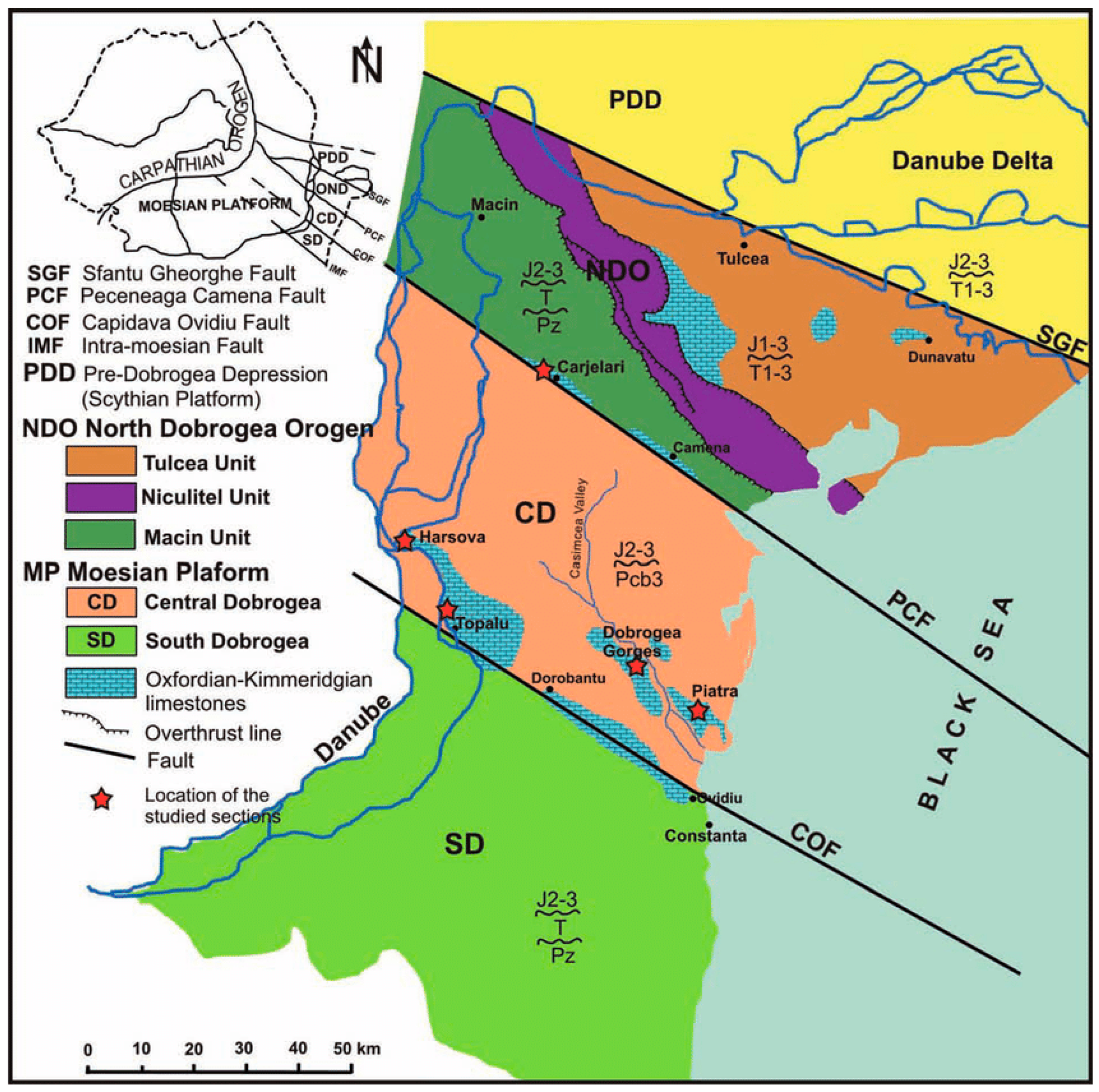
Our study area comprises the Casimcea catchment situated on the Back Sea littoral (Figure 1). From a geological point of view, the Casimcea basin is located in the Casimcea Plateau, the oldest geological unit in the Black Sea basin [23], situated between Peceneaga–Camena (FPC) and Capidava–Ovidiu (FCO) faults (Figure 2). The Casimcea Valley is cut into formations of green schists that emerge at the surface in several areas. Along the valley, there are sections of basins and gorges (particularly in the middle sector). In contrast, the valley has a canyon-like appearance in the lower sector, deeply cut into limestone.
The relief of the Casimcea basin decreases from an altitude of 300–350 m to a few meters, descending in steps toward Lake Tasaul (Figure 1). The mean elevation of the basin is 309 m, with an average slope of 4%. From a climatic point of view, the area falls under a temperate continental climate. The average temperature is around 11.2 °C [19], and the mean precipitation is 400 mm/yr [24].
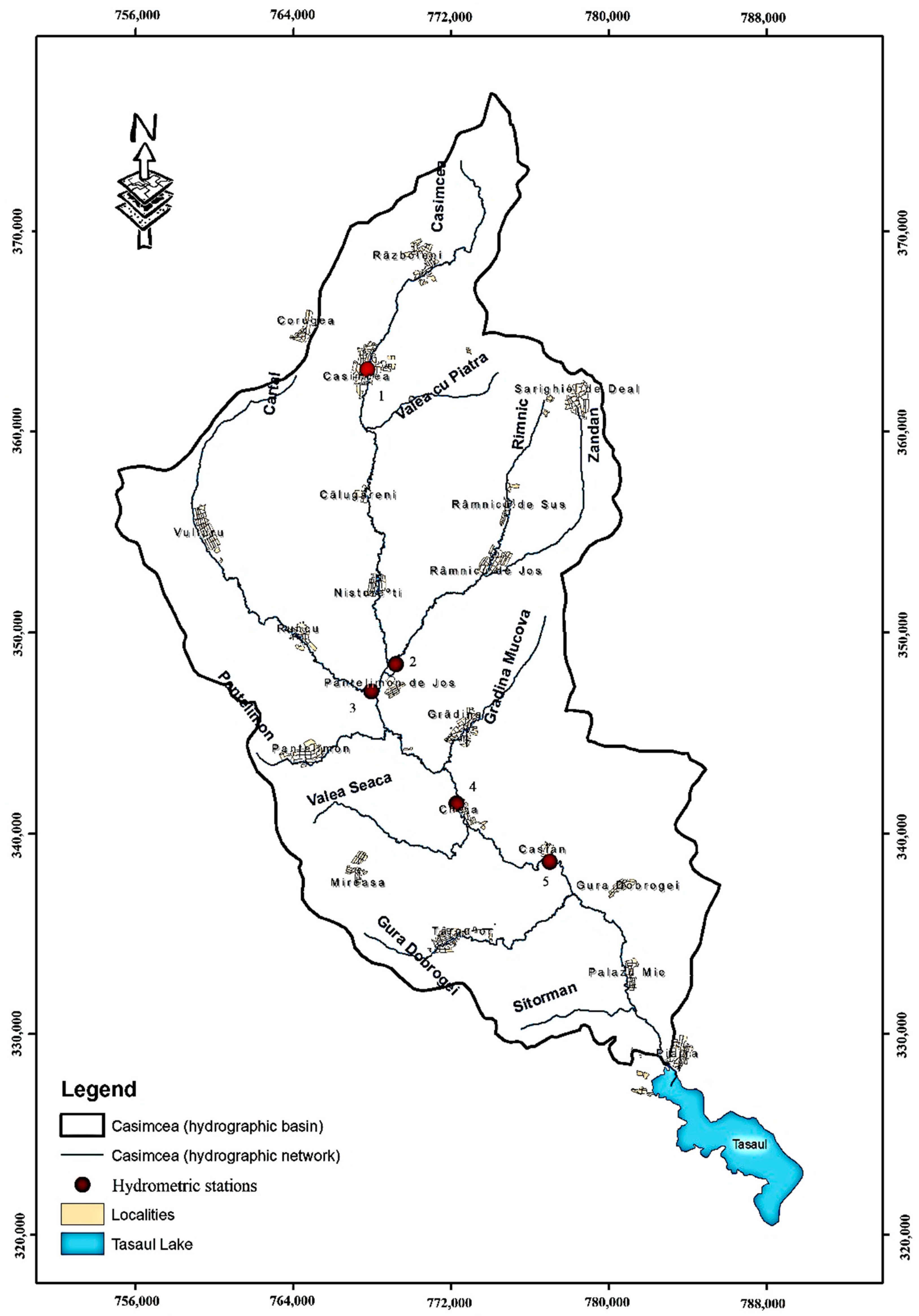
The Casimcea catchment (surface = 740 km2, length = 69 km) is drained by the river with the same name. The Casimcea River originates in the Casimcea Plateau and flows into Lake Taşaul. The Casimcea River has multiple tributaries, mostly on its right bank, including Cartal or Dereaua Mare, Pantelimon, Valea Seacă, and Gura Dobrogei. Râmnic, Grădina, and Mucova are the tributaries on the left side (Figure 3). The multiannual mean discharge is 0.630 m3/s. Dobrogea’s hydrology is distinguished by its low surface runoff and torrential hydrological regime, which comes from the unequal distribution of precipitation [25].
Figure 2. Simplified geological map of Dobrogea [26].
Hydrology 12 00172 g002
The Casimcea River crosses a limestone hilly area [27]. Between Cheia village and Lake Taşaul (Figure 3), an area of Oxfordian–Kimmeridgian carbonate deposits is well-known as Jurassic limestone, where water circulates only through voids and fissures [26]. From these limestone formations, a strong spring originates near Piatra village, known as “Izvorul Turcului” (Turks Spring) [25], which could not influence the discharge of the Casimcea River because it is close to Lake Tasaul (see Figure 3). To conclude, precipitation and limestone formation particularly influence the flow regime of the Casimcea River and its tributaries.

2.2. Materials and Methods

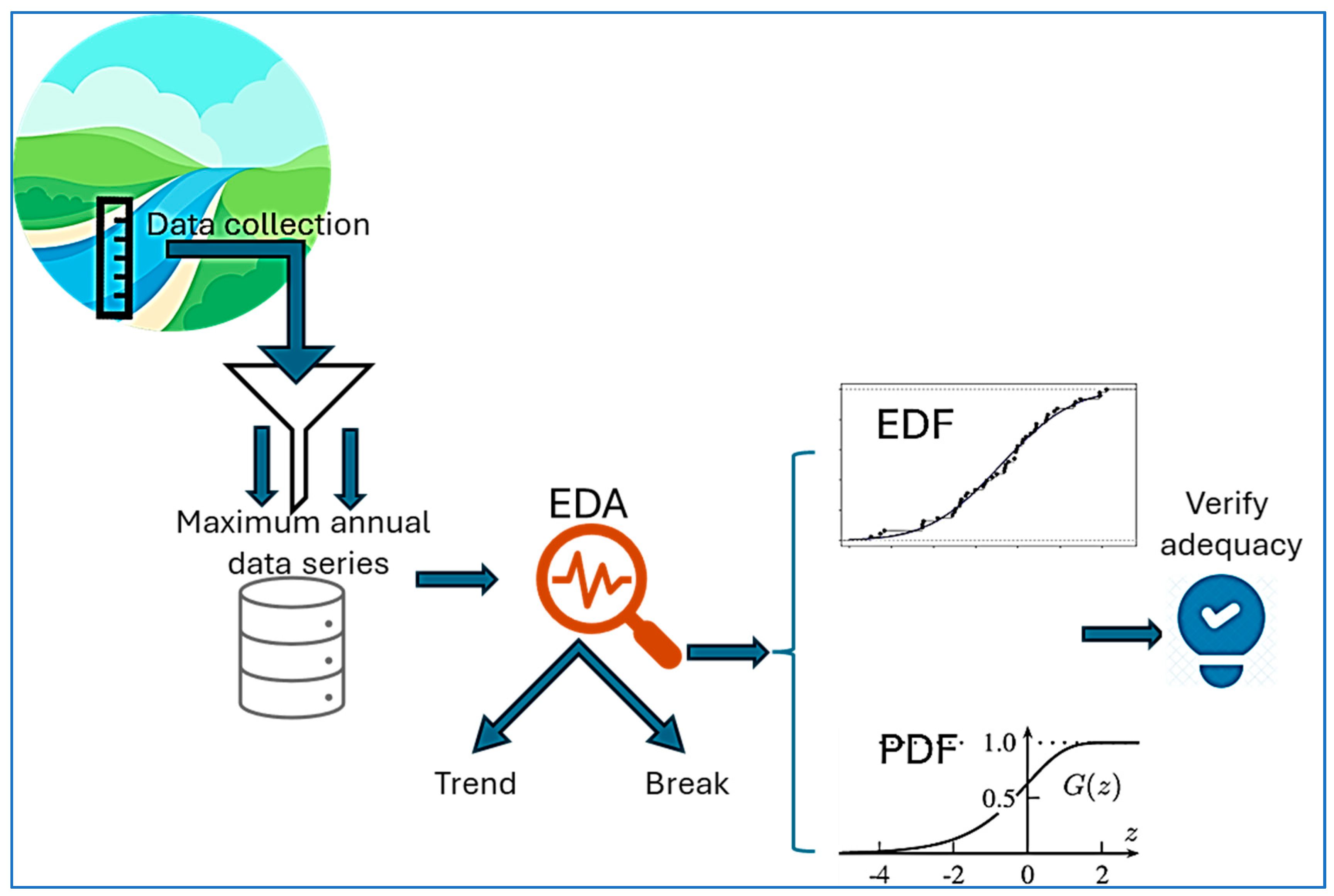
The methodology proposed in this paper is presented in Figure 4. The data were obtained from the National Agency for Water of Romania (NAWR). Detailed information about datasets is available in Section 2. After establishing the time series of maximum discharges, a series of methods were applied, consisting of Exploratory Data Analysis (EDA) and the identification of the empirical distribution function (EDF) and the theoretical probability distribution functions (PDFs). The EDA method consists of trend and break analyses.
The maximum discharge values estimated through PDF are compared with those observed and described through EDF using a series of error coefficients. Section 2.3 provides a detailed description of the methods used.

2.3. Data Collection

We used the datasets from the NAWR. In the Casimcea hydrographic area, there are four hydrometric stations, two on the main course (Casimcea-1 and Cheia-4 stations; see Figure 3), and two placed on the most important tributaries of the Casimcea River, located on the watercourses of Cartal (2) and Râmnic (3) (Figure 3). The Cheia hydrometric station (4) was installed in 1988 on the lower course of the Casimcea River, approximately 100 m upstream of the locality Cheia, in Constanța County. Before this date, the hydrometric station operated near the locality of Casian, approximately 5 km downstream from Cheia station.
The data were obtained from the National Agency for Water of Romania (NAWR); therefore, it is expected that they should be accurate and free from errors. Two sets of data series were collected: (i) annual maximum discharge (1965–1991) and (ii) maximum monthly discharge rate (the period 1992–2021). Based on monthly maximum time series data over the 1992–2021 period, we extracted the annual maximum discharge and created an annual maxima dataset for each hydrometric station.

3. Analytical Methods

Frequency analysis is a statistical method of prediction used to interpret past events and characteristics of a given process (hydrological or of a different nature) and to define the probabilities of occurrence for certain given values in the future. Prediction involves defining and introducing a frequency model, which is a mathematical equation that describes the statistical behavior of a random variable through its probability distribution function [27]. Such a method involves going through several stages, among which we mention (i) choosing the data series (according to the defined purpose), (ii) control of the data series, (iii) choosing the frequency model, (iv) calibrating the frequency model, and (v) validating the frequency model.
In line with the methodology proposed (Figure 4), EDA (Exploratory Data Analysis) was used. Special attention should be given to the distributional changes in time in the time series. Kundzewicz and Robsson [28] consider that a “modification” in the time series can be “monotonic,” represented by either a trend (increasing or decreasing) or an abrupt change, i.e., a breakpoint.
To verify the presence of a trend in the time series data, the Mann–Kendall test [29] was used. The null hypothesis, H0, states that there is no trend (i.e., no change in the mean), while the alternative hypothesis, H1, states that the mean of the series is either increasing or decreasing. The slope estimation was achieved using the non-parametric method called Sen’s method, implemented via MAKESENS (v 1.0) software. A break is often characterized as a sudden shift in the probability law of the time series at a specific period, which is normally unknown. The presence of breakpoints in the time series data was verified using Khronostat software (v 1.0). Several statistical tests to detect breaks are available within this software, such as Pettitt [30], Buishand [31], Lee & Heghinian [32], and Hubert [33]. According to these tests, the null hypothesis is tested, i.e., “no break in the series”.
According to the methodology proposed (Figure 4), the empirical distribution function (EDF) was used, along with Hydrognomon [34] software (v 4), to identify the theoretical probability distribution function (PDFs) model. Hydrognomon is an open-source software tool created to analyze hydrological data. According to [34], Hydrognomon software can offer advanced statistical analysis of hydrological datasets, including sample statistics, parameter distributions of several PDF models, such as the EV, log-normal distribution, and Gamma families, statistical prediction, and more. Once the theoretical model is chosen, it must be subjected to a series of tests to verify its adequacy for the sample used. Hydrognomon has only two tests to confirm the adequacy of PDFs: the Kolmogorov–Smirnov (KS) test and the Chi-Square test. The Kolmogorov–Smirnov (K-S) test is implemented in Hydrognomon software as a goodness-of-fit statistical test that verifies whether a sample belongs to a particular population distribution. According to the user manual [35], the K-S test assesses the most significant deviation between the theoretical and empirical distribution functions using the following equation:
D i = | F 0 ( x i ) F ( x i ) | ,
where F 0 is the empirical, and F is the theoretical distribution function. The Dmax parameter is set as the maximum Di, which is compared with the critical value Dcr, based on the specified significance level α.
If D m a x D c r then the null hypothesis is rejected. Computationally, this approach is reversed: given Dmax of the sample and the fitted theoretical distribution function, the K-S significance level αD is calculated. If the computed αD is smaller than the chosen significance level α, the null hypothesis H0: “The theoretical distribution function that hypothetically coincides with the real distribution function for every point j of the sample xj” [35] is rejected. The significance level, αD, is calculated using the following equation:
a D = 1 L ( z ) ,
where
L z = 2 π z k = 1 e 2 k 1 π z 8 ,     i f   0.3 z 8.5 L z = 0 , i f   z < 0.3 , L ( z ) = 1 ,   i f   z > 8.5 ,
z = D n m a x ,
n is the sample size, and c is a correction coefficient introduced if n < 50 ,
c = 0 , n 50 50 n 500 , n < 50 ,
In hydrology, the EDF is usually used to compute the flow duration curve, which represents the empirical cumulative discharge frequency as a function of the exceedance probability. The best-known equations for exceedance probability are presented in the table below (Table 1).
A probability plot is used to assess how well the data series follows a given probability distribution [36]. Finally, the maximum discharge values estimated through the PDF are compared with those observed and described through the empirical distribution functions. Pearson correlation coefficient (r), RMSE (Root Mean Squared Error), NSE (the Nash–Sutcliffe efficiency coefficient), and R2 (R-squared) are used to measure the performance of PDF models. It should be mentioned that the correlation coefficient (r) measures the degree of linear relation between the observed and predicted values. The range of variation of this coefficient is [−1; +1]. The degree to which the two time series are linearly correlated increases as the value of the coefficient reaches 1. The range of variation of R2 is between 0 and 1; the optimal value is 1. The Nash–Sutcliffe coefficient covers a scale from negative infinity to 1.0. A score below 0.0 denotes that the observed average makes better predictions than the model does, while a value of 1.0 denotes a perfect fit between the model and the observed data. The RMSE represents the standard error and varies within the range (0, + ); the optimal value is zero (0). A reduced RMSE suggests improved performance. The RMSE is susceptible to outliers and can be influenced by extreme values [37]. According to [38] “RMSE values less than half the standard deviation of the observation can be considered low”. For this reason, the ratio of the RMSE to the standard deviation of the measured data was calculated, following the recommendation of Singh [38].
Since we expect to obtain multiple PDF models for each river at specific hydrometric stations, and we will use five error indices as criteria for determining the model’s performance against measured data, we will use a multi-criteria decision analysis method. The ELECTRE (ELimination and Choice Expressing REality) method was chosen. An overview related to the ELECTRE method is presented in [39,40,41,42]. We just want to outline the main steps of the solution method: (i) developing the decision matrix, (ii) normalizing the decision matrix, (iii) computing the weighted normalized decision matrix, (iv) preparing the concordance and discordance sets, (v) calculating the concordance and discordance matrix, (vi) calculating the concordance/dominance and discordance index matrix, (vii) calculating the aggregate dominance matrix, and (viii) selecting the optimal variant.
Supporting decision-making is a key purpose of the models used. Confidence and prediction intervals for 95% are provided. By accurately measuring the uncertainty around these predictions, they provide valuable insights that enhance decision-making and bolster confidence in statistical analyses [43]. The confidence interval of the PDF selected is calculated through the Monte Carlo simulation process.

4. Results and Discussion

4.1. Floods Inventory

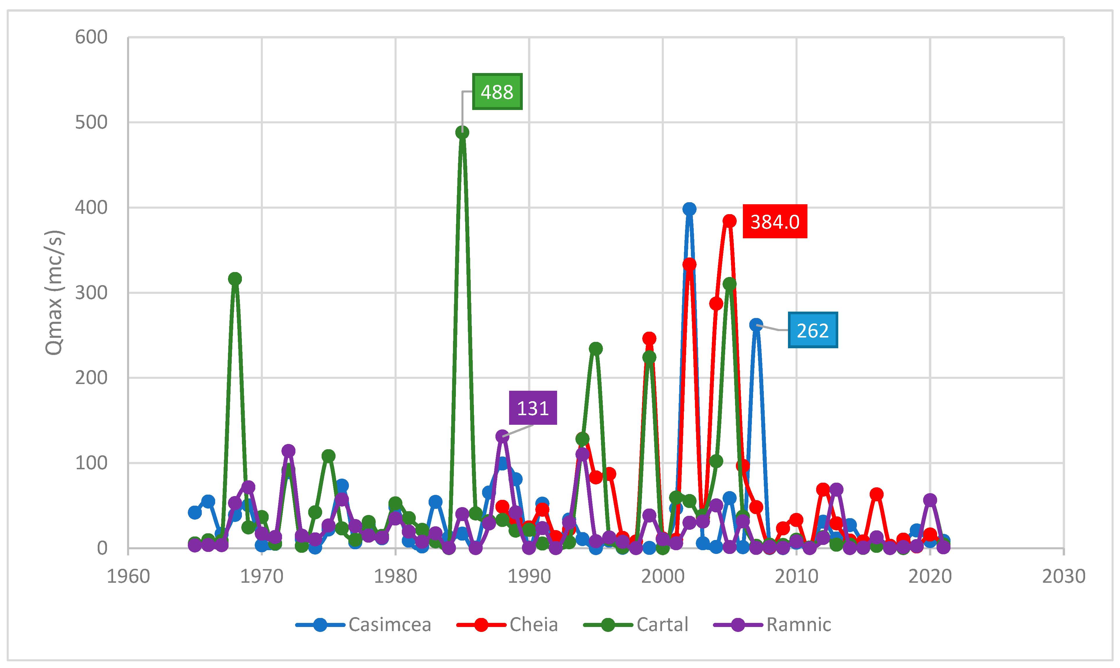
Table 2 presents geographical and hydrological information. Figure 5 shows the variation in annual maximum discharges for all hydrometric stations.
The discharge data have been measured since 1965 (57 years) for the Casimcea, Cartal, and Râmnic hydrometric stations and since 1988 (34 years), respectively, for the Cheia hydrometric station. We observed peak discharge values of 488 m3/s at the Cartal hydrometric station in 1985 (Table 2). At all the hydrometric stations under investigation, it has been noted that the maximum average discharge value exceeded the threshold between 1994 and 2007. It is noteworthy that at the Cartal station, in 1968 and 1985, discharges were recorded that exceeded the average value by 6-fold and 9-fold, respectively. The evolution of the time series data shows a similar pattern, with some exceptions: in 1968 and 1985, the Cartal hydrometric stations recorded two peak discharge values (316 m3/s and 488 m3/s, respectively), while all other rivers recorded values below 100 m3/s. Unfortunately, in the period 1965–1991, the Cheia hydrometric station was not yet installed, so we could not compare the values. The second anomaly occurred in 2002 at the Cheia hydrometric station, which recorded a discharge value of 333 m3/s, while the values registered at all other hydrometric stations ranged between 29 and 52 m3/s. In 2005 and 2007, the discharge values registered at the Cartal and Casimcea hydrometric stations, respectively, were 310 m3/s and 262 m3/s, respectively, while at the Cheia station, the discharge values were 24 m3/s and 48.1 m3/s. A flood inventory summary is provided in Table 3.
Based on the analysis of the recorded floods presented in the previous paragraphs, we could consider those values to be outliers, or the geology of the study area and precipitation could influence the discharge values. NAWR considers all those values as estimated historical events; large flood peaks are rarely directly observed. As can be observed, the annual floods, characterized by the highest yearly maximum discharge, occur most frequently in June and July [41]. In contrast, floods are the least frequent between October and April. The leading cause of these floods is the large amount of precipitation that falls in less than 24 h (in 2005, 73 mm and 24 mm of precipitation were recorded in less than 3 h and 30 min, respectively, at the Casimcea and Cartal stations). Unfortunately, we do not have enough data about the damage caused. However, in 2002, the estimated damage was RON 1268 million. The following paragraphs present an inventory of historical floods recorded in the Casimcea River basin [18,42,43,44].

4.2. Frequency Analysis Results

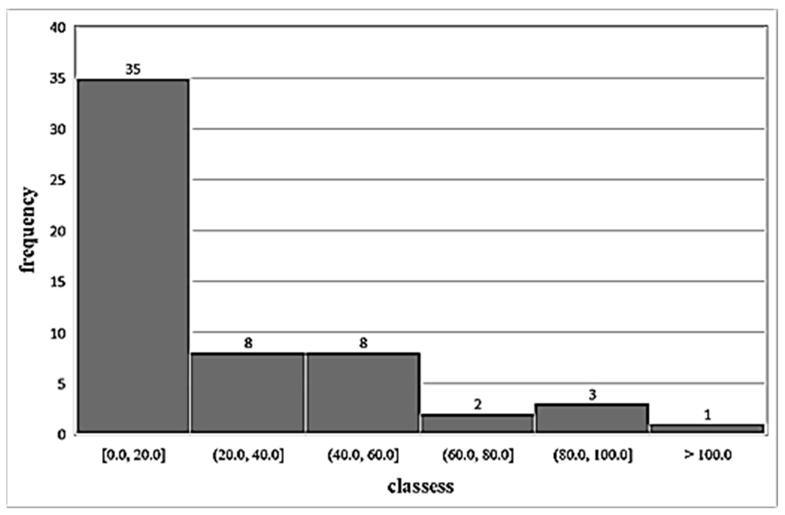
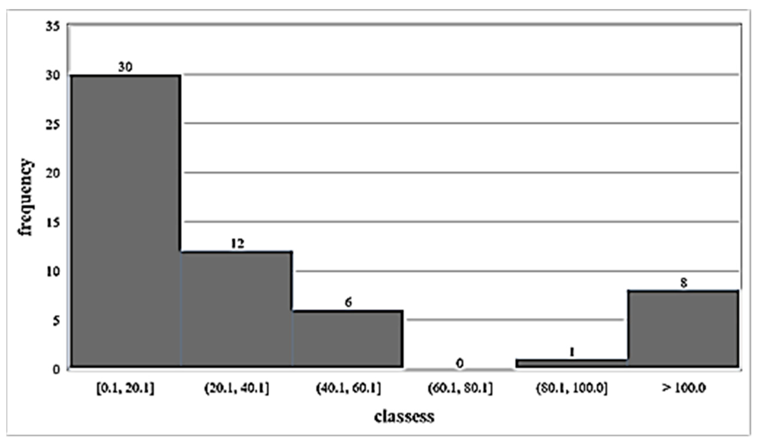
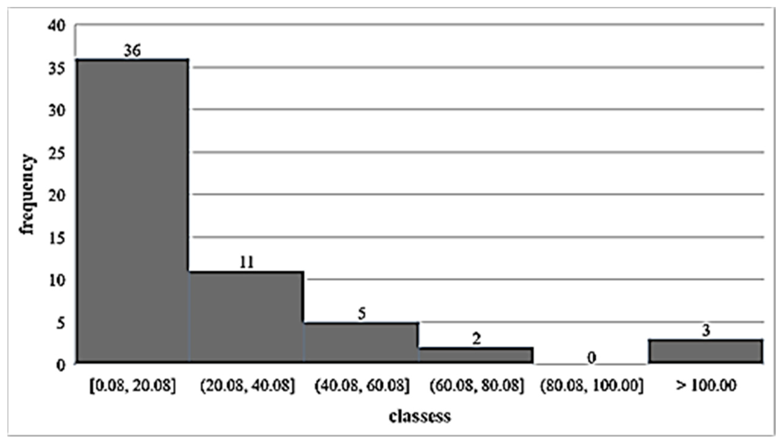
Figure 6, Figure 7, Figure 8 and Figure 9 present the histograms for each hydrometric station. All histograms are skewed to the right, with most of the events occurring in the range of 0–20 m3/s (between 41%—Cheia station and 61%—Râmnic station). Hydrological events with very high discharges, exceeding 100 m3/s, vary from station to station: at Casimcea and Râmnic hydrometric stations, there was only one such event and three events, respectively, representing less than 5% of the total. However, at the other two stations (Cheia and Cartal), these events account for just over 12% of the total. Based on the descriptions provided in the paragraphs above, the most suitable theoretical distribution functions for these events could be from the Weibull and log-normal families.
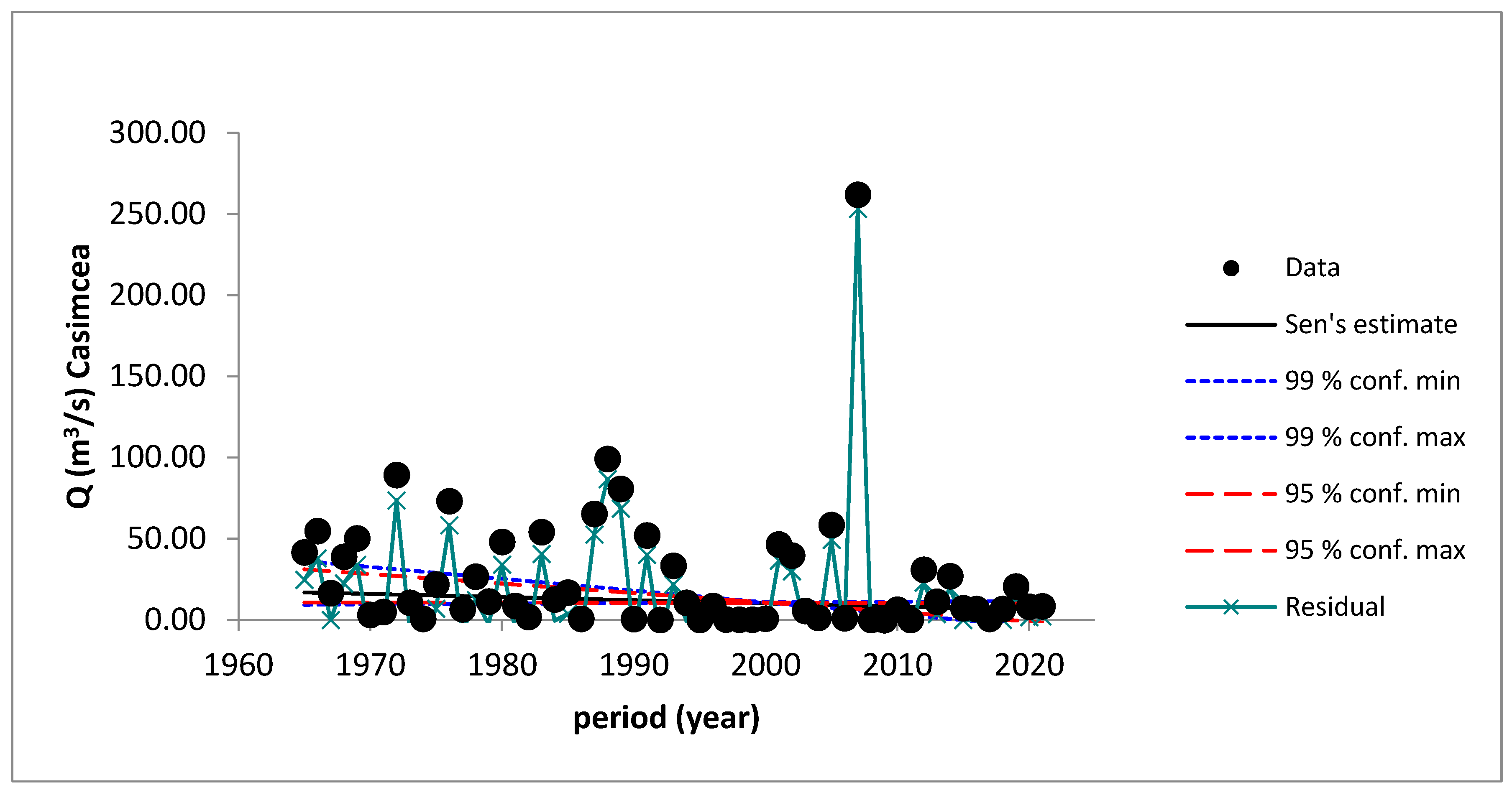
As we mentioned in the methods and methodology section, we investigated trends and breakpoints in time series data. Let us also remember that MAKESENS software is used to detect trends, and Khronostat software detects a breakpoint. Four significance levels (a) are tested by MAKESENS software: 0.001, 0.01, 0.05, and 0.1. In Table 4, the results obtained from the Mann–Kendall test are presented. We can see that the Z statistics are negative, and the slopes estimated are negative and vary between −0.194 and −0.908 (Table 4). These results indicate that the annual maximum discharge decreases for all stations investigated, at a 0.05 significance level. Sen’s slope provides a negative slope, which is also demonstrated by the non-random residuals (Figure 10).
All of the time series investigated exhibit similar behavior (Table 4). Nevertheless, the statistical approaches might be applied independently to the decreasing and increasing subseries. In Table 5, we present the results of the statistical tests available within Khronostat software. Khronostat software offers a feature for testing the independence of the time series investigated. The independence test is used to assess the possibility that no relationship exists among the variables within a population, based on a sample [45]. The software uses the rank correlation test. The null hypothesis tested was H0: “the series contain realization of independent random variables”. It must be mentioned that the Buishand [31] and the Lee & Heghinian [32] tests are procedures that are applied if the studied series is normally distributed. If the series is not normal, then different transformations are applied (such as a logarithm or a Box–Cox transformation) to normalize it. It should be noted that the Pettitt, Lee & Heghinian, and Hubert tests also provide the year in which the break in the time series data occurred.
The results show (Table 5) that the investigated time series are not random at the 95% confidence (significance levels of 0.1 and 0.05) and could suggest a trend or periodicity. An analysis of Table 5 shows that the Buishard, Pettitt, and Lee & Heghinian tests reject the null hypothesis at the significance level of 0.05 for the Casimcea, Cheia, and Cartal stations and at the significance level of 0.1 for the Râmnic hydrometric station. Hubert’s tests failed to reject the null hypothesis. Two of the three tests that could identify the year of a break indicate a change in 2006 for the Cartal and Ramnic stations, 2007 for the Cheia station, and 1989 for the Casimcea hydrometric station. The investigated discharge data series is obviously not homogenous. According to the Lee & Heghinian test, the break is more severe at the Cheia station (0.4131 break point probability) compared to the Casimcea (0.0738 break point probability), Cartal (0.1616 break point probability), and Râmnic (0.1175 break point probability) stations.
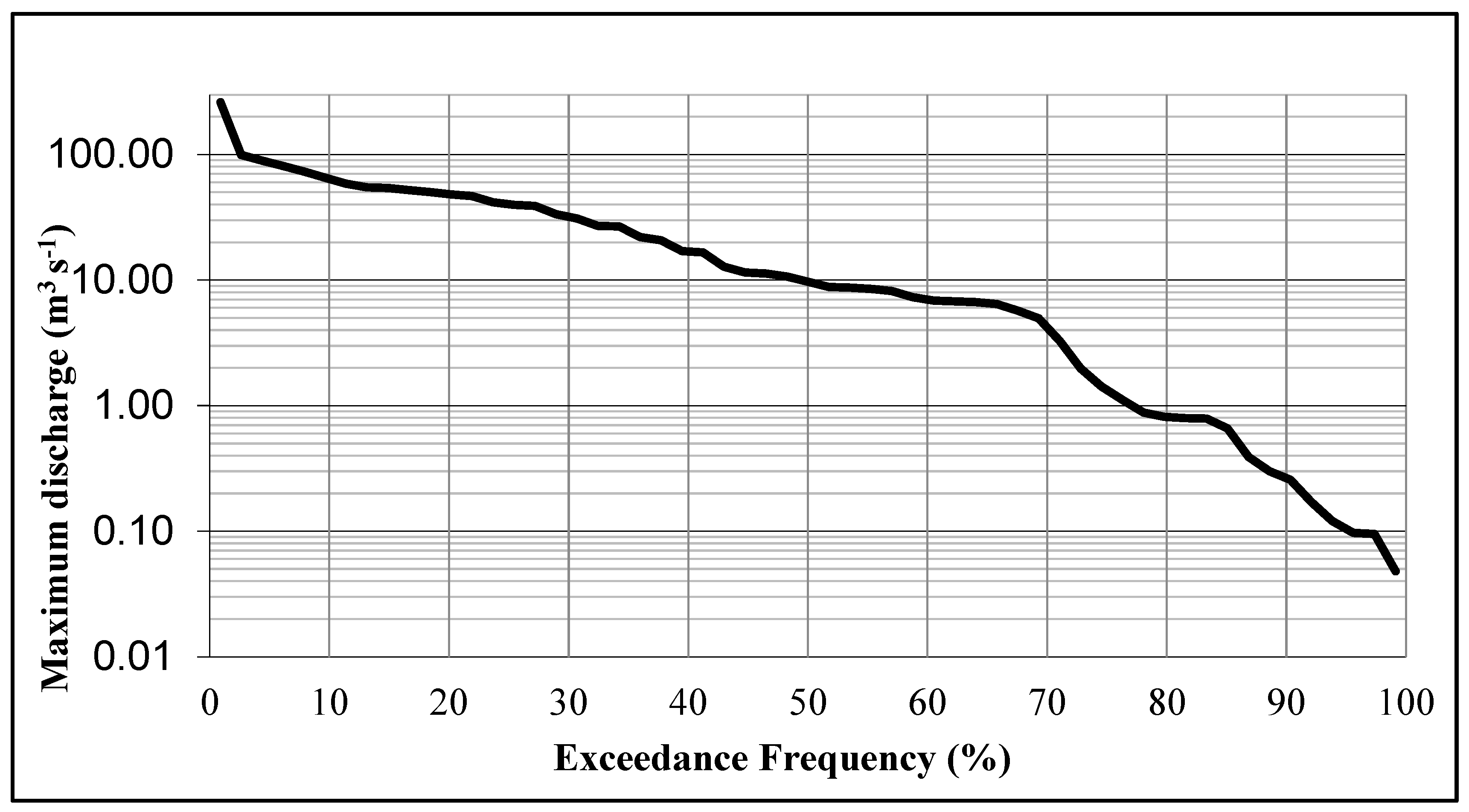
The flow duration curve (FDC) was determined using two empirical cumulative frequency functions: Hazen and Weibull. The flow duration curves for all hydrometric stations were plotted using Excel. Figure 11 presents an example of an FDC estimated through the Hazen equation for the Casimcea River at the Casimcea hydrometric station. The maximum discharge corresponding to different exceedance probabilities was extracted.
Generally, there are significant regional variations in the FDC shapes. According to a study by Ma [46], FDCs display an “L-shape” in the Americas and an “S-shape” in North China and differ from basin to basin. For the Casimcea basin, the FDC shape has an “S-shape”, but the last part of the S-shape, between 90 and 100 exceedance probability, is not well defined. In addition, in the final third of the curve, we observed (Figure 11) a steep slope which corresponds to a highly variable stream that receives most of its flow from direct runoff.
The values obtained from the PDFs were compared with those extracted for 100, 50, 20, 10, 5, and 2 return periods, as calculated using the Hazen and Weibull equation (Table 6). The Weibull equation could not calculate the discharge value for a 100-year return period (1% probability of exceedance) for the Cheia hydrometric station because the time series data have only 34 values.
Using Hydrognomon [34] software, we investigated the best theoretical probability distribution functions (PDFs) that could be applied to the time series data. The results for the Casimcea hydrometric station are presented in the table below (Table 7) (only the accepted PDFs for all levels of significance).
In Table 7, “a” represents the level of significance, and Dmax represents the maximum of the difference between the theoretical and the empirical distribution functions [35]. The goodness-of-fit test used was the Kolmogorov–Smirnov test. Furthermore, Hydrognomon includes only two tests to verify the adequacy of PDFs: the Kolmogorov–Smirnov (KS) test and the Chi-Square test. According to the KS test, the Dmax was sequenced in ascending order, from 1 to 7. Accordingly, the accepted distribution functions for all hydrometric stations are presented in Table 8. As can be observed in Table 8, not all individual accepted probability distribution functions are valid for all stations. For example, the Pearson-III distribution function is valid only for the Casimcea hydrometric stations (Table 8). GEV-Min yields good results only for the Casimcea hydrometric station (rank 3). The Pareto PDFs produced the same results as GEV-Min.
Koutsoyiannis noted in [20] that Jenkinson (1955) considers the EV3 distribution as “the most frequently found in nature since it is reasonable to expect the maximum values to have an upper bound”. Jenkinson mentioned that EV type 3 is limited in the direction of the extreme values [47]. The method of moments is frequently used to calculate the parameters of probability distribution functions. However, this method could have some disadvantages: (i) difficulty in assessing the shape of a distribution, (ii) the moment values can differ significantly from those of the probability distribution if the sample is small, and (iii) the calculated parameters are frequently less accurate. Applying an alternative approach, called L-moments (LMOs), could solve the previously mentioned limitations [48]. In this context, we decided to use only the PDFs valid for all hydrometric stations: Gamma, EV3-Min (Weibull), Pareto, and GEV-Min. The results provided by PDFs indicate the following: (i) the maximum discharge value for 100-year return periods (Table 9) is underestimated; (ii) the values predicted for 10, 5, and 2-year return periods have a good estimation using all five PDFs used. Similarly, maximum discharge values for each hydrometric station were calculated. The same behavior was observed. However, the most important conclusion is that the models cannot be chosen based solely on the value obtained for the rank value. This is why we used a series of coefficients that determine the error between the modeled and observed values. The maximum discharge values for the following return periods (1000, 100, 50, 20, 10, 5, and 2 years) were initially determined before computing the error indices. The values of maximum discharge for the Casimcea hydrometric station, estimated using the chosen PDFs and the EDF values corresponding to the return period are presented in Table 9. Similarly, values were established for all hydrometric stations along the river and its tributaries.
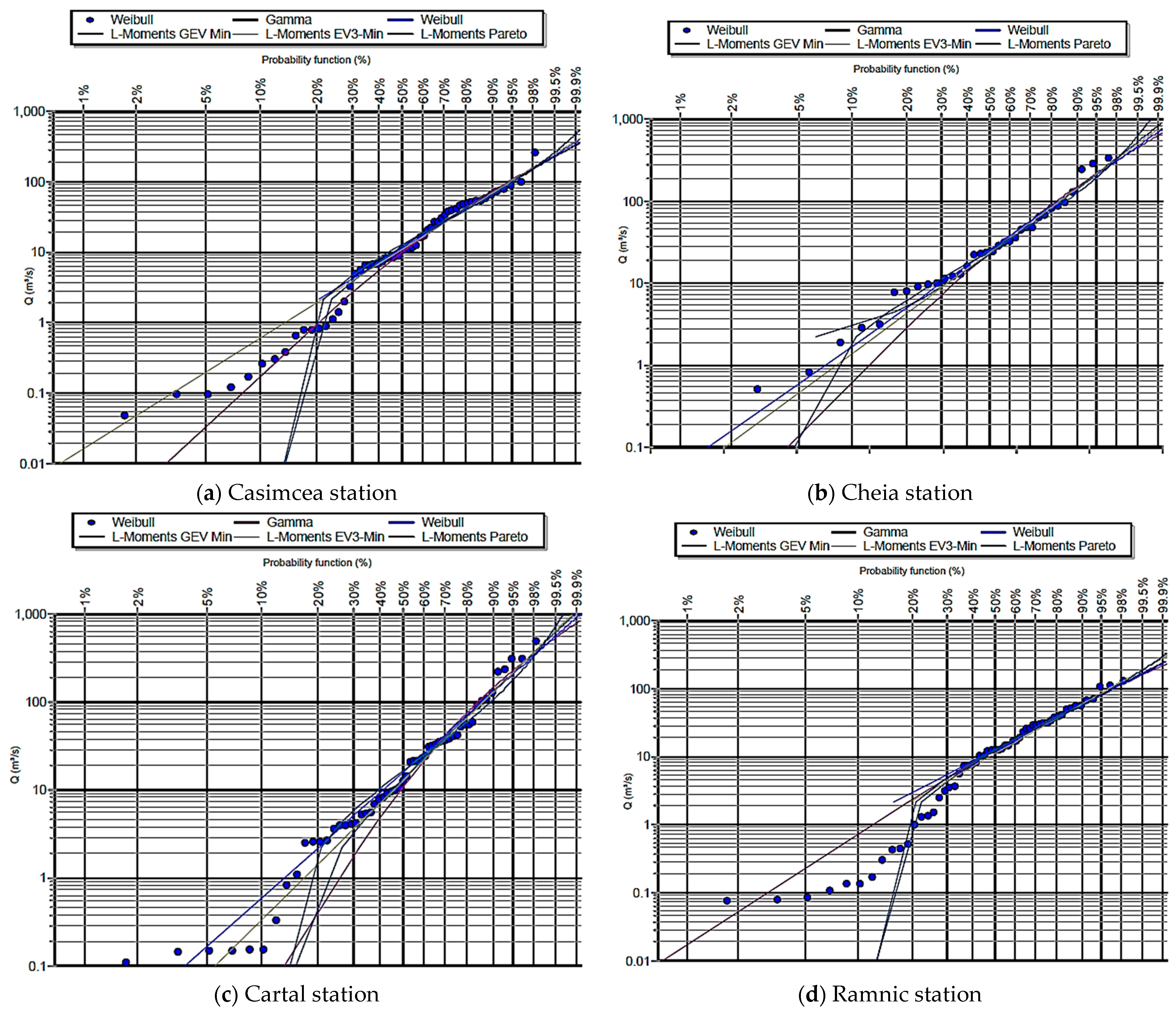
The results of the probability plots for all stations were created and presented in the following figures.
Only the first five selected PDFs (according to Table 10) were plotted. As can be seen from Figure 12, the Gamma and EV3-Min (L-moments) functions manage to simulate the data quite well. Figure 12 shows that the distribution of EV3-Min (L-moments) aligns closely with the data, especially with the right tail; the left tail is overestimated. Pareto (L-moments) and GEV-Min (L-moments) functions offer a good simulation only for the data situated between 30% and 99%; for the rest (especially in the right tail), the two functions overestimate the data. Exceptions were found only for the flow registered at the Cartal and Cheia stations, where the two distribution functions also offer good results for the 20–30% range.

4.3. Results of Adequacy Tests

The maximum discharge values estimated through PDF are compared with the value observed through the empirical distribution functions using several indices mentioned in the methodology section. The results are provided in Table 10.
The results presented in Table 10 show the following: (i) The r coefficients yield good values, close to 1, which means an excellent correlation between observed and modeled values; however, there are several exceptions: at the Râmnic station, the r values range between 0.79 and 0.87, so we can conclude that a strong positive linear relationship exists between observed and modeled maximum discharges values. (ii) R2 also yields good results for the Casimcea station but for the other stations, the R2 values are over 0.85; an R2 > 0.5 is usually considered as satisfactory. (iii) The NSE produces values close to zero or negative; an NSE value close to zero indicates that the model estimates are as accurate as using the mean of the observed data, while a negative NSE value indicates that the models used fail to reproduce the mean, which indicates unacceptable performance. (iv) The RMSE values must be interpreted carefully. The RMSE falls within the interval of 25.68 m3/s to 172.03 m3/s. The PDF models with the lowest RMSE values achieved the best results. The RMSE uses the same units as the dependent variable (m3/s), and it is sensitive to outliers.
The results obtained by applying the error functions, presented in Table 10, are similar to those obtained by probability plots. A limitation of the results derived from the methodology is the reliance on the KS test, which has a well-documented tendency to exhibit lower power in assessing goodness-of-fit [39]. However, the application of the Anderson–Darling test did not show a significant difference in goodness-of-fit evaluation. To ensure continuity in this study, we made a deliberate decision to consistently utilize the results of the KS test.

4.4. Results of the ELECTRE Method

In line with the results presented in Table 10, it is difficult to choose the best-performing PDFs. For this reason, the best PDF model was selected using the ELECTRE method. According to this method, the criteria selected are rank, r coefficient, RSR (RMSE/STDEV), NSE, and R2. Based on a review published in 2007, Moriasi [49] established performance ratings for the NSE and RSR index. The criteria and values for each of them are presented in Table 11. The cells marked in green in Table 10 represent the best results according to Table 11.
Please note that for the r coefficient, NSE, and R2 error indices, the closer the obtained values are to 1, the better the model performance, whereas for RSR, lower values, tending toward zero, indicate better model performance. Accordingly, the r coefficient, NSE, and R2 criteria were maximized, indicating that a criterion’s priority increases with its score, whereas RSR was minimized. This implies that the lower the criterion score, the more desirable it is. In the process of assigning weights, values are allocated to the chosen criteria to indicate their relative significance. The criteria and weight are presented in Table 12. We consider assigning greater weight to the results obtained through the goodness of fit PDF (results obtained using Hydrognomon software). In this manner, all error indices were assigned equal weights, and the rank criterion was assigned a weight of 50%.
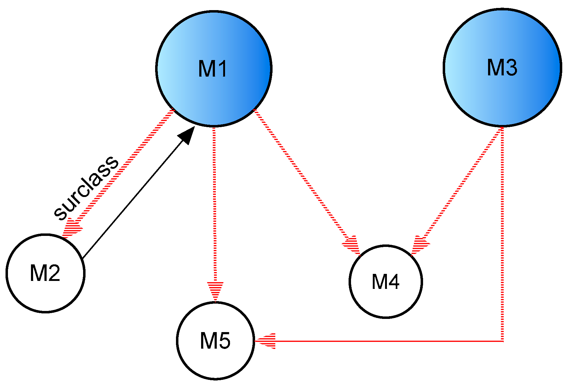
The models investigated are those presented in Table 10. These are denoted by M from 1 to 5 in the order given in Table 10 for each station. Selecting the optimal variant is based on the net superior and inferior values for each station. The results obtained are presented in Table 13. The computation of net superior/inferior results shows that M2 (EV3-Min-Weibull, L-moments) achieved the maximum value and M5 (GEV-Min-L-moments) the minimum value, and they have been assigned ranks 1 (the best scheme) and 5 (the poorest scheme), respectively. The computation of the net superior values shows that M1, M3, and M4 were assigned the ranks 3, 4, and 2. On the other hand, the M1, M3, and M4 models ranked third, fourth, and second, respectively, when the reliability design approach was ranked based on net inferior values. According to the ELECTRE method, M1, M3, and M4 are excluded (denoted by E in Table 13). There were some problems at the Râmnic station. The results obtained for the net superior and inferior values show that only the M5 model could be retained. In this case, EV3-Min-Weibull (L-moments) is the best PDF model for the Casimcea River at the Casimcea station and for the Cartal River at the Cartal station. GEV-Min-L-moments is the choice for the Casimcea River at the Cheia hydrometric station. For the Râmnic River at the Râmnic station, the favorable model is EV3-Min-Weibull. For this river, the model was assigned to the fifth rank. In this context, the aggregate dominance matrix was investigated. This matrix is presented in Table 14. According to [42], if at least one element “1” is present in a column, that column must be eliminated, which signifies that the related row(s) “are ‘ELECTRE-cally’ dominant over the column” [42]. That means that columns 1,2, 4, and 5 must be eliminated, and the model M3 is the favorable alternative (see also Table 13: the net superior value at the Râmnic station for M3 is assigned rank 1). To better illustrate the relationships in this phase, a graphical representation of the overall classification can be useful.
In the example for the Râmnic station (Figure 13), M2, M4, and M5 are dominated by M1 and M3, respectively. However, M1 is dominated by M2. The preference relationship between M1 and M3 could not be determined. This result could be obtained from the column of the aggregate dominance matrix (Table 14). M3 does not contain any element with a value of 1. According to the results presented in Figure 12, M3 (GEV-Min-L-moments) is the preferred choice, followed by M1 (Gamma).
Both risk analysis and the design process depend on the prediction interval and confidence interval, which play a crucial role in assessing the reliability of model predictors.
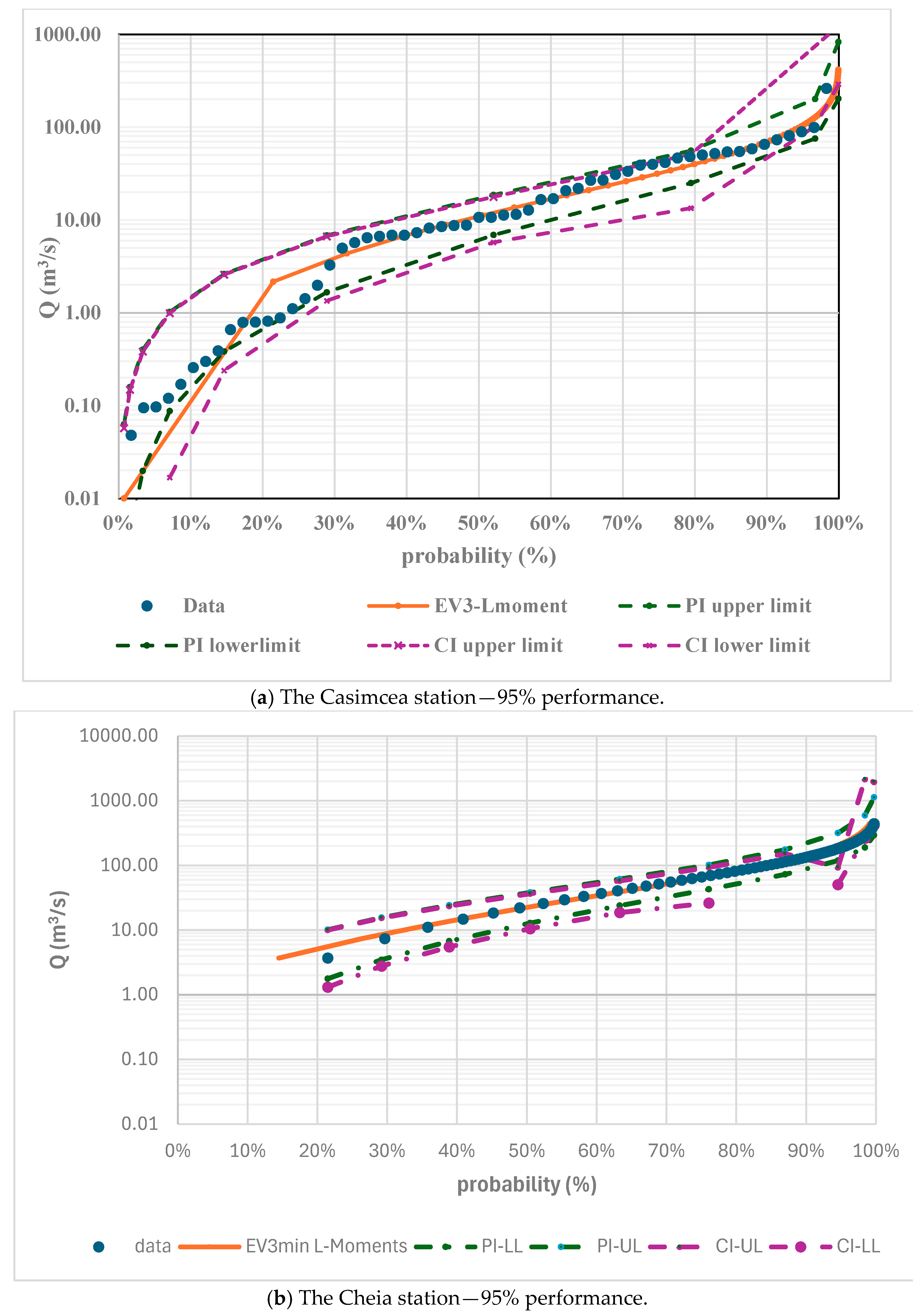
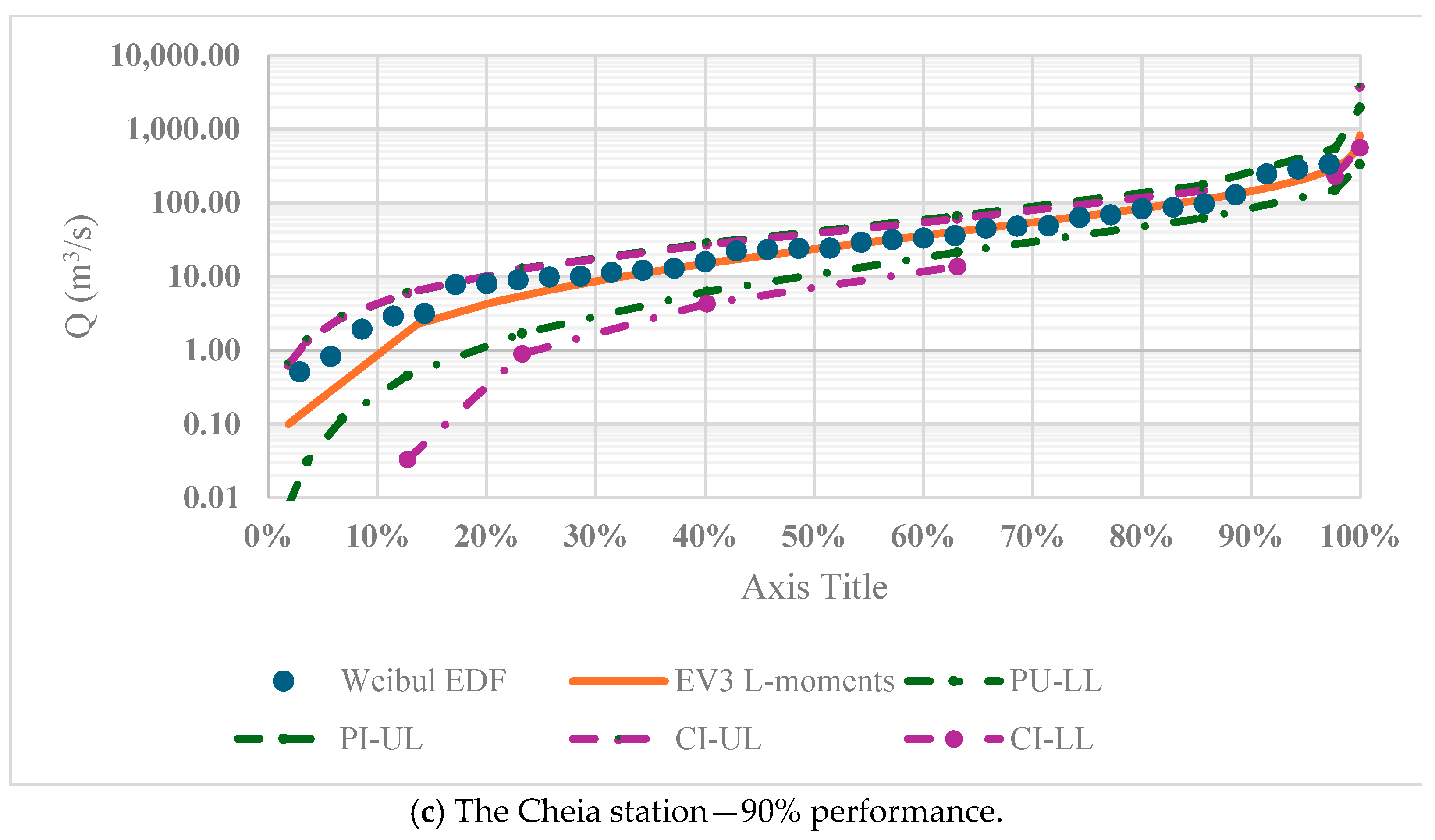
After applying the ELECTRE method, two cases were identified in the analysis of the CI results at 95% for the accepted function (Figure 14). The first one, related to the Casimcea station, shows that EV3-Min-Weibull (L-moments) function provides results within the CI limits. However, as expected, the left tail of the PDF falls outside of the PI interval, but it is within the CI intervals. The second case is related to the Cheia Station. At 95%, we identified an anomaly regarding the CI: the lower limit of CI (CI-LL) intersects the upper limit (CI-UL). We could consider the possibility that this anomaly may result from a size limitation or inaccuracy in determining the maximum values, which could affect the reliability of the confidence interval (CI). It is known that L-moments are particularly recommended when the tail of the distribution is quite dense and the sample size is small. In this case, the right tail of the distribution is not dense. The results obtained using EV3 Weibull show that it performs well (Figure 14c). We consider that it is difficult to recommend a single (optimal) PDF for all the rivers studied. A more advanced statistical analysis is needed, involving additional adequacy tests, such as the modified Anderson–Darling test. It is also important to explore other PDFs that are specially adapted for studying flow in arid regions.

5. Conclusions

This paper describes a study carried out to estimate maximum discharge values for the main river and its tributaries crossing the Casimcea catchment, using different PDF models. Empirical models cannot provide values for exceedance probabilities of 0.1%, 0.01%, or sometimes even 1%. Citing Kuczera, the authors of Bulletin 17C [50] argue that extensions of the exceedance curve can considerably affect the quantile estimates derived from such extrapolations. In this context, this study presented a suitable distribution using the goodness-of-fit measures provided by Hydrognom software and calculated by the Kolmogorov–Smirnov test. The suitable PDFs were classified according to their Dmax ranks. The observed and modeled values were compared using different error indices. As discussed in the previous paragraphs, it is difficult to interpret the results and choose the most favorable model. To improve the results, the ELECTRE method was chosen. The results of the ELECTRE analysis helped identify the best PDF model based on the criteria selected (error indices and corresponding ranks). In general, the model with the best rank score obtained using Hydrognomon software was not the one determined by the ELECTRE method. For example, at the Casimcea station, the best model obtained using Hydrognomon was Gamma. The ELECTRE method designated model EV3-Min (Weibull, L-moments) as the best one. This model showed better RSR, NSE, and R2 values than the Gamma model. The r coefficient yielded very similar results. The Gamma model was the third choice according to the ELECTRE results. To conclude, for the Casimcea River and its tributaries, a single PDF model cannot serve as a determinant, and hence a series of indicators, presented here, is necessary for predictive modeling. A limitation of this study is the extreme values recorded. It remains uncertain whether these are true values or just outliers caused by measurement methods (especially in the years before 2011, when automatic stations were introduced). A careful field analysis showed that the connecting roads crossing the Casimcea River (linking the left and right banks) are equipped with culverts that create obstacles because they have limited transport capacity. Water accumulates upstream of these culverts/bridges, the levels rise, and flood the adjacent territory. Due to the uncertainties in the data and the varying results, an event-by-event analysis using a numerical model should be employed to verify whether the gauge stations are providing accurate measurements and data.
Under climate change conditions, those designing flood-related infrastructure must pay attention to the factors that influence flow, such as geology and land use. The results of this study provide a foundation for creating detailed flood hazard and risk maps, which are essential for mitigating the impact of floods in Romania.

Author Contributions

C.M.: conceptualization, data curation, formal analysis, investigation, methodology, project administration, resources, software, supervision, validation, visualization, writing—original draft; C.C.: data curation, formal analysis, investigation, methodology, software, validation, visualization; A.V.: validation, visualization, writing—original draft, writing—review and editing. All authors have read and agreed to the published version of the manuscript.

Funding

This research did not receive any specific grant from funding agencies in the public, commercial, or not-for-profit sectors.

Institutional Review Board Statement

This study does not include human subjects, and no IRB approval was required.

Data Availability Statement

Most of the data reported is either contained in the document, available from the reporting stations, and/or easily available from the authors upon request.

Conflicts of Interest

The authors declare no conflicts of interest, financial or otherwise.

Jurisdictional Claims

No jurisdictional claim dispute is expected from this study. In addition, the authors have used their full, standard institutional names and addresses for independent verification for research integrity purposes.

References

  1. EEA. Climate Change, Impacts and Vulnerability in Europe 2012; European Environment Agency: Copenhagen, Denmark, 2012. [Google Scholar]
  2. Modeling and Monitoring Extreme Hydrometeorological Events; Maftei, C., Muntean, R., Vaseashta, A., Eds.; Advances in Environmental Engineering and Green Technologies; IGI Global: Hershey, PA, USA, 2023; ISBN 978-1-66848-771-6. [Google Scholar]
  3. The European Parliament. Directive; The European Parliament: Strasbourg, France, 2007; Volume 288. [Google Scholar]
  4. Hall, J.; Arheimer, B.; Aronica, G.T.; Bilibashi, A.; Boháč, M.; Bonacci, O.; Borga, M.; Burlando, P.; Castellarin, A.; Chirico, G.B.; et al. A European Flood Database: Facilitating Comprehensive Flood Research beyond Administrative Boundaries. Proc. IAHS 2015, 370, 89–95. [Google Scholar] [CrossRef]
  5. EEA. Flood Risks and Environmental Vulnerability—Exploring the Synergies Between Floodplain Restoration, Water Policies and Thematic Policies; European Environment Agency: Copenhagen, Denmark, 2016. [Google Scholar]
  6. Kundzewicz, Z.W.; Krysanova, V.; Dankers, R.; Hirabayashi, Y.; Kanae, S.; Hattermann, F.F.; Huang, S.; Milly, P.C.D.; Stoffel, M.; Driessen, P.P.J.; et al. Differences in Flood Hazard Projections in Europe—Their Causes and Consequences for Decision Making. Hydrol. Sci. J. 2017, 62, 1–14. [Google Scholar] [CrossRef]
  7. Alfieri, L.; Bisselink, B.; Dottori, F.; Naumann, G.; De Roo, A.; Salamon, P.; Wyser, K.; Feyen, L. Global Projections of River Flood Risk in a Warmer World: RIVER FLOOD RISK IN A WARMER WORLD. Earth’s Future 2017, 5, 171–182. [Google Scholar] [CrossRef]
  8. Statista. Deadliest Floods in Europe 2021. 2023. Available online: https://www.statista.com/statistics/1295966/deadliest-floods-in-europe/ (accessed on 2 August 2023).
  9. Kundzewicz, Z.W.; Pińskwar, I.; Brakenridge, G.R. Changes in River Flood Hazard in Europe: A Review. Hydrol. Res. 2017, 49, 294–302. [Google Scholar] [CrossRef]
  10. Paprotny, D.; Morales-Nápoles, O.; Jonkman, S.N. HANZE: A Pan-European Database of Exposure to Natural Hazards and Damaging Historical Floods since 1870. Earth Syst. Sci. Data 2018, 10, 565–581. [Google Scholar] [CrossRef]
  11. Maftei, C.; Papatheodorou, K. Flash Flood Prone Area Assessment Using Geomorphological and Hydraulic Model. J. Environ. Prot. Ecol. 2015, 16, 63–73. [Google Scholar]
  12. Maftei, C.; Papatheodorou, K. Mathematical Models Used for Hydrological Floodplain Modeling. In Extreme Weather and Impacts of Climate Change on Water Resources in the Dobrogea Region; IGI Global: Hershey, PA, USA, 2016; pp. 69–100. ISBN 978-1-4666-8438-6. [Google Scholar]
  13. Gumbel, E.J. On the Frequency Distribution of Extreme Values in Meteorological Data. Bull. Am. Meteorol. Soc. 1942, 3, 95–105. [Google Scholar] [CrossRef]
  14. Raynal, J.A.; Salas, J.D. Estimation Procedures for the Type-1 Extreme Value Distribution. J. Hydrol. 1986, 3–4, 315–336. [Google Scholar] [CrossRef]
  15. El Adlouni, S.; Bobée, B.; Ouarda, T.B.M.J. On the Tails of Extreme Event Distributions in Hydrology. J. Hydrol. 2008, 355, 16–33. [Google Scholar] [CrossRef]
  16. De Gusmão, F.R.S.; Ortega, E.M.M.; Cordeiro, G.M. The Generalized Inverse Weibull Distribution. Stat Pap. 2011, 52, 591–619. [Google Scholar] [CrossRef]
  17. Weibull, W. A Statistical Distribution Function of Wide Applicability. J. Appl. Mech. 1951, 18, 293–297. [Google Scholar] [CrossRef]
  18. Cerneagă, C.; Maftei, C. Flood Frequency Analysis of Casimcea River. IOP Conf. Ser. Mater. Sci. Eng. 2021, 1138, 012014. [Google Scholar] [CrossRef]
  19. Maftei, C.; Barbulescu, A. Statistical Analysis of Climate Evolution in Dobrudja Region. In Proceedings of the World Congress on Engineering, London, UK, 2–4 July 2008. [Google Scholar]
  20. Koutsoyiannis, D. Statistics of Extremes and Estimation of Extreme Rainfall: I. Theoretical Investigation/Statistiques de Valeurs Extrêmes et Estimation de Précipitations Extrêmes: I. Recherche Théorique. Hydrol. Sci. J. 2004, 49, 3. [Google Scholar] [CrossRef]
  21. Balkema, A.A.; De Haan, L. Residual Lifetime at Great Age. Ann. Probab. 1974, 2, 792–804. [Google Scholar] [CrossRef]
  22. Pickands, J. Statistical Inference Using Extreme Order Statistics. Ann. Stat. 1975, 3, 119–131. [Google Scholar]
  23. Berbecariu, A.; Vespremeanu-Stroe, A. In Search of Marine Terraces from Central Dobrogea (Casimcea Plateau, Western Black Sea). Preliminary Inquiries on Distribution, Extension and Vertical Crustal Movements. Rev. De Geomorfol. 2020, 22, 87–97. [Google Scholar] [CrossRef]
  24. Maftei, C.; Barbulescu, A. Statistical Analysis of Precipitation Time Series in Dobrudja Region. Mausam 2012, 63, 553–564. [Google Scholar] [CrossRef]
  25. Ciulache, S.; Torică, V. Clima Dobrogei (Dobrogea Climate). In Analele Universității București, Seria Geografie (Annals of the University of Bucharest – Geography Series); University of Bucharest: București, Romania, 2003; pp. 83–107. [Google Scholar]
  26. Schweitzer, C.E.; Lazăr, I.; Feldmann, R.M.; Stoica, M.; Frantescu, O. Decapoda (Anomura; Brachyura) from the Late Jurassic of Dobrogea, Romania. Neues Jahrb. Für Geol. Und Paläontol. Abh. 2017, 286, 207–228. [Google Scholar] [CrossRef]
  27. Meylan, P.; Musy, A. Hydrologie Fréquentielle; HGA: Bucureşti, Romania, 1999; ISBN 973-98954-5-X. [Google Scholar]
  28. Kundzewicz, Z.W.; Robson, A. Detecting Trend and Other Changes in Hydrological Data; WMO: Geneva, Switzerland, 2000. [Google Scholar]
  29. Zaiontz, C. Sen’s Slope Mann-Kendall Text; 2024.
  30. Pettitt, A.N. A Non-Parametric Approach to the Change-Point Problem. J. R. Stat. Society. Ser. C (Appl. Stat.) 1979, 28, 126–135. [Google Scholar] [CrossRef]
  31. Buishand, T.A. Tests for Detecting a Shift in the Mean of Hydrological Time Series. J. Hydrol. 1984, 73, 51–69. [Google Scholar] [CrossRef]
  32. Lee, A.F.S.; Heghinian, S.M. A Shift Of The Mean Level In A Sequence Of Independent Normal Random Variables—A Bayesian Approach. Technometrics 1977, 19, 503–506. [Google Scholar] [CrossRef]
  33. Hubert, P. The Segmentation Procedure as a Tool for Discrete Modeling of Hydrometeorological Regimes. Stoch. Environ. Res. Risk Assess. 2000, 14, 297–304. [Google Scholar] [CrossRef]
  34. Kozanis, S.; Christofides, A.; Mamassis, N.; Efstratiadis, A.; Koutsoyiannis, D. Hydrognomon—Open Source Software for the Analysis of Hydrological Data. In Proceedings of the European Geosciences Union General Assembly 2010, Vienna, Austria, 2 May 2010. [Google Scholar]
  35. Kozanis, S.; Christofides, A.; Efstratiadis, A. Scientific Documentation of the Hydrogram Software Version 4; Department of Water Resources and Environmental Engineering, National Technical University of Athens: Athens, Greece, 2010; p. 173. [Google Scholar]
  36. Das, S. Goodness-of-Fit Tests for Generalized Normal Distribution for Use in Hydrological Frequency Analysis. Pure Appl. Geophys. 2018, 175, 3605–3617. [Google Scholar] [CrossRef]
  37. Moriasi, D.; Gitau, M.; Pai, N.; Daggupati, P. Hydrologic and Water Quality Models: Performance Measures and Evaluation Criteria. Trans. ASABE (Am. Soc. Agric. Biol. Eng.) 2015, 58, 1763–1785. [Google Scholar] [CrossRef]
  38. Singh, J.; Knapp, H.; Arnold, J.; Misganaw, D. Hydrologic Modeling of the Iroquois River Watershed Using HSPF and SWAT. JAWRA J. Am. Water Resour. Assoc. 2005, 41, 343–360. [Google Scholar] [CrossRef]
  39. Abdolazimi, A.; Momeni, M.; Montazeri, M. Comparing ELECTRE and Linear Assignment Methods in Zoning Shahroud-Bastam Watershed for Artificial Recharge of Groundwater with GIS Technique. Mod. Appl. Sci. 2014, 9, p68. [Google Scholar] [CrossRef]
  40. Figueira, J.R.; Greco, S.; Roy, B.; Slowinski, R. Electre Methods: Main Features and Recent Developments. In Handbook of Multicriteria Analysis; Springer: Berlin/Heidelberg, Germany, 2010. [Google Scholar]
  41. Rosu, L.; Maftei, C.; Dobre, M.; Serban, A.; Iordache, G. ELECTRE Method Used in the Economical Analysis of Romanian Irrigation Systems; Bogazici University: Istanbul, Turkey, 2004; pp. 1358–1367. [Google Scholar]
  42. Taherdoost, H.; Madanchian, M. A Comprehensive Overview of the ELECTRE Method in Multi Criteria Decision-Making. J. Manag. Sci. Eng. Res. 2023, 6, 5–16. [Google Scholar] [CrossRef]
  43. Das, S. An Assessment of Using Subsampling Method in Selection of a Flood Frequency Distribution. Stoch. Environ. Res. Risk Assess. 2017, 31, 2033–2045. [Google Scholar] [CrossRef]
  44. Telteu, C.-E.; Stan, F.-I.; Brănescu, E.; Berghezan, A. Maximum Flow Variability and Floods Characteristics in the Central and North Dobrogea. Lucr. Semin. Geogr. Dimitrie Cantemir 2013, 36, 73–84. [Google Scholar]
  45. Traore, V.B.; Ndiaye, M.L.; Mbow, C.; Malomar, G.; Sarr, J.; Beye, A.C.; Diaw, A.T. Khronostat Model as Statistical Analysis Tools in Low Casamance River Basin, Senegal. World Environ. 2017, 7, 10–22. [Google Scholar]
  46. Ma, L.; Liu, D.; Huang, Q.; Guo, F.; Zheng, X.; Zhao, J.; Luan, J.; Fan, J.; Ming, G. Identification of a Function to Fit the Flow Duration Curve and Parameterization of a Semi-Arid Region in North China. Atmosphere 2023, 14, 116. [Google Scholar] [CrossRef]
  47. Jenkinson, A.F. Estimation Of Maximum Floods; WMO: Geneva, Switzerland, 1969; p. 288. [Google Scholar]
  48. Vivekanandan, N. Flood Frequency Analysis Using Method of Moments and L-Moments of Probability Distributions. Cogent Eng. 2015, 2, 1018704. [Google Scholar] [CrossRef]
  49. Moriasi, D.N.; Arnold, J.G.; Van Liew, M.W.; Bingner, R.L.; Harmel, R.D.; Veith, T.L. Model Evaluation Guidelines for Systematic Quantification of Accuracy in Watershed Simulations. Trans. ASABE 2007, 50, 885–900. [Google Scholar] [CrossRef]
  50. Kuczera, G. Comprehensive At-site Flood Frequency Analysis Using Monte Carlo Bayesian Inference. Water Resour. Res. 1999, 35, 1551–1557. [Google Scholar] [CrossRef]
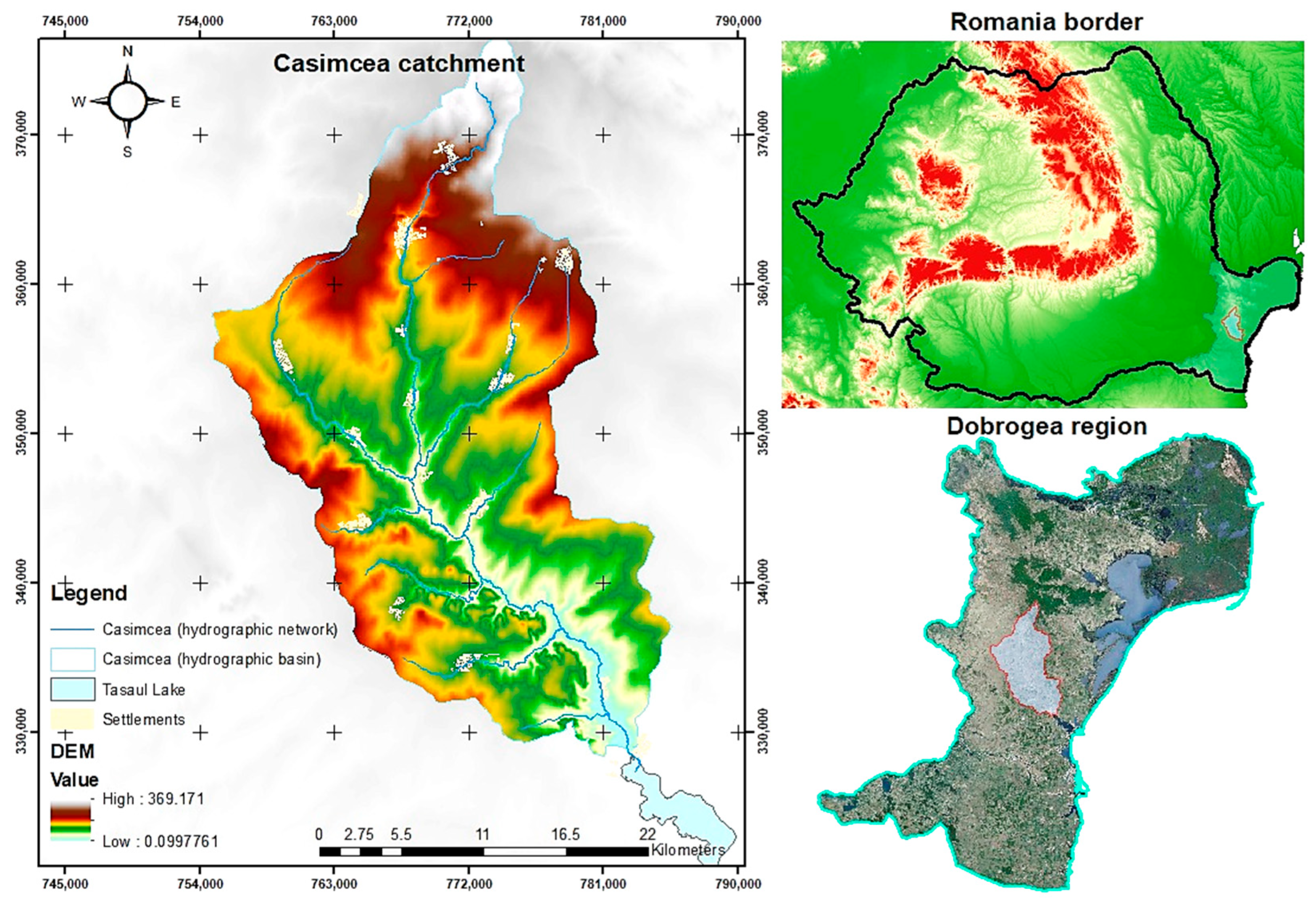
Figure 1. The Casimcea catchment location and the DEM [18].
Hydrology 12 00172 g001
Figure 3. Hydrological network of Casimcea catchment (1-Casimcea, 2-Ramnic, 3-Cartal, 4-Cheia, 5-Casian).
Hydrology 12 00172 g003
Figure 4. Proposed methodology (legend: EDA, Exploratory Data Analysis; EDF, empirical distribution function; PDF, probability distribution function).
Hydrology 12 00172 g004
Figure 5. Variation in maximum discharges for all hydrometric stations.
Hydrology 12 00172 g005
Figure 6. Histogram for the Casimcea station.
Hydrology 12 00172 g006
Figure 7. Histogram for the Cheia station.
Hydrology 12 00172 g007
Figure 8. Histogram for the Cartal station.
Hydrology 12 00172 g008
Figure 9. Histogram for the Râmnic station.
Hydrology 12 00172 g009
Figure 10. Results of the Mann–Kendall test for the Casimcea hydrometric station.
Hydrology 12 00172 g010
Figure 11. FDC for the Casimcea hydrometric station.
Hydrology 12 00172 g011
Figure 12. Probability plots for all stations.
Hydrology 12 00172 g012
Figure 13. Over-ranking relationship for the Râmnic River at the Râmnic station.
Hydrology 12 00172 g013
Figure 14. Confidence interval performance analysis.
Hydrology 12 00172 g014aHydrology 12 00172 g014b
Table 1. Equations for exceedance probability (general formula F x = i α n + 1 2 α , 0 < α 0.5 , where i represents the rank, and n represents the total number of events).
αDefining EquationName (Proponent)
0 F x = i n + 1 Weibull (probability unbiased)
0.3 F x = i 0.3 n + 0.4 Cegodaev (empirical)
0.4 F x = i 0.4 n + 0.2 Cunnane (empirical)
0.5 F x = i 0.5 n Hazen (empirical)
Table 2. Descriptive statistics.
Hydrometric StationLength of Record
Years
Q Mean
(m3/s)
Q max/Data
(m3/s)
Q min
(m3/s)
Standard DeviationSkewnessDrainage Area
(km2)
Average Elevation
(m)
Casimcea5732.43398/20020.04864.544.2778263
Cheia3465.9384/20050.599.702.18500158
Cartal5649.9488/19850.192.863.06128150
Ramnic5623.5131/19880.07629.611.9889166
Table 3. Floods inventory.
NoRiverHydrometric Station/Discharge Equivalent to the Alert Thresholds * in (m3/s)DateThe Maximum Discharge Qmax (m3/s)Precipitation Causing the Qmax
On the Day of the Flood (mm)Precipitation During the 10 Previous Days (mm) *
1CasimceaCasimcea
QaQiQp
1.05.0028.023.10.1964104
13.06.198899.374
03.06.197289.3
30.05.200239894
03–04.07 200558.691 (73 in 3 h)
2CasimceaCheia
QaQiQp
5.072.003.07.20053844427
31.05.20023331027
28.08.20042877725
17.06.2007262
3CartalCartal
QaQiQp
6.916.480.011.06.1985488
24.09.1968316
03.07.200531059 (24 in 30 min)
4RâmnicRamnic
QaQiQp
6.760.922.05.198813125
04.06.1972114
11.06.19941101233
* Qa = warning/attention discharge; Qi = flooding discharge; Qp = danger discharge.
Table 4. Mann–Kendall and Sen’s slope methods.
Time SeriesFirst YearLast YearnTest ZSignific.Sen’s Slope Estimate
Q Casimcea1965202157−2.130.05−0.194
Q Cheia1988202134−2.310.05−0.908
Q Cartal1965202157−2.240.05−0.247
Q Ramnic1965202157−2.110.05−0.232
Table 5. Khronostat software results.
Hydrometric
Station
Period
(Years)
Mean
(m3/s)
Khronostat Results for Independence
Rank CorrelationBuishardPettittLee & HeghinianHubert
ResultsYearResultsYear
Casimcea5726.03rejected at 95% confid.rejected at 90% confid.rejected at 95% confid.1989rejected Ho1989accepted
Cheia3455.0rejected at 95% confid.rejected at 95% confid.rejected at 95% confid.2007rejected Ho2007accepted
Cartal5750.8rejected at 95% confid.rejected at 95% confid.rejected at 95% confid.2006rejected Ho2006accepted
Ramnic5723.9rejected at 90% confid.rejected at 95% confid.rejected at 90% confid.2006rejected Ho2006accepted
Table 6. The maximum discharge values extracted from FDC for different exceedance probabilities.
Maximum Discharge (m3/s)
EDFHazen
Return period (year)
Hydrometric station
10050201052
Casimcea262157.8789.365.450.310.7
Cheiano377.9231012856.212.9
Cartal333324.7228724683.124.3
Ramnic131119.8511057.239.812.6
EDFWeibull
Casimcea262224.3599.373.350.310.7
Cheiano333297.8724683.124.3
Cartal488460.4831622456.212.9
Ramnic131128.12114.0068.839.812.6
Table 7. Results from Hydrognomon for the Casimcea hydrometric station.
Kolmogorov–Smirnov Testa = 1%RankDmax
GammaACCEPT10.0796
Pearson-IIIACCEPT20.0831
GEV-MinACCEPT30.0847
EV3-Min (Weibull, L-moments)ACCEPT40.098
EV3-Min (Weibull)ACCEPT50.1052
Pareto (L-moments)ACCEPT60.1200
GEV-Min (L-moments)ACCEPT70.1215
Table 8. Accepted distribution functions based on rank.
PDFGammaPearson-IIIGEV-MinEV3-Min (Weibull, L-Moments)EV3-Min (Weibull)Pareto (L-Moments)GEV-Min (L-Moments)GEV-Max (L-Moments)Log Pearson-III
Hydrometric Station
Casimcea1234567xx
Cheia7xx631425
Cartal7x6215543
Ramnic2xx56341x
Table 9. Maximum discharge values are predicted using the five chosen PDFs for different return periods. Example for the Casimcea station.
Return Period (T)
Hydrometric Station and PDF’s
100010050201052
Casimcea—Qmax (m3/s)
Gamma323.522193.42155.808107.94373.825342.62489.93832
EV3-Min (Weibull, L-Moments)376.839201.90157.07104.16269.471840.032410.9478
EV3-Min (Weibull)361.019196.20153.516102.76669.178240.368711.3719
Pareto (L-Moments)469.357200.59149.69996.685665.167539.525812.8146
GEV-Min (L-Moments)331.602187.72149.211102.36470.446942.14611.9543
EDF 262157.889.365.450.310.7
Note: GEV—Generalized Extreme Value; EV3—extreme value type 3.
Table 10. Results of the calibration: the observed exceedance probability values were extracted using the Hazen and Weibull equations, respectively.
HazenWeibull
RankrRMSENSER2rRMSENSER2
Casimcea
Gamma10.9629.400.870.920.9839.870.810.92
EV3-Min (Weibull, L-Moments)20.9725.680.900.950.9837.150.840.95
EV3-Min (Weibull)30.9727.820.890.940.9839.740.810.94
Pareto (L-Moments)40.9825.860.900.970.9939.870.810.97
GEV-Min (L-Moments)50.9731.240.860.940.9843.300.780.94
Cheia
Pareto (L-Moments)10.8773.340.620.760.9356.670.740.87
EV3-Min (Weibull)20.9080.060.550.800.9456.910.740.88
GEV-Min (L-Moments)30.9252.440.810.850.9353.700.770.86
EV3-Min (Weibull, L-Moments)40.9060.020.750.810.82172.03−1.400.67
Gamma50.9060.020.750.810.9453.910.760.88
Cartal
EV3-Min (Weibull)10.9849.000.920.800.9779.970.810.93
EV3-Min (Weibull, L-Moments)20.9838.520.750.810.9867.810.860.92
Pareto (L-Moments)30.9658.720.620.760.9692.350.740.86
GEV-Min (L-Moments)40.9745.350.810.850.9772.520.840.91
Gamma50.9940.540.750.810.9968.580.860.96
Râmnic
Gamma10.8637.360.290.740.8338.430.280.70
Pareto (L-Moments)20.7968.69−1.410.620.7569.22−1.330.57
GEV-Min (L-Moments)30.8734.920.380.760.8246.06−0.030.67
EV3-Min (Weibull, L-Moments)40.8261.21−0.910.680.7944.37−0.840.63
EV3-Min (Weibull)50.8443.350.040.710.8161.550.040.66
Table 11. Criteria and values for performance parameters.
PerformancerRMSE/STDEVNSER2
very good0.80–10.0–0.50.80–10.80–1
good0.6–0.80.5–0.60.70–0.800.6–0.8
satisfactory0.4–0.60.6–0.70.5–0.700.4–0.6
unsatisfactory<0.4>0.7<0.5<0.4
Table 12. The criteria and weight.
CriteriaAchieved arRRSNSER2
weight0.500.120.130.130.12
Table 13. Results of the ELECTRE method.
Model (M)Net Superior ValueRankNet Superior ValueRankObservation
Casimcea
M1 (Gamma)0.3903−2.8622E
M2 (EV3-Min-Weibull, L-Moments)2.6501−3.0571
M3 (EV3-Min Weibull)0.00040.0363E
M4 (Pareto-L-Moments)0.48021.8834E
M5 (GEV-Min-L-Moments)−3.52054.0005
Cheia
M1 (Pareto-L-Moments)0.1302−0.7292
M2 (EV3-Min-Weibull)−0.13030.0503
M3 (GEV-Min-L-Moments)2.0001−1.2961
M4 (EV3-Min Weibull, L-Moments)−0.50041.0005E
M5 (Gamma)−1.50050.9754E
Cartal
M1 (EV3-Min-Weibull)1.5102−2.9562
M2 (EV3-Min-Weibull, L-Moments)2.2601−2.9761
M3 (Pareto-L-Moments)−2.00050.7313E
M4 (GEV-Min-L-Moments)−0.50031.6144E
M5 (Gamma)−1.27043.5885E
Ramnic
M1 (Gamma)1.1302−2.3201
M2 (Pareto-L-Moments)0.13031.9664
M3 (GEV-Min-L-Moments)2.0001−2.2672
M4 (EV3-Min-Weibull, L-Moments)−1.26040.2823
M5 (EV3-Min-Weibull)−2.00052.3395
Table 14. Aggregate dominance matrix.
CartalM1M2M3M4M5
M101011
M210000
M300011
M400000
M500000
Disclaimer/Publisher’s Note: The statements, opinions and data contained in all publications are solely those of the individual author(s) and contributor(s) and not of MDPI and/or the editor(s). MDPI and/or the editor(s) disclaim responsibility for any injury to people or property resulting from any ideas, methods, instructions or products referred to in the content.