Just a Single-Layer CNN for Stochastic Modeling: A Discriminator-Free Approach

Abstract

The advent of machine learning (ML) has significantly transformed hydrology, particularly in the simulation of hydrological flows. However, ML techniques have not been employed to the same extent in stochastic hydrology. In applied sciences, the most common ML-based approach for developing stochastic simulation schemes is the use of generative adversarial networks (GANs), which consist of two sub-models, that is, a generator and a discriminator. Despite their potential, GANs have notable limitations, including high architectural complexity and the requirement to divide observed time series into shorter segments to generate sufficient training examples. This segmentation reduces the effective length of the series, limiting the model’s ability to capture and reproduce long-term dependencies. In this study, we propose a simpler stochastic scheme based on a single convolutional neural network (CNN) used as a generator, replacing the discriminator component of the GAN with a specifically designed cost function. The model is applied to a case study involving measured flow velocity time series and evaluated against traditional stochastic schemes designed for both Markovian and Hurst–Kolmogorov processes. Results show that the CNN-based approach not only offers computational simplicity but also outperforms conventional methods in preserving key statistical characteristics of the observed data.

1. Introduction

In recent years, machine learning (ML) has achieved remarkable milestones across a range of disciplines, often demonstrating capabilities that surpass human performance. Notable examples include AlphaGo, which defeated world champions in the complex game of Go; AlphaFold, which revolutionized protein structure prediction; and ResNet, which significantly advanced the field of computer vision [1]. Despite these groundbreaking achievements, the mathematical foundations of such models remain relatively simple. For instance, large language models (LLMs), like GPT-4, exhibit advanced reasoning and nuanced language understanding, yet they operate through a simple probabilistic token sampling process based on the distribution $P\left(w_t\right|w_1,w_2,...,w_{t-1})$, where $w_t$ is the token at position t in the sequence [2]. At their core, machine learning models are fundamentally statistical in nature.

Beginning almost three decades ago, ML techniques have gained significant traction in hydrology due to their ability to model complex, nonlinear processes without requiring explicit physical formulations. For instance, artificial neural networks (ANNs) have long been employed for runoff discharge prediction (e.g., Ref. [3]). More recently, long short-term memory (LSTM) networks, a form of recurrent neural networks, have demonstrated excellent performance in capturing temporal dependencies in streamflow time series (e.g., Ref. [4]). In groundwater hydrology, support vector regression (SVR) has been applied for modeling groundwater levels [5], while random forest (RF) algorithms have shown promise in regional hydrological frequency analysis [6]. Additionally, convolutional neural networks (CNNs) have been used to estimate discharge in ungauged watersheds, utilizing satellite imagery as input features [7]. These examples highlight the growing role of ML in addressing the limitations of traditional, physically based hydrological models. However, one subfield where ML applications remain limited is stochastic hydrology.

Stochastic approaches play a pivotal role in applied sciences such as hydrology and economics, where uncertainty, variability, and incomplete information are inherent features of the systems studied. Both natural and anthropogenic processes exhibit intrinsic randomness that deterministic models alone cannot fully capture. In hydrology, stochastic models are essential for simulating rainfall, streamflow, and groundwater fluctuations—in the sense of generating equiprobable alternative realizations—enabling more realistic assessments of risk and variability under changing climate conditions [8]. Likewise, in economics, stochastic modeling forms the backbone of financial forecasting, market dynamics, and decision-making under uncertainty [9]. A fundamental element in both fields involves the analysis of time series, which provides valuable insight into temporal patterns, trends, cycles, and memory effects, including long-range dependence. Understanding and modeling these temporal structures is essential for developing robust predictions and management strategies.

Among machine learning algorithms, generative adversarial networks (GANs) are particularly well-suited to stochastic analysis due to their design for generative modeling. The generator aims to produce synthetic data that mimics real observations, while the discriminator learns to distinguish between real and synthetic data. Through this adversarial process, the generator progressively improves its ability to capture the underlying stochastic structure of the training distribution [10].

GANs are especially valuable in stochastic modeling because they do not rely on predefined assumptions about the form of the probability distribution. Instead, they learn complex, high-dimensional distributions directly from data [10]. This makes them well-suited for generating equiprobable synthetic time series, spatial fields, or future scenarios. Although initially applied mainly to image generation, the potential of GANs for hydrological applications was quickly recognized [11], whereas in the field of economics, a particularly influential study by Takahashi et al. [12] demonstrated that GANs could replicate the statistical properties of historical financial time series. Takahashi et al. assessed GANs’ ability to reproduce specific “stylized facts” of financial time series, including properties of temporal correlation (such as linear unpredictability and volatility clustering) and distributional characteristics (such as fat tails). GANs showed impressive performance in capturing and reproducing these features. Subsequently, GANs have been applied to hydrology for similar tasks, including weather generation [13], synthetic runoff series for multi-reservoir management [14], and stochastic simulation of delta formation [15].

GANs are particularly effective in time series applications because of their capacity to learn and replicate abstract features of stochastic processes, provided the generator and discriminator are properly balanced and trained on a sufficient number of examples [16,17]. In time series modeling, this typically involves segmenting historical records into multiple shorter samples. However, this segmentation can undermine the inference of long-term statistics, which are crucial in many hydrological and economic contexts. To address this limitation, Shaham et al. [18] proposed SinGAN, a scheme that can be trained on a single example. SinGAN employs a pyramid of GANs, where lower layers operate on small subregions of the training example, and higher layers progressively cover larger areas. This hierarchical structure allows the model to extract fine-scale statistics from localized subregions and coarse-scale statistics from the entire dataset.

Figure 1 presents a schematic of a typical GAN, illustrating its two key components, that is, the generator and the discriminator. Although the architecture is simpler than that used in other advanced ML applications, such as LLMs, it still entails a certain level of complexity. A standard GAN generator typically includes four transposed convolutional layers, while the discriminator consists of a similar number of convolutional layers [19]. When employing SinGAN, which is essential for preserving long-term statistics as previously discussed, the architectural complexity increases proportionally with the number of GAN layers used.

The complexity of GANs introduces certain requirements regarding the computational resources needed for network training, both in terms of capacity and time. Moreover, in applied hydrology, practitioners often face challenges in adopting sophisticated tools due to limited technical familiarity. To address this issue, Rozos et al. [20] proposed a simplified approach based on a multilayer perceptron (MLP) with fourteen input nodes, two hidden layers (each with two nodes), and a single output node. The simplicity of the network takes advantage of the annual periodicity encoded in the input data, while the cost function computes the deviation between the statistical characteristics of the synthetic and observed time series. It evaluates key properties across multiple scales (daily, annual, and higher), as well as wet/dry state frequencies and transition probabilities. Since the cost function lacks an analytical expression for its derivative with respect to the network’s output, a genetic algorithm was used for training, resulting in relatively long training times. Once trained, the MLP can be implemented in a standard spreadsheet environment. This approach is suitable for simulating a single intermittent stochastic process with periodicity, such as daily rainfall.

This study focuses on the stochastic modeling of multivariate continuous and regular (non-intermittent, non-periodic) processes. Such processes are prevalent in hydrological applications, where the generative adversarial network (GAN) framework represents a recent and significant advancement in stochastic modeling due to its ability to capture complex data distributions. Consider soil moisture, a crucial hydrological variable that regulates vegetation growth and environmental health. GANs have been successfully employed for generating spatiotemporal time series of soil moisture indices in the context of drought forecasting [21]. Similarly, the flow discharge of non-ephemeral rivers exemplifies another hydrological process within this category. For instance, a GAN incorporating mass conservation constraints has been utilized for forecasting extreme flood events [22], thereby supporting early warning systems. Furthermore, a variation of this approach has been applied to flood risk mapping for identifying vulnerable regions [23]. From a broader perspective, continuous and regular processes are ubiquitous in geophysical sciences. Characteristic examples related to natural hazards include seismic waves generated by earthquakes, sea surface temperature (linked to localized atmospheric hazards like hurricanes), and groundwater levels (a key controlling factor in landslide occurrences). Generative deep learning has demonstrated high efficiency and broad applicability across these diverse domains [24].

In this study, a novel ML-based approach suitable for multivariate non-intermittent, non-periodic processes is proposed. The conceptual design draws inspiration from the GAN framework but omits the discriminator component to both simplify the architecture and avoid the dilemma of either segmenting the data or employing more complex models like SinGAN. In the proposed model, a single convolutional layer replaces the GAN generator, operating on white noise inputs to produce synthetic data. Unlike the work of Rozos et al. [20], the cost function is designed to have analytical derivatives, allowing for efficient training via backpropagation. The simplicity of the architecture—centered on a single convolutional layer—makes it feasible to implement the trained model in practitioner-friendly platforms such as spreadsheets.

The proposed method was tested using flow velocity measurements from the Laboratory of Hydromechanics at the University of Siegen [25]. The magnitudes of the velocity vectors along the three spatial axes (x, y, z) were treated as a trivariate stochastic process. For benchmarking purposes, conventional stochastic models—a Markovian model and a Hurst–Kolmogorov model—were also applied to the same dataset.

2. Materials and Methods

2.1. Measurements

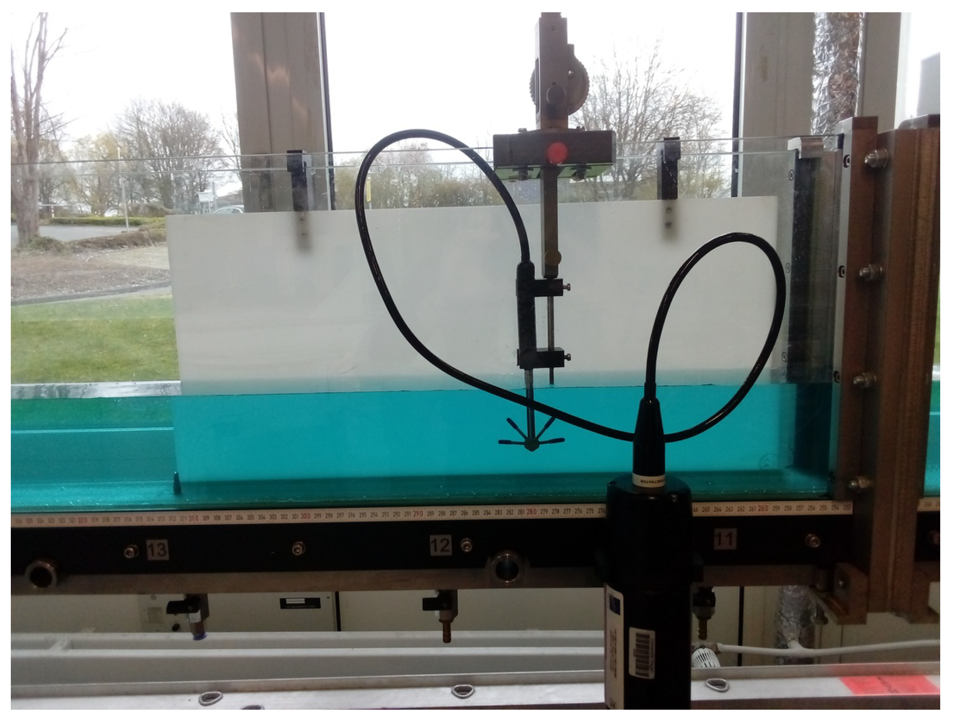
The dataset was obtained from flow measurements conducted in a hydraulic channel with a width of 8.5 cm and a length of 5 m. The flow depth during the experiment was maintained at 15.2 cm, and the discharge was set to 3.2 L/s. Flow velocity measurements were acquired using an acoustic Doppler velocimeter (ADV) equipped with a side-looking probe. The experimental setup is illustrated in Figure 2. Further details are provided in Ref. [25].

2.2. Second-Order Characteristics of Stochastic Process—The Climacogram

As previously mentioned, evaluating the deviation of statistical characteristics between synthetic and observed time series is central to the proposed machine learning scheme. These characteristics are described using statistical moments, which, for stationary stochastic processes, remain invariant over time. The most commonly used metrics are the mean, variance, and skewness, which correspond to the first three moments of the first-order distribution function. Higher-order classical moments, however, are considered unknowable in practice due to limitations in their estimation, as discussed in [26].

Solely preserving these first-order metrics is insufficient for most real-world processes. In such cases, second-order characteristics, such as the autocovariance function, must also be accurately represented. However, the use of the autocovariance function has recently been criticized due to its mathematical formulation—it is the second derivative of the climacogram, normalized by the variance—which can lead to misinterpretations of a process’s behavior [27].

Alternative second-order statistical metrics include the variogram, the power spectrum, and the climacogram, all of which are mathematically equivalent transformations. Despite this equivalence, they differ significantly in terms of practical application. Among these, the climacogram is gaining popularity due to its lower statistical bias and reduced uncertainty, especially when working with small datasets [27].

The climacogram, introduced by Koutsoyiannis [28], is conceptually straightforward. It shows how the variance of a dataset evolves as the data are aggregated over increasing time scales (e.g., using moving averages). By plotting the variance against the time scale on a log–log graph, the climacogram reveals the underlying statistical structure of the process. One of its key insights is persistence, which is quantified by the Hurst parameter H. The parameter H ranges from 0 to 1, with values greater than 0.5 indicating a persistent process. The slope of the climacogram at larger scales is equal to $2H-2$.

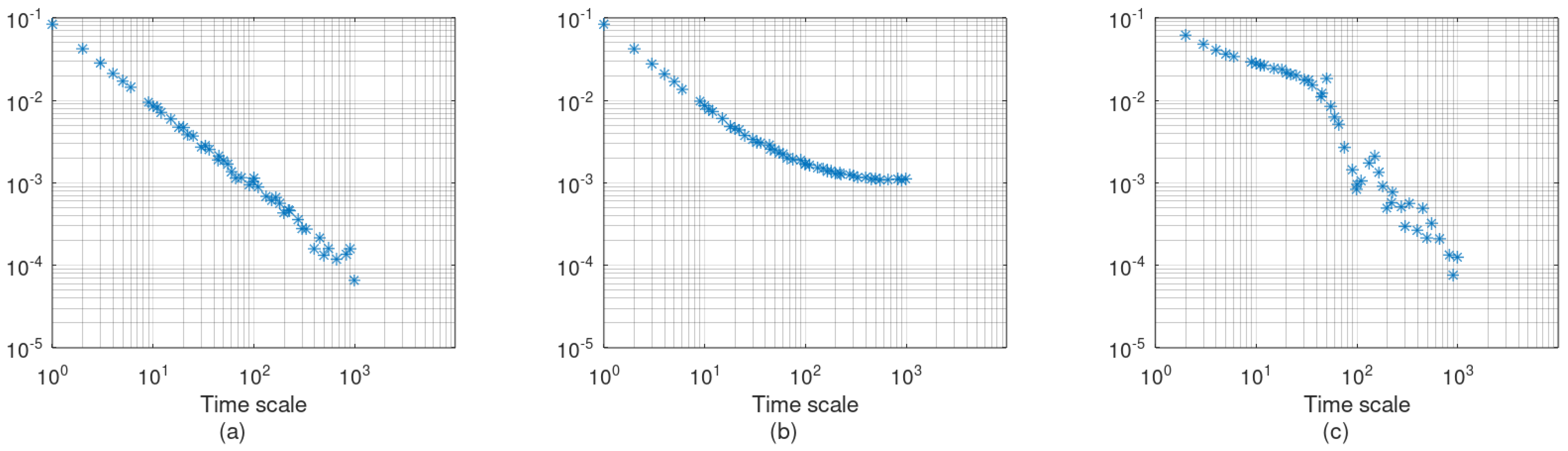
Figure 3 illustrates three examples of climacograms:

• Figure 3a shows the climacogram of a random signal, exhibiting the typical slope of $-1$ and a Hurst parameter of 0.5. This slope is also characteristic of all Markovian processes, although their climacograms tend to flatten at small scales.
• Figure 3b presents a random signal combined with a linear trend. At small scales, the slope is $-1$, as in a pure random signal, but it increases (tends toward zero) at larger scales as the deterministic trend dominates.
• Figure 3c shows a random process combined with a sinusoidal signal with a period of 100 time units. Initially, the climacogram has a mild negative slope, which steepens as the time scale approaches the period of the sinusoidal signal, where variance drops sharply. Beyond that, the slope gradually returns to $-1$, with some oscillations due to the harmonics.

These examples demonstrate the diagnostic power of the climacogram in analyzing the structure of stochastic processes. For this reason, it is adopted here as the primary metric for assessing model performance with respect to second-order statistics. First-order characteristics will be evaluated using conventional metrics such as mean, variance, skewness, covariance, and histograms.

2.3. Markovian Model (AR1)

The first-order autoregressive scheme (AR1) is among the most widely used stochastic models for capturing the essential structure of temporal dependence in time-series data. Its simplicity and analytical tractability make it particularly attractive for modeling processes that exhibit short-term memory. 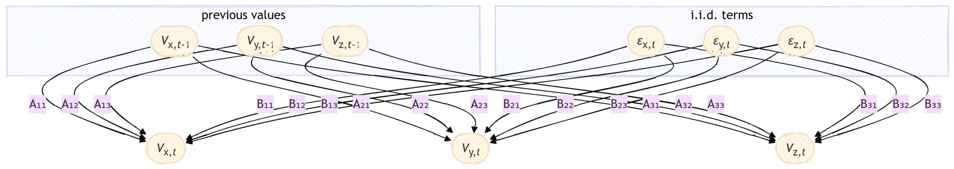In hydrology, multivariate extensions of AR1 have been employed to simulate and forecast multiple interrelated hydrological variables, with varying degrees of success, depending on system complexity and data quality [29]. The multivariate AR1 can be expressed as follows:

$${\mathit{V}}_t=\mathit{A}{\mathit{V}}_{t-1}+\mathit{B}{\mathit{ϵ}}_t,$$

(1)

where t denotes the time index. In the case of the three variables, ${\mathit{V}}_t$ is a 3 × 1 vector containing the values of the variables at time step t, and ${\mathit{ϵ}}_t$ is a 3 × 1 vector of independent and identically distributed (i.i.d.) random variables. The matrix $\mathit{A}$ is the 3 × 3 coefficient matrix representing the linear dependence between time steps, and $\mathit{B}$ is the 3 × 3 innovation matrix that scales the noise components.

Note: For simplicity, all matrix dimensions hereinafter are presented assuming the specific case of the three variables used in this study. However, generalization to an arbitrary number of variables is straightforward.

The matrices $\mathit{A}$ and $\mathit{B}$ can be estimated directly from the observational data using the following formulas:

$$\mathit{A}=\mathbf{cov}(\mathit{V},{\mathit{V}}_1)\mathbf{cov}{\left(\mathit{V}\right)}^{-1},$$

(2)

$${\mathit{B}\mathit{B}}^{\mathrm{T}}=\mathbf{cov}\left(\mathit{V}\right)-\mathit{A}\mathbf{cov}\left(\mathit{V}\right){\mathit{A}}^{\mathrm{T}},$$

(3)

where $\mathbf{cov}(·,·)$ denotes the sample cross-covariance matrix between its arguments, and $\mathbf{cov}(·)$ denotes the sample covariance matrix. The matrix $\mathit{V}$ is constructed such that each column t contains the values of the three variables at time step t, while ${\mathit{V}}_1$ is obtained by a horizontal circular shift of $\mathit{V}$, meaning that column t of $\mathit{V}$ corresponds to column $t+1$ of ${\mathit{V}}_1$.

Note that in this case study, the matrix $\mathit{V}$ has three rows, corresponding to each component of the flow velocity vector in the x-, y-, and z-directions. The covariance matrix $\mathbf{cov}\left(\mathit{V}\right)$ is, therefore, a 3 × 3 matrix, with the covariances between ${\mathit{V}}_{\mathrm{x}}$, ${\mathit{V}}_{\mathrm{y}}$, and ${\mathit{V}}_{\mathrm{z}}$ as off-diagonal elements, and the corresponding variances on the diagonal.

The right-hand sides of Equations (2) and (3) can be directly computed from the observed data. If the resulting matrix on the right-hand side of Equation (3) is positive definite, the innovation matrix $\mathit{B}$ can be estimated by a straightforward matrix decomposition of $\mathit{B}\mathit{B}$. In this study, eigendecomposition was used for this purpose [30]. In cases where the matrix is not positive definite, more advanced decomposition techniques are required [31].

To ensure that the skewness of the original process is preserved, the statistical estimator ${\mathsf{\mu }}_3\left(\mathit{ϵ}\right)$—a 3 × 1 vector representing the third central moments of the i.i.d. terms—should satisfy the following relation [30]:

$${\mathsf{\mu }}_3\left(\mathit{ϵ}\right)={\mathit{B}}^{\circ (-3)}({\mathsf{\mu }}_3\left(\mathit{V}\right)-{\mathsf{\mu }}_3\left(\mathit{A}\mathit{V}\right)),$$

(4)

Note that the “∘” (Hadamard notation) explicitly states that the exponentiation is element-wise.

For the generation of $\mathit{ϵ}$, a random number generator based on the Generalized Pareto distribution was used to produce three time series (one for each row of $\mathit{ϵ}$) with zero mean, unit standard deviation, and a third central moment equal to ${\mathsf{\mu }}_3\left(\mathit{ϵ}\right)$.

A schematic representation of the AR1 algorithm is shown in Figure 4.

AR1 is most appropriate for modeling Markovian processes, where the future state depends only on the present state (although other unknown influences may exist). A characteristic feature of such processes is that their autocovariance function decays exponentially with increasing lag.

2.4. Hurst–Kolmogorov Model (HK)

Physical processes that exhibit substantial persistence—manifested as prolonged periods of similar values—are more accurately described by Hurst–Kolmogorov (HK) stochastic processes. These processes differ from Markovian ones in that they feature long-range dependence, which significantly affects their statistical behavior and modeling approach. For a single process, such as $\underline{V_{\mathrm{x}}}$, a moving average (MA) scheme can be employed to generate synthetic time series:

$$V_{\mathrm{x}t}=\sum _{j=-J}^J{a}_j{\mathit{ϵ}}_{t-j}$$

(5)

where $a_j$ are coefficients calculated by the following formula [27]:

$$a_j=\sqrt{{\displaystyle \frac{2(1-H)}{{(1.5-H)}^2}}\mathrm{var}\left({\mathit{V}}_{\mathrm{x}}\right)}\left({0.5|j+1|}^{H+0.5}{+0.5|j-1|}^{H+0.5}-{\left|j\right|}^{H+0.5}\right)$$

(6)

The previous moving average scheme is a univariate stochastic model. For multivariate processes, Equation (5) needs to be applied to each component individually, using modified i.i.d. terms ${\mathit{ϵ}}^{\prime }$ that incorporate the covariance structure of the multivariate system. These terms are derived from the following transformation [32]:

$${{\mathit{ϵ}}^{\prime }}_t=\mathit{b}{\mathit{ϵ}}_t$$

(7)

where the 3 × 3 matrix $\mathit{b}$ is given by the following formula:

$$\mathit{b}{\mathit{b}}^{\mathrm{T}}=\mathit{c}$$

(8)

where $\mathit{c}$ is a 3 × 3 matrix whose elements are derived from the normalized covariance values of the original variables. Specifically, each element of $\mathit{c}$ corresponds to the covariance between a pair of variables, divided by the sum of the products of their respective MA weights $a_j$. For instance, if $c_{21}$ represents the covariance between ${\mathit{V}}_{\mathrm{x}}$ and ${\mathit{V}}_{\mathrm{y}}$, it is calculated using the following formula [32]:

$$c_{21}=\mathrm{cov}({\mathit{V}}_{\mathrm{x}},{\mathit{V}}_{\mathrm{y}})/\sum _{j=-J}^J{a}_{\mathrm{x}j}{a}_{\mathrm{y}j}$$

(9)

Then, the matrix $\mathit{b}$ is computed from $\mathit{b}{\mathit{b}}^{\mathrm{T}}$ using the eigendecomposition method.

If the skewness of the process is significant, then this characteristic should be preserved by the stochastic scheme. For the trivariate case study, the skewnesses of the three-row matrix ${\mathit{ϵ}}^{\prime }$ are represented by the vector ${\mathit{\xi }}_{{\mathit{ϵ}}^{\prime }}$. The first element of this vector, corresponding to the x-direction, is related to the estimated skewness of $\underline{V_{\mathrm{x}}}$ according to the following formula (the formulas for the other two dimensions are similar):

$${\xi }_{{{\mathit{ϵ}}^{\prime }}_{\mathrm{x}}}={\xi }_{V_{\mathrm{x}}}\mathrm{var}{\left({\mathit{V}}_{\mathrm{x}}\right)}^{3/2}\sum _{j=-J}^J{a}_{\mathrm{x}j}^3$$

(10)

The skewness of $\mathit{ϵ}$ can be calculated from the skewness of ${\mathit{ϵ}}^{\prime }$ with the following formula [32]:

$${\mathit{\xi }}_{\mathit{ϵ}}={\mathit{\xi }}_{{\mathit{ϵ}}^{\prime }}{\mathit{b}}^{\circ (-3)}$$

(11)

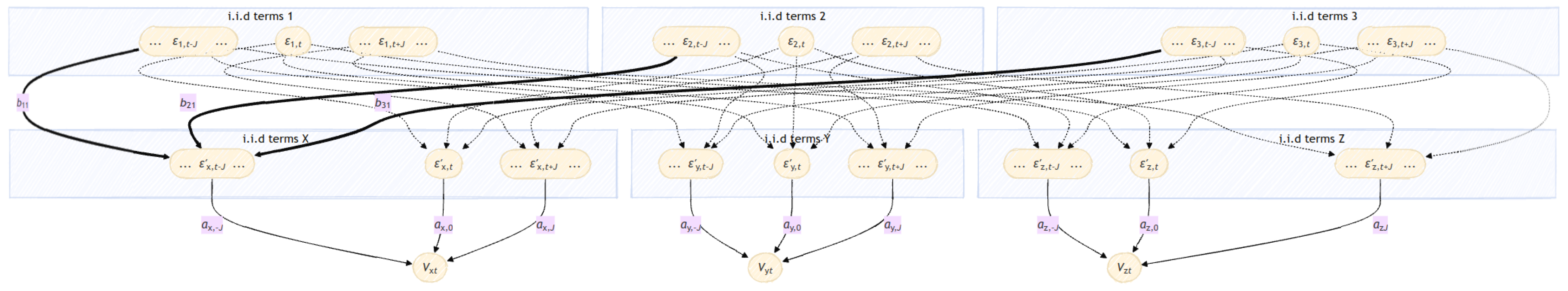
The schematic representation of the algorithm is displayed in the following figure. Three time series of i.i.d. terms are produced with a random number generator that follows the Generalized Pareto distribution with a mean equal to zero, a standard deviation equal to 1, and skewness ${\mathit{\xi }}_{\mathit{ϵ}}$. These random numbers are organized into the three-row matrix $\mathit{ϵ}$. Then, by applying Equation (7), these time series are transformed into time series of i.i.d. terms, organized into the three-row matrix ${\mathit{ϵ}}^{\prime }$. The time series of ${\mathit{ϵ}}^{\prime }$ have zero self-correlation in time, but are correlated with each other. The moving average scheme of Equation (5) is applied independently to each of the time series of ${\mathit{ϵ}}^{\prime }$ to produce synthetic values of the simulated variables.

A schematic representation of the algorithm of the HK scheme is displayed in Figure 5.

This scheme can preserve the autocovariance function up to a lag equal to J (see Figure 3 in Ref. [32]).

2.5. Autoregressive Integrated Moving Average

The combination of autoregressive (AR) and moving average (MA) schemes yields the versatile autoregressive moving average (ARMA) stochastic model. The autoregressive integrated moving average (ARIMA) model extends ARMA by incorporating a differencing operator, enabling it to accommodate non-stationary data characterized by trends or varying means. Further generalizing ARIMA, autoregressive fractional integrated moving average (ARFIMA) models introduce fractional differencing (non-integer orders of integration). This feature provides a natural framework for modeling long-memory processes, in which the autocorrelation function exhibits a slow, hyperbolic decay.

ARFIMA models are defined by the triplet of parameters $(p,d,q)$, where p and q denote the orders of the AR and MA components, respectively, and d represents the degree of differencing. The value of d is contingent upon the nature of the stochastic process being modeled. Specifically, if $d\in [-0.5,0.5]$, the ARFIMA model can effectively simulate a stationary process [33].

In the present study, the ARFIMA model, implemented in MATLAB R2021b, was employed. This implementation was developed by building upon the contributions of Fatichi, Caballero, and Inzelt. A comparative analysis by Liu et al. [34] evaluated this MATLAB-based tool against an ARFIMA implementation in R, demonstrating virtually identical simulation results across all test case studies. Given its univariate nature, this specific ARFIMA model cannot be comprehensively compared with the other models examined in this study. Instead, it serves as an initial exploration to estimate the maximum efficiencies attainable with conventional time series models. For this investigation, the orders p and q were set to 2, while the degree of differencing d was estimated by the model itself.

2.6. Machine Learning (CNN)

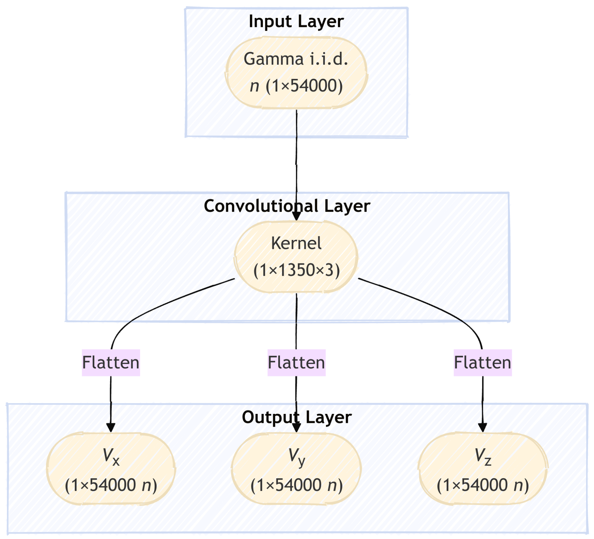
The topology of the CNN model is shown in Figure 6. Typically, the input of a CNN is a structured data grid, most often images represented as multi-dimensional arrays (e.g., RGB images as height × width × 3 tensors). In this study, each input instance is a one-dimensional array of size 1 × 54,000, where each of the 54,000 values is drawn from a Generalized Pareto distribution. The instance size matches the length of the observed time series (54,000 values). Consequently, the total length of synthetic values generated by the CNN is 54,000n, where n is the number of instances. The hidden layer is a convolutional layer with a kernel of 3 channels (dimensions: 1 × 1350 × 3). Each channel produces the synthetic values for one of the three stochastic variables simulated (i.e., the three components of flow velocity along the primary axis). No activation function is applied.

The input features (i.i.d. values) have a mean of 0 and a standard deviation of 1. This does not affect the CNN’s ability to reproduce the mean and standard deviation of the observed time series; the mean of the output is primarily influenced by the bias terms, while the standard deviation is determined by the scale of the kernel weights. In contrast, skewness is more implicitly influenced by the CNN weights, as inferred from Equation (10).

To ensure the skewness of the output matches that of the observed time series, the skewness of the features imposes a constraint on the kernel weights via Equation (10). In practice, setting the feature skewness to 4–5 times the largest observed absolute skewness minimizes the restrictive influence of this constraint.

The training methodology follows the approach used by Rozos et al. [20]. The cost function compares outputs to observed data not by direct distance, but by differences in statistical metrics. It is defined as follows:

$$C\left(\mathit{y}\right)=\left[W_1\dots W_5\right]·\left[\begin{array}{c}\mathrm{D}\left({({\mathit{C}}_{\mathrm{S}}-{\mathit{C}}_{\mathrm{O}})}^{\circ 2}\right)\\ \mathrm{D}\left({({\mathit{C}}_{1\mathrm{S}}-{\mathit{C}}_{1\mathrm{O}})}^{\circ 2}\right)\\ \mathrm{D}\left({({\mathit{\gamma }}_{T\mathrm{S}}-{\mathit{\gamma }}_{T\mathrm{O}})}^{\circ 2}\right)\\ \mathrm{D}\left({({\mathit{\xi }}_{\mathrm{S}}-{\mathit{\xi }}_{\mathrm{O}})}^{\circ 2}\right)\\ \mathrm{D}\left({({\mathit{\mu }}_{\mathrm{S}}-{\mathit{\mu }}_{\mathrm{H}})}^{\circ 2}\right)\end{array}\right]$$

(12)

where $\mathit{y}$ is the CNN output; $W_1$ to $W_5$ are cost function weights; ${\mathit{C}}_{\mathrm{S}}$ and ${\mathit{C}}_{\mathrm{O}}$ (3 × 3 matrices) are the covariance matrices of the simulated and observed time series; ${\mathit{C}}_{1\mathrm{S}}$ and ${\mathit{C}}_{1\mathrm{O}}$ are the corresponding lag-1 cross-covariance matrices; ${\mathit{\gamma }}_{T\mathrm{S}}$ and ${\mathit{\gamma }}_{T\mathrm{O}}$ (3 × 1 vectors) are the variances at scale T; ${\mathit{\xi }}_{\mathrm{S}}$ and ${\mathit{\xi }}_{\mathrm{O}}$ are the skewness vectors; and ${\mathit{\mu }}_{\mathrm{S}}$ and ${\mathit{\mu }}_{\mathrm{O}}$ are the mean value vectors. The function D returns the average of all elements in its argument (whether a vector or matrix).

In Rozos et al. [20], the derivative of the cost function with respect to the network output was unavailable analytically, which prevented the use of backpropagation. As a result, an evolutionary algorithm (a genetic algorithm) was employed, although with slow convergence. In this study, the cost function is differentiable (see Appendix A), allowing for efficient training via the backpropagation method [35].

The weights $W_1$ to $W_5$ serve dual purposes, that is, they balance the relative importance of each statistical metric in the cost function and also modulate the learning rate. To prevent exploding gradients, gradient values are rescaled when they exceed a predefined threshold [36]. The training uses the ADADELTA optimization algorithm [37], which dynamically adjusts the learning rate over time and is robust to noisy data.

Each instance is treated as a separate batch during training. No dropout is used, enabling the network to directly learn from the data without introducing stochastic regularization that could hinder the model’s ability to capture dependencies.

As noted earlier, the number of instances, n, defines the length of the synthetic time series. This number can be kept low during training to reduce computational demand and then increased afterward for generation. In this study, n was set to 20 during training and raised to 100 for application.

The CNN scheme was implemented using the Cortexsys framework [38], which is compatible with both MATLAB^® and GNU Octave.

3. Results

This section presents a comparative analysis of the synthetic time series generated by the stochastic schemes—AR1, HK, ARFIMA, and CNN—against the observed data. For the CNN scheme, the results are based on synthetic values produced using a new set of input features (i.e., independently and identically distributed values), distinct from those used during training. This ensures that the evaluation reflects the model’s generalization ability rather than overfitting.

The covariance matrices of the observed and synthetic time series generated by the stochastic schemes AR1, HK, and CNN are shown in

Table 1. Covariance matrix of the observed and synthetic time series.

	Obs.			AR1			HK			CNN
	${\mathit{V}}_{\mathrm{x}}$	${\mathit{V}}_{\mathrm{y}}$	${\mathit{V}}_{\mathrm{z}}$	${\mathit{V}}_{\mathrm{x}}$	${\mathit{V}}_{\mathrm{y}}$	${\mathit{V}}_{\mathrm{z}}$	${\mathit{V}}_{\mathrm{x}}$	${\mathit{V}}_{\mathrm{y}}$	${\mathit{V}}_{\mathrm{z}}$	${\mathit{V}}_{\mathrm{x}}$	${\mathit{V}}_{\mathrm{y}}$	${\mathit{V}}_{\mathrm{z}}$
${\mathit{V}}_{\mathrm{x}}$	1.625	−0.205	−0.023	1.626	−0.206	−0.023	1.619	−0.204	−0.021	1.572	−0.202	−0.025
${\mathit{V}}_{\mathrm{y}}$	−0.205	0.395	0.130	−0.206	0.395	0.138	−0.204	0.395	0.138	−0.202	0.392	0.135
${\mathit{V}}_{\mathrm{z}}$	−0.023	0.130	1.418	−0.023	0.138	1.417	−0.021	0.138	1.420	−0.025	0.135	1.408

. These matrices are symmetric and positive definite, with their diagonals representing the variances of each variable. The covariances of the synthetic time series produced by all three schemes were very close to the observed values.

The lag-1 cross-covariance matrices are presented in

Table 2. Lag-1 cross-covariance matrix of the observed and synthetic time series.

	Obs.			AR1			HK			CNN
	${\mathit{V}}_{\mathrm{x}}$	${\mathit{V}}_{\mathrm{y}}$	${\mathit{V}}_{\mathrm{z}}$	${\mathit{V}}_{\mathrm{x}}$	${\mathit{V}}_{\mathrm{y}}$	${\mathit{V}}_{\mathrm{z}}$	${\mathit{V}}_{\mathrm{x}}$	${\mathit{V}}_{\mathrm{y}}$	${\mathit{V}}_{\mathrm{z}}$	${\mathit{V}}_{\mathrm{x}}$	${\mathit{V}}_{\mathrm{y}}$	${\mathit{V}}_{\mathrm{z}}$
${\mathit{V}}_{\mathrm{x}}$	0.745	0.007	−0.089	0.746	0.005	−0.089	0.201	−0.041	−0.005	0.717	0.006	−0.091
${\mathit{V}}_{\mathrm{y}}$	−0.185	0.094	0.035	−0.186	0.094	0.036	−0.041	0.110	0.040	−0.182	0.093	0.034
${\mathit{V}}_{\mathrm{z}}$	0.009	0.158	0.393	0.009	0.159	0.392	−0.005	0.039	0.429	0.009	0.156	0.385

. These matrices are positive definite but not necessarily symmetric; the elements on their diagonals represent the lag-1 autocovariances of each variable. The matrix generated by the HK scheme was symmetric and deviated from the observed, indicating limitations in capturing directionality in lagged dependencies. In contrast, the matrices from the AR1 and CNN schemes closely matched the observed matrix.

Table 3. Skewness of the observed and synthetic time series.

Obs.			AR1			HK			CNN
${\mathit{V}}_{\mathrm{x}}$	${\mathit{V}}_{\mathrm{y}}$	${\mathit{V}}_{\mathrm{z}}$	${\mathit{V}}_{\mathrm{x}}$	${\mathit{V}}_{\mathrm{y}}$	${\mathit{V}}_{\mathrm{z}}$	${\mathit{V}}_{\mathrm{x}}$	${\mathit{V}}_{\mathrm{y}}$	${\mathit{V}}_{\mathrm{z}}$	${\mathit{V}}_{\mathrm{x}}$	${\mathit{V}}_{\mathrm{y}}$	${\mathit{V}}_{\mathrm{z}}$
0.586	0.114	−0.029	0.604	0.124	−0.029	0.586	0.117	−0.028	0.588	0.110	−0.029

presents the skewness of the observed and synthetic time series. All three schemes demonstrated satisfactory performance in replicating skewness.

Table 4. Kullback–Leibler (KL) divergence between PDF of the synthetic and observed time series, and fitting error (FE) between climacograms of the synthetic and observed time series.

	AR1			ARFIMA			HK			CNN
	${\mathit{V}}_{\mathrm{x}}$	${\mathit{V}}_{\mathrm{y}}$	${\mathit{V}}_{\mathrm{z}}$	${\mathit{V}}_{\mathrm{x}}$	${\mathit{V}}_{\mathrm{y}}$	${\mathit{V}}_{\mathrm{z}}$	${\mathit{V}}_{\mathrm{x}}$	${\mathit{V}}_{\mathrm{y}}$	${\mathit{V}}_{\mathrm{z}}$	${\mathit{V}}_{\mathrm{x}}$	${\mathit{V}}_{\mathrm{y}}$	${\mathit{V}}_{\mathrm{z}}$
KL	0.279	2.894	2.423	2.372	1.157	0.742	3.318	3.663	2.731	0.295	0.881	0.828
FE	1.75 × 10−3	6.15 × 10−3	12.97 × 10−3	4.81 × 10−3	3.73 × 10−3	3.27 × 10−3	51.34 × 10−3	9.75 × 10−3	3.68 × 10−3	1.43 × 10−4	4.30 × 10−4	2.51 × 10−4

presents the Kullback–Leibler (KL) divergence of the synthetic time series and the fitting error (FE) between climacograms of the synthetic and observed time series. The KL divergence measures the similarity between the probability distributions of the synthetic and observed time series, a concept rooted in information theory [39]. The fitting error measures the distance between the climacograms employing a weighted sum of the square of the differences in the log–log space (see Equation (15) in Ref. [40]). CNN presented remarkably lower deviations considering both metrics.

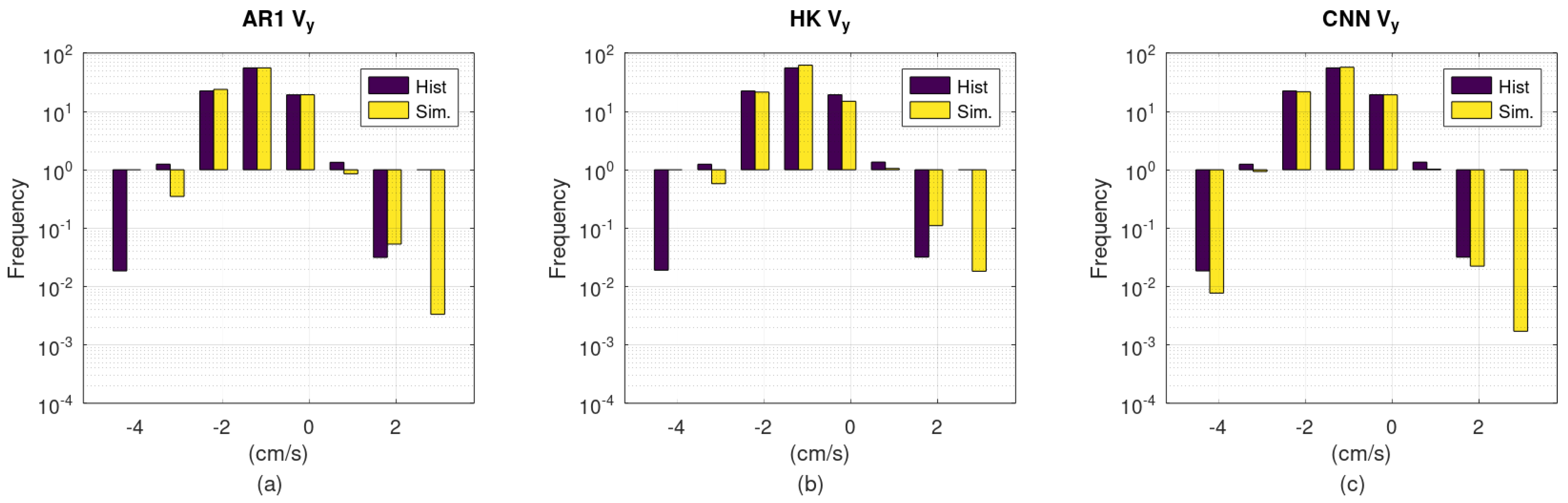
Figure 7, Figure 8 and Figure 9 compare histograms of the synthetic time series to those of the observed data. The y-axis is logarithmic; hence, longer downward bars correspond to lower frequencies. According to these figures, although all schemes reproduce the empirical distributions reasonably well, CNN presents a clear advantage regarding the extreme values.

Figure 10 shows the climacogram of ${\mathit{V}}_{\mathrm{x}}$. The reference climacogram initially exhibits a mild slope, which becomes steeper at larger scales. The AR1 scheme matches the reference at smaller scales but diverges at larger scales. The HK scheme shows a consistent deviation across all scales. The CNN scheme fits the reference climacogram closely across scales up to approximately 1000 time units.

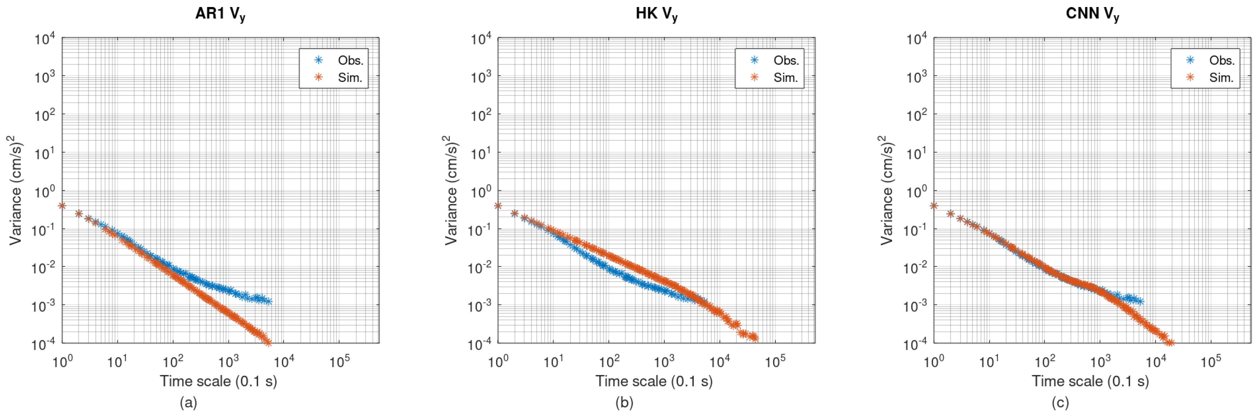
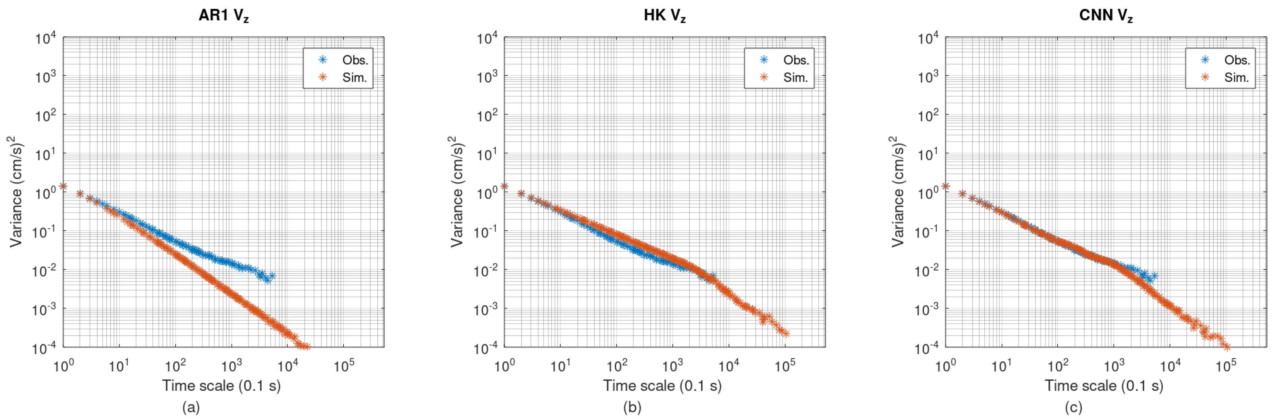
Figure 11 and Figure 12 show the climacograms of ${\mathit{V}}_{\mathrm{y}}$ and ${\mathit{V}}_{\mathrm{z}}$, respectively. In both cases, the reference climacograms follow a mild–steep–mild pattern across increasing scales. The AR1 scheme matches well at small scales but diverges significantly at larger ones. The HK scheme exhibits a mismatch at intermediate scales. In contrast, the CNN scheme replicates the reference climacograms well across all scales up to approximately 1000 time units.

4. Discussion

The results of the simulations suggest that all stochastic schemes performed generally well with respect to first-order statistics (mean, variance, and skewness). However, each scheme exhibited at least one shortcoming regarding second-order statistics (covariance, cross-covariance, and climacogram), which can be attributed to the theoretical foundations of the respective methods.

• Autoregressive order 1 (AR1): This scheme is well-suited for modeling Markovian processes, which exhibit scale-invariant variance at small scales, a feature manifested as a horizontal trend on the left side of their climacogram. This behavior aligns with the physical constraint of finite energy in natural systems, explaining AR1’s good performance at smaller scales. At larger scales, however, the variance of Markovian processes decays similarly to white noise, producing a climacogram slope of approximately $-1$. This fixed slope limits AR1’s capacity to capture long-range dependence or persistence in the data. Nevertheless, AR1 performs particularly well in preserving lag-1 cross-covariances. In general, autoregressive models preserve cross-covariances up to a lag equal to their order, as dictated by their mathematical formulation (see Equation (1)).
• Hurst–Kolmogorov (HK): This scheme models processes where the variance scales as a power law, resulting in a linear climacogram. However, such scaling implies an unrealistic increase in variance toward smaller scales, which would necessitate infinite energy (physically implausible for natural systems). As a result, the HK scheme may only align with the reference climacogram at specific ranges, that is, at lower scales (e.g., Figure 11b and Figure 12b), at higher scales, or it may exhibit a constant offset across all scales (e.g., Figure 10b). Additionally, the moving average weights in the HK scheme (derived from Equation (6)) are symmetric about the central weight, leading to symmetric cross-covariances—an assumption not generally met in empirical data.
• Convolutional neural network (CNN): Unlike the other two schemes, the CNN scheme is not based on explicit theoretical assumptions. Although it is mathematically equivalent to a moving average (MA) scheme, its weights are estimated heuristically rather than derived analytically, offering greater flexibility. A single convolutional layer is functionally equivalent to an MA scheme and can preserve persistence up to a time scale equal to the product of the time step $\mathrm{d}t$ and the number of weights used (i.e., $2J\mathrm{d}t$ in Equation (5)). In the present study, 1350 weights were used, implying that the CNN can preserve persistence up to 1350 time units. This is corroborated by Figure 10c, Figure 11c, and Figure 12c, which show excellent agreement between the CNN climacogram and the observed reference up to this scale.

Evidently, the CNN scheme outperformed the other two approaches in representing second-order statistics. In this case study, the matrices on the right-hand side of Equations (3) and (8) were positive definite, which made it possible to apply Equations (4) and (11) to compute the third moment of the white noise (i.i.d. terms) used in the AR1 and HK schemes. However, this favorable condition is not guaranteed in all applications. If the matrices are not positive definite, more advanced methods, such as solving an optimization problem, are required for the AR1 and HK schemes to preserve the observed skewness [31].

The synthetic time series generated by the AR1 scheme produced a realistic climacogram at smaller scales, but its fixed slope of $-1$ at larger scales limits its suitability for processes with long-range dependence. The HK scheme used here is capable of modeling climacograms with arbitrary, but constant, slopes across all scales. More sophisticated variants, such as the filtered Hurst–Kolmogorov model, can yield climacograms with more realistic behavior at both low and high scales, although deriving the moving average weights in such models is considerably more complex than directly applying Equation (6). The CNN-based scheme, by contrast, can reproduce the shape of any climacogram up to a scale corresponding to the kernel size (expressed in time units, where each unit equals the time step of the series). In the present case study, it is noteworthy that CNN was the only scheme that successfully replicated the climacogram of the observed ${\mathit{V}}_{\mathrm{y}}$ component. The form of this climacogram suggests the presence of a trend in the original data, the origin of which remains unclear; it may result from the pump motor in the hydraulic experiment setup or from artifacts introduced by the ADV’s electronics. Regardless of the source, CNN managed to reproduce this feature accurately.

A disadvantage of CNN-based schemes is the computational cost associated with training. In this case, training required approximately 30 min on a 2.5 GHz dual-core CPU. This duration can be significantly reduced by leveraging multi-core architectures, and even more so by using a GPU instead of a CPU.

5. Conclusions

This study introduced a novel machine learning-based stochastic simulation scheme utilizing a single convolutional neural network (CNN) layer as a generator. In contrast to the commonly used generative adversarial networks (GANs), which require a more complex generator–discriminator framework, the proposed approach simplifies the architecture by employing a custom-designed cost function. This function directly compares essential statistical properties between observed and synthetic time series, thereby removing the need for a discriminator.

The effectiveness of the CNN-based scheme was evaluated against conventional stochastic methods designed for Markovian and Hurst–Kolmogorov processes. The results demonstrated that the CNN-based approach outperforms these traditional methods in reproducing second-order statistics. Notably, it preserved variance across temporal scales and successfully captured the effects of persistence, both critical for producing realistic long-term simulations.

Furthermore, by establishing the formulation equivalence between the CNN-based generator and classical moving average schemes, this study highlighted both the theoretical implications and certain limitations of the method. A key advantage of the proposed scheme lies in its simplicity and practical applicability—it can be implemented in widely accessible tools such as standard spreadsheet software. This makes it a valuable option for engineers and practitioners involved in design, planning, and decision-making processes.