
Regional Frequency Analysis Using L-Moments for Determining Daily Rainfall Probability Distribution Function and Estimating the Annual Wastewater Discharges

 ,
,  , , and
Abstract
1. Introduction
2. Materials and Methods
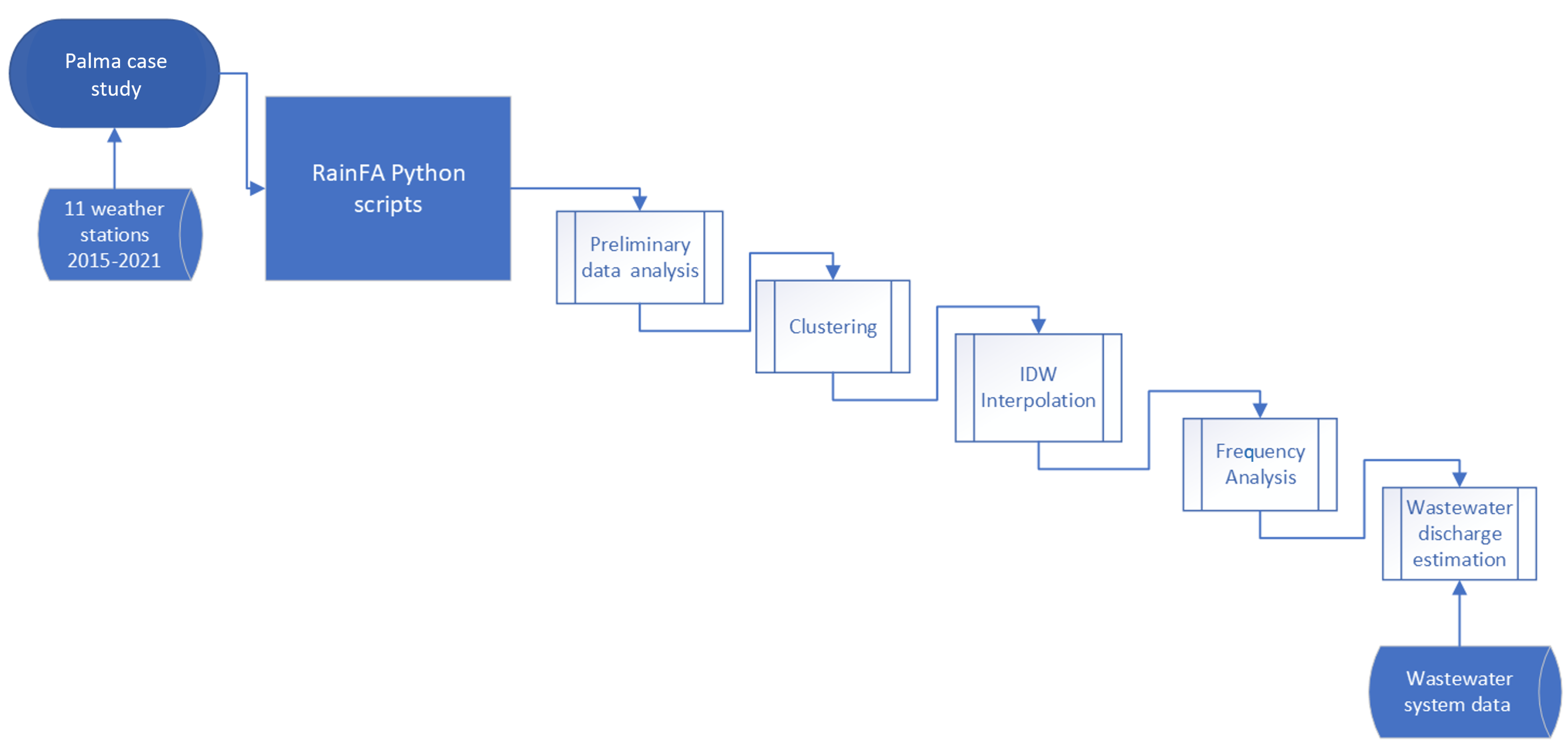
2.1. RainFA
2.2. Preliminary Data Analysis
2.2.1. Temporal Homogenization
2.2.2. Daily Quality Control
User-Defined Thresholds
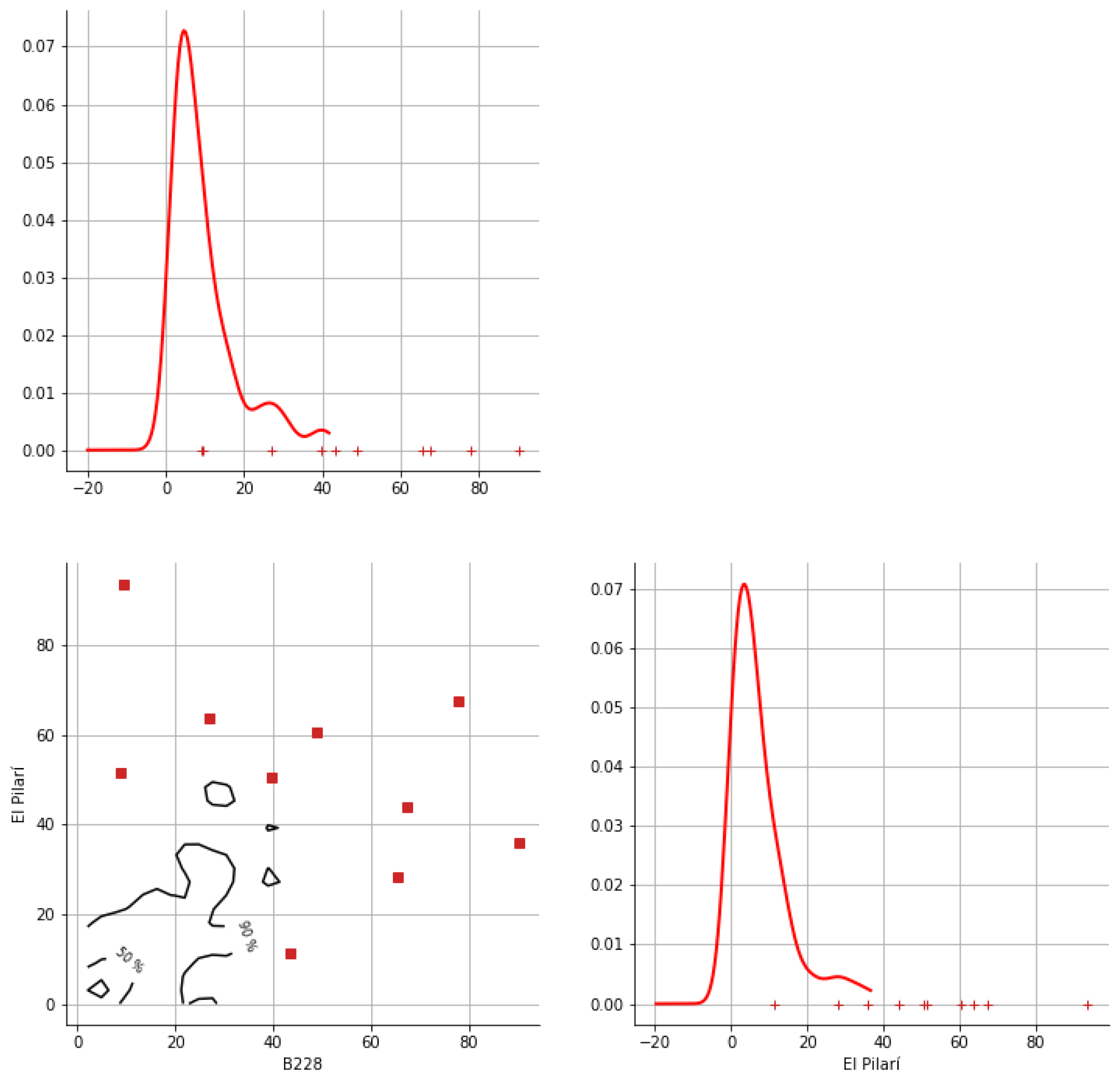
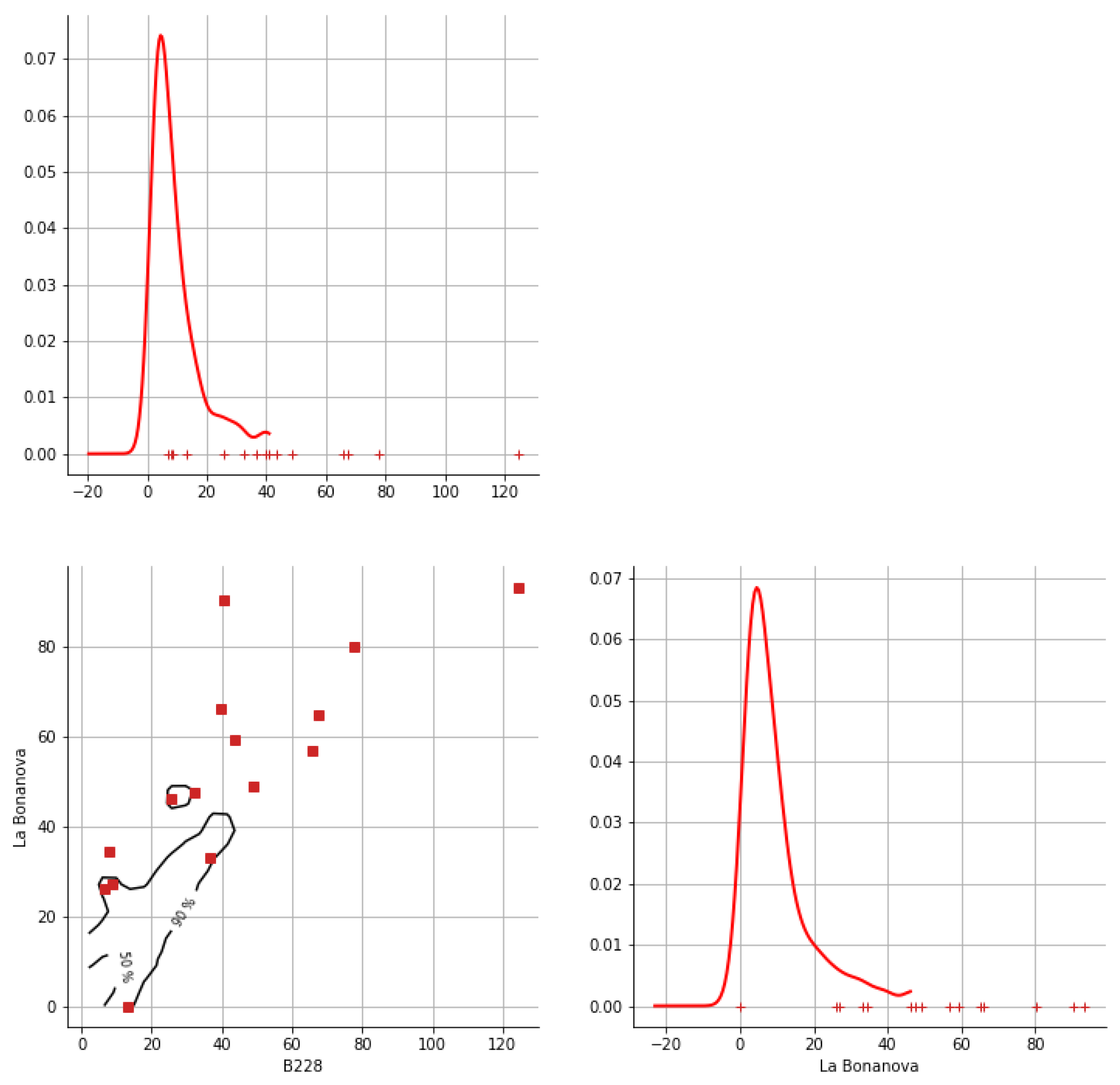
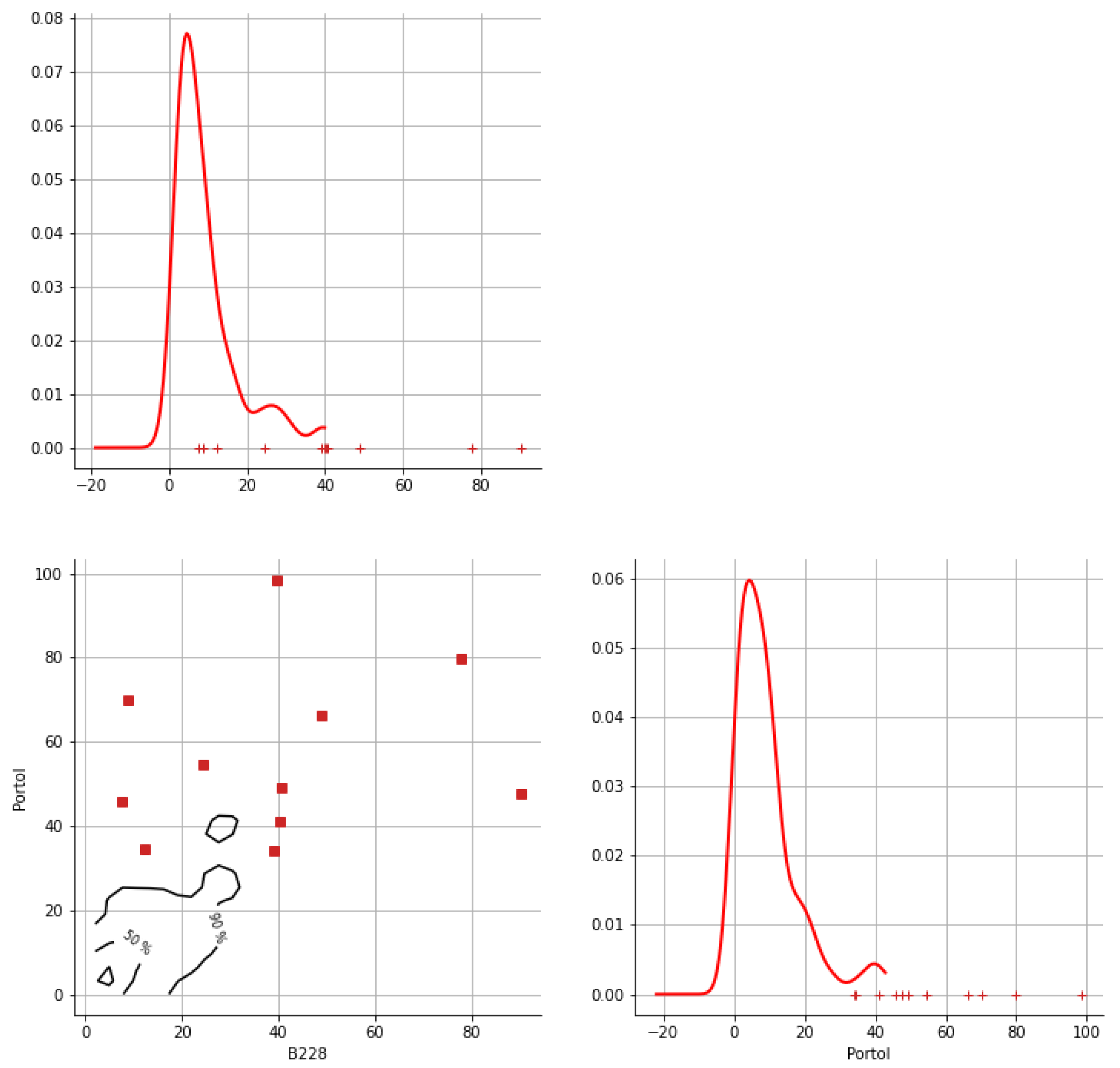
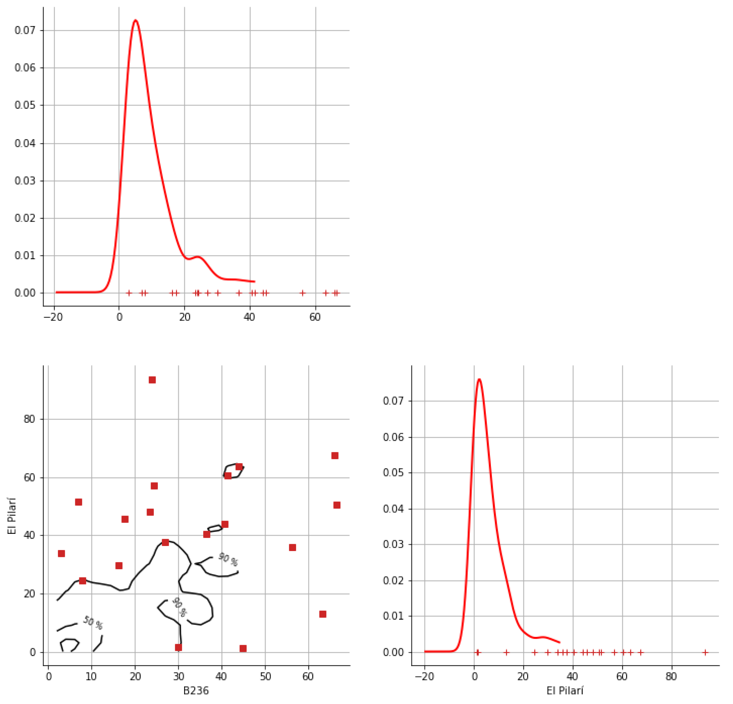
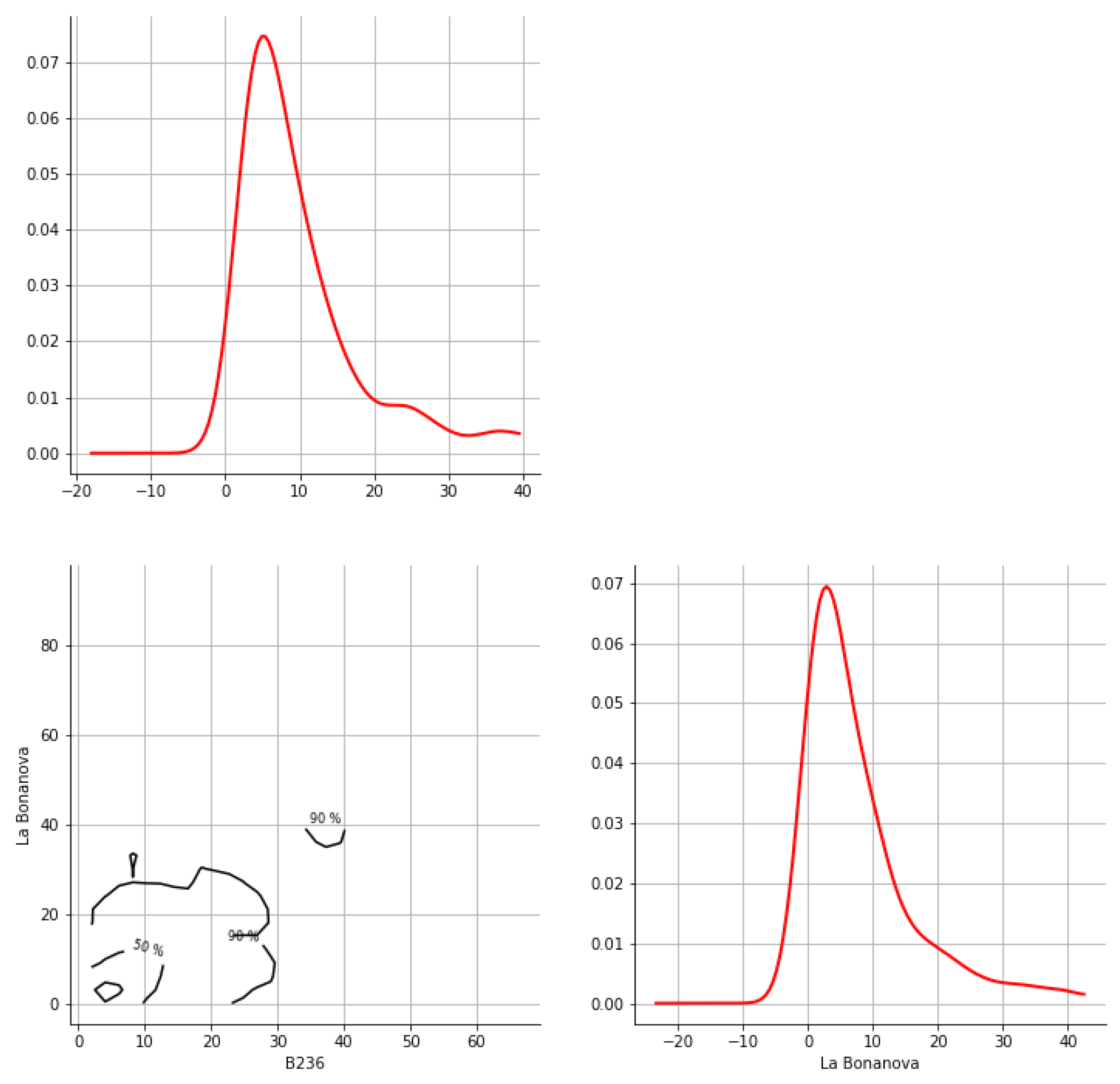
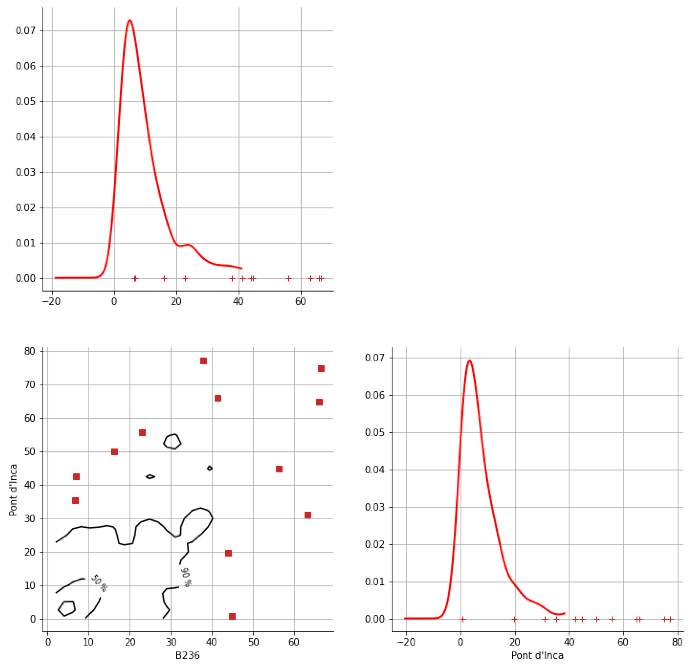
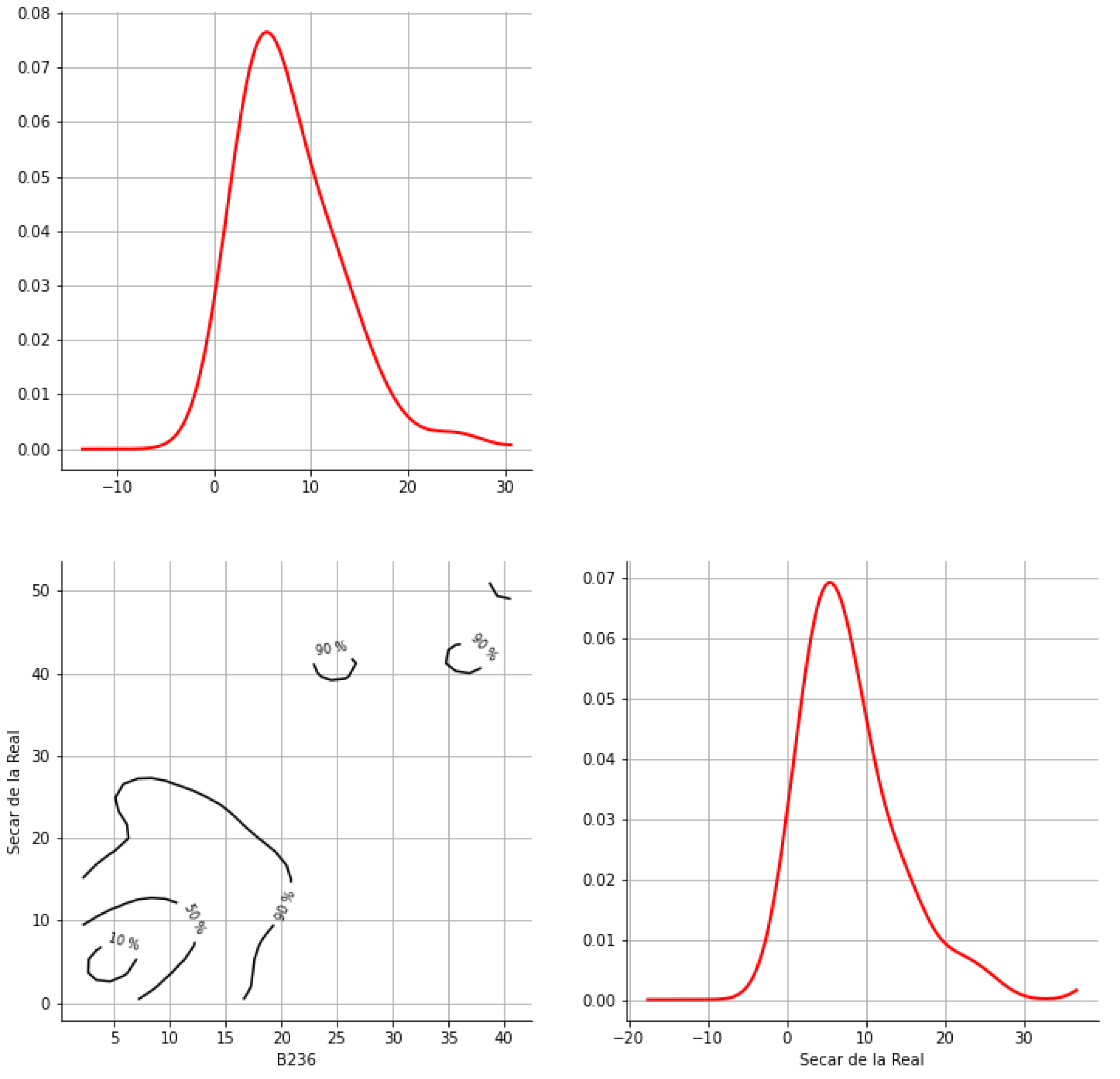
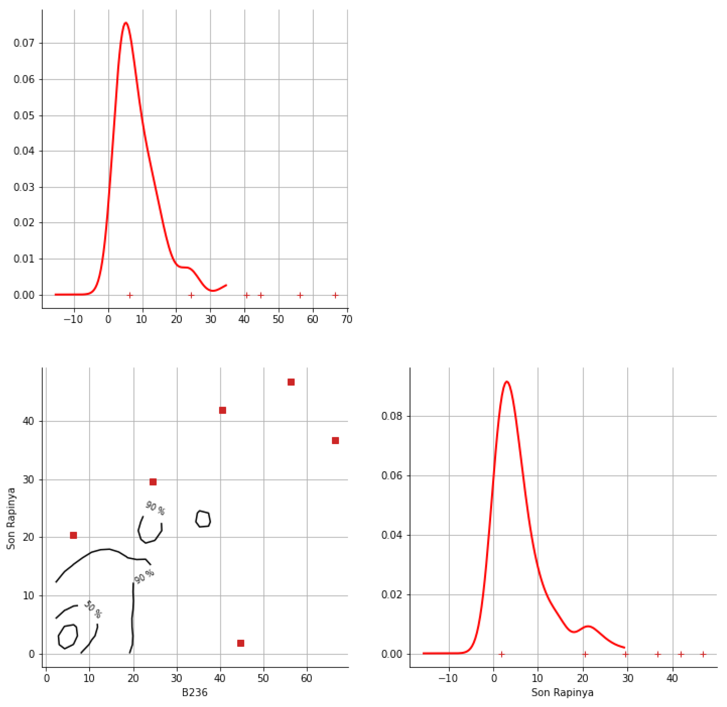
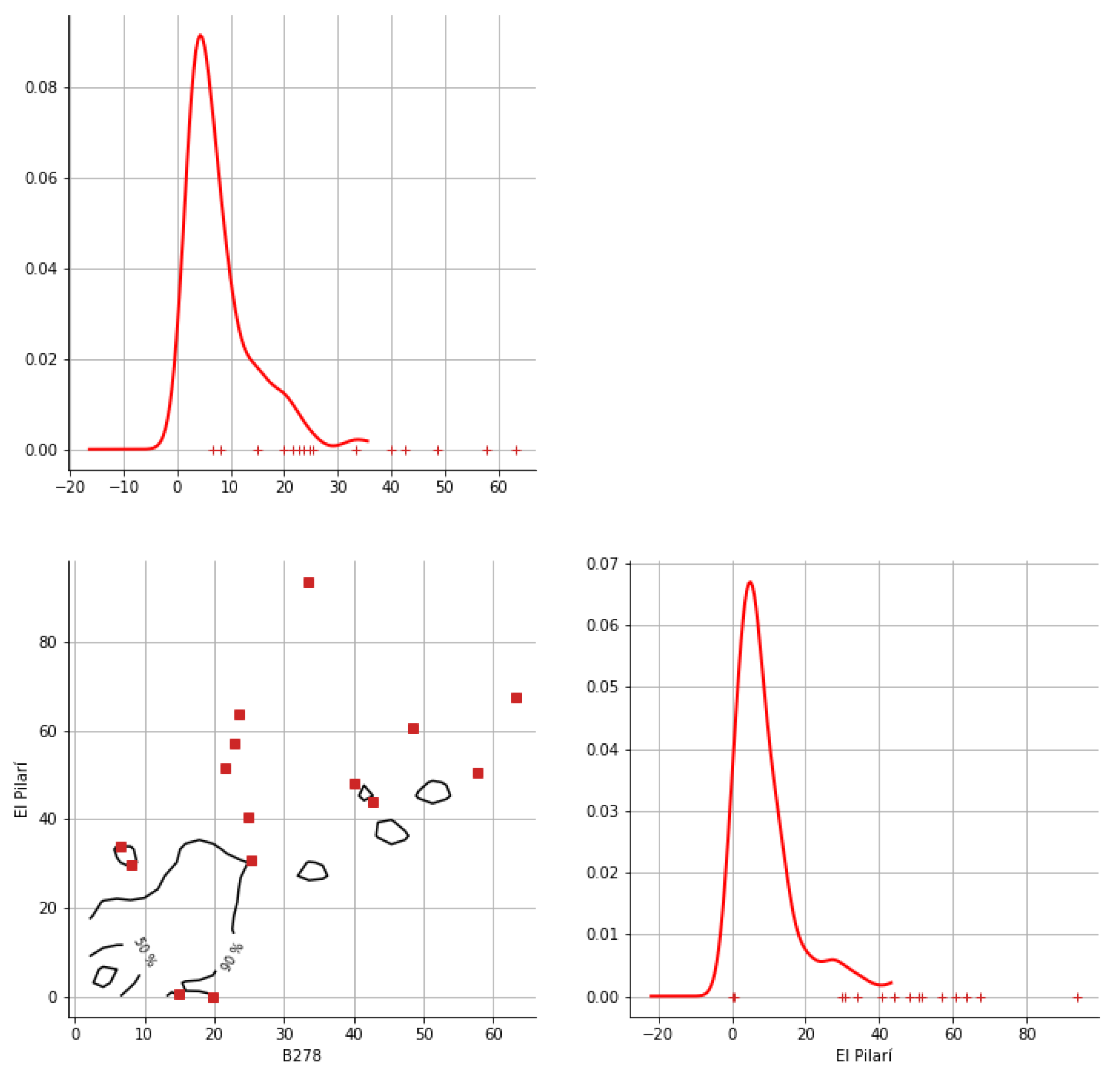
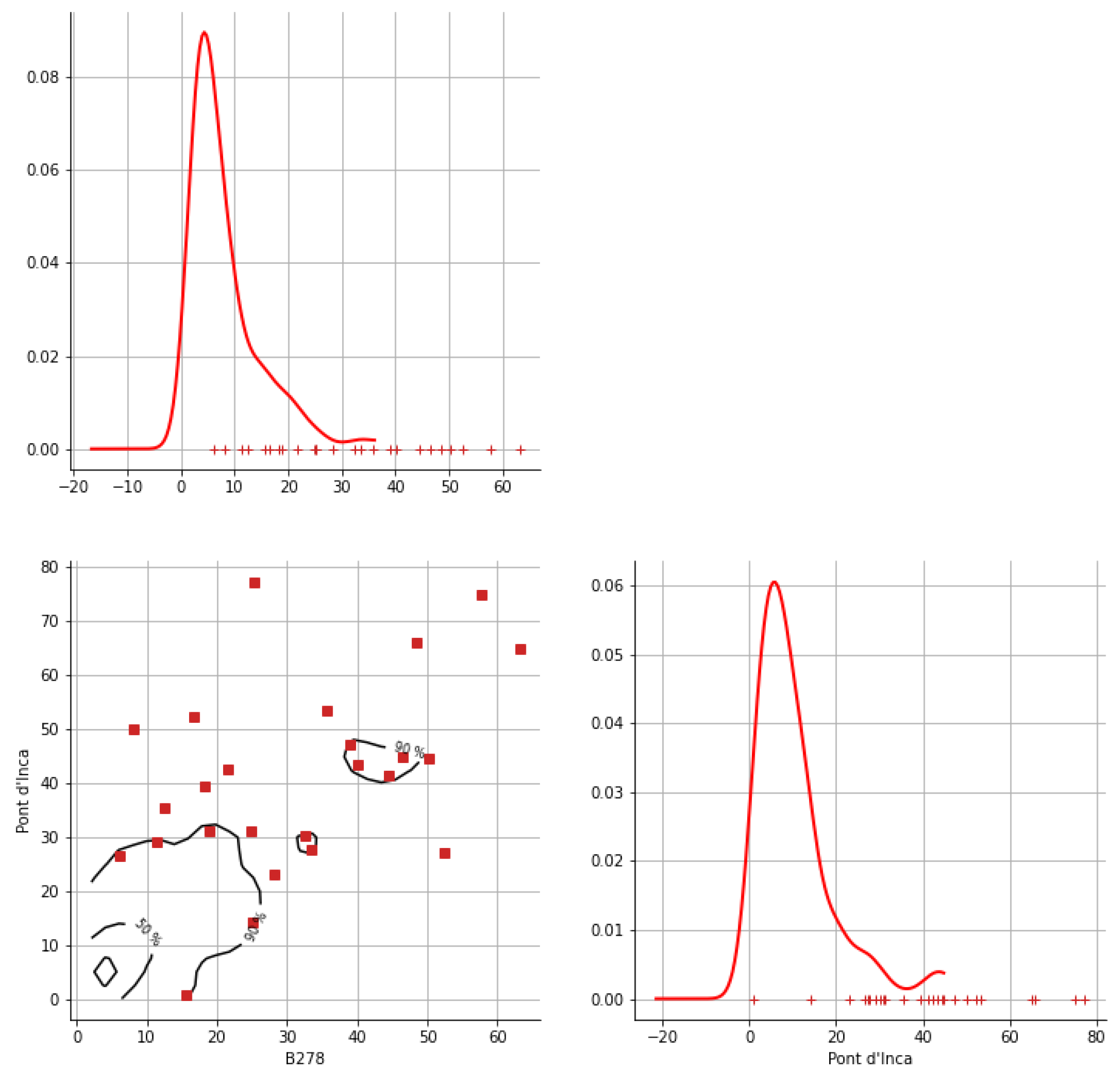
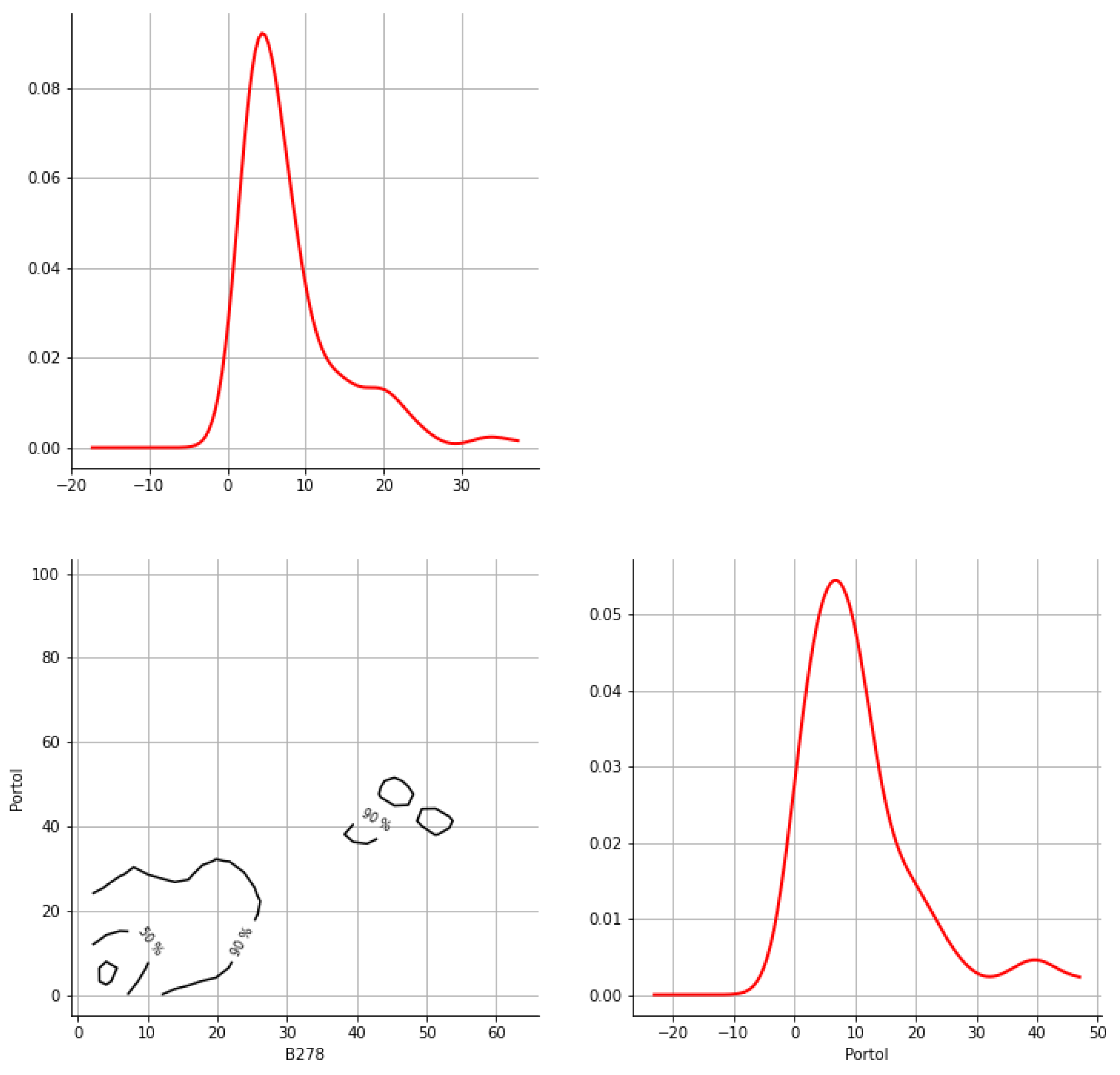
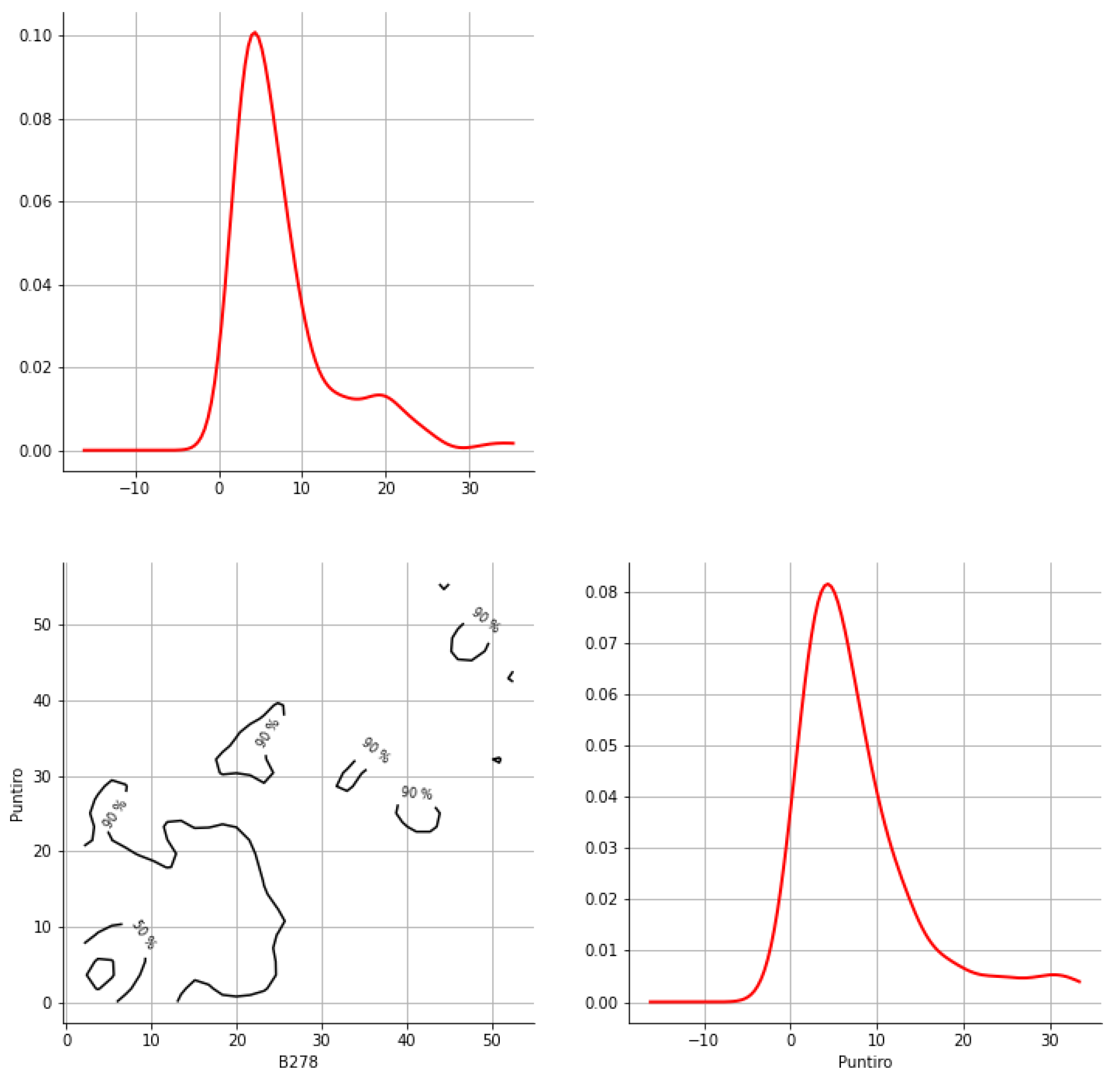
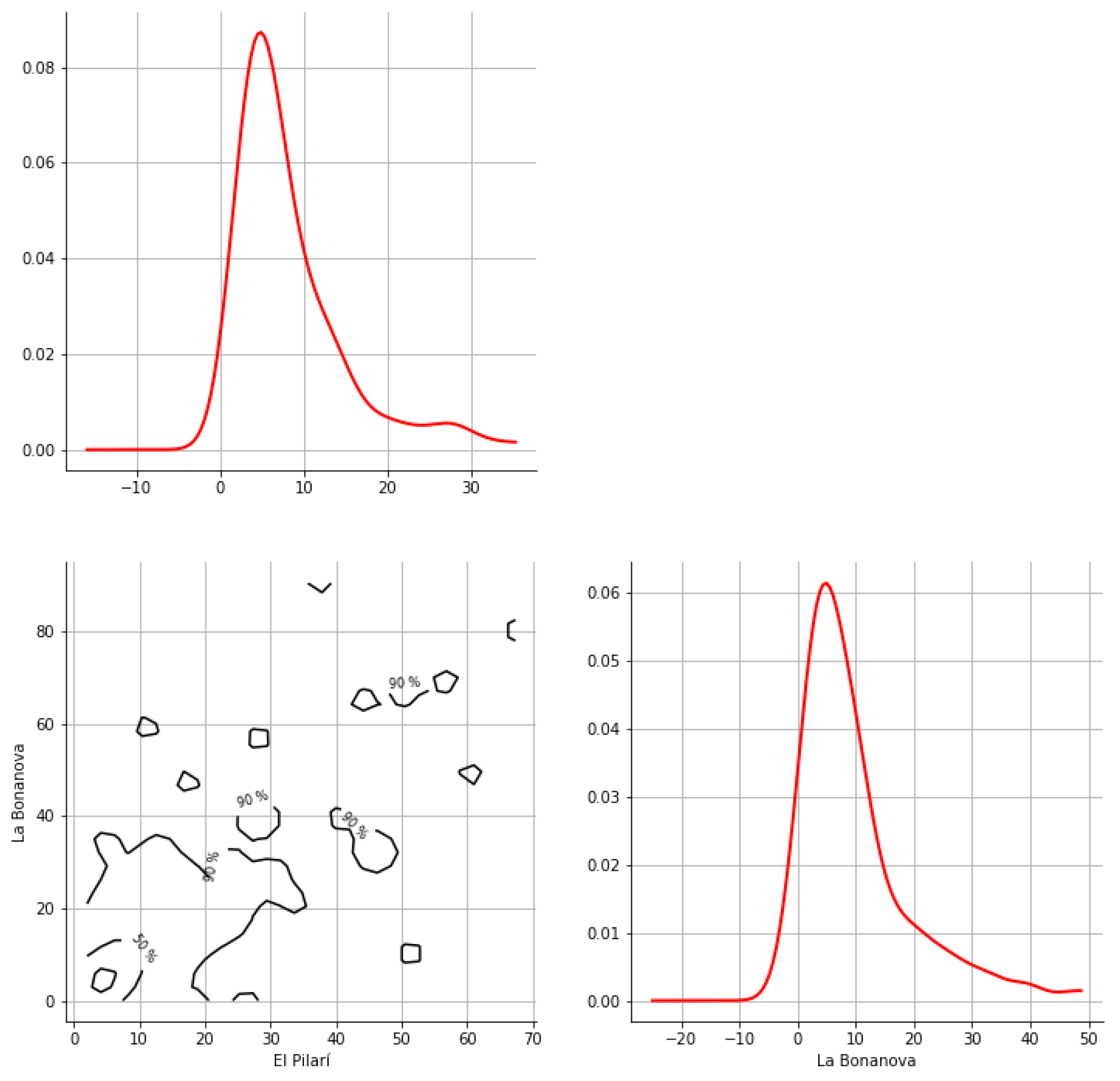
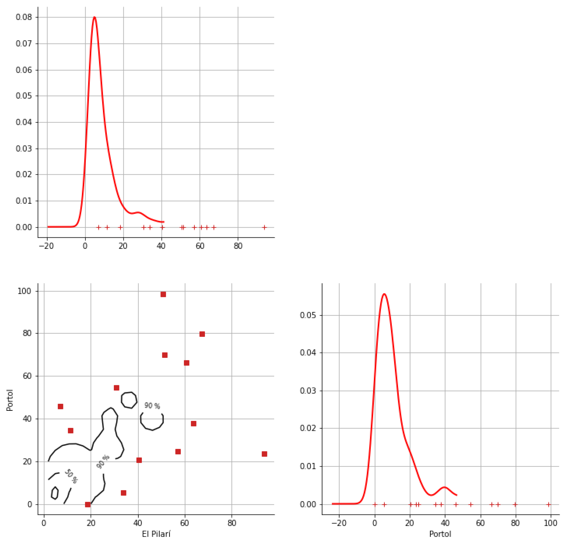
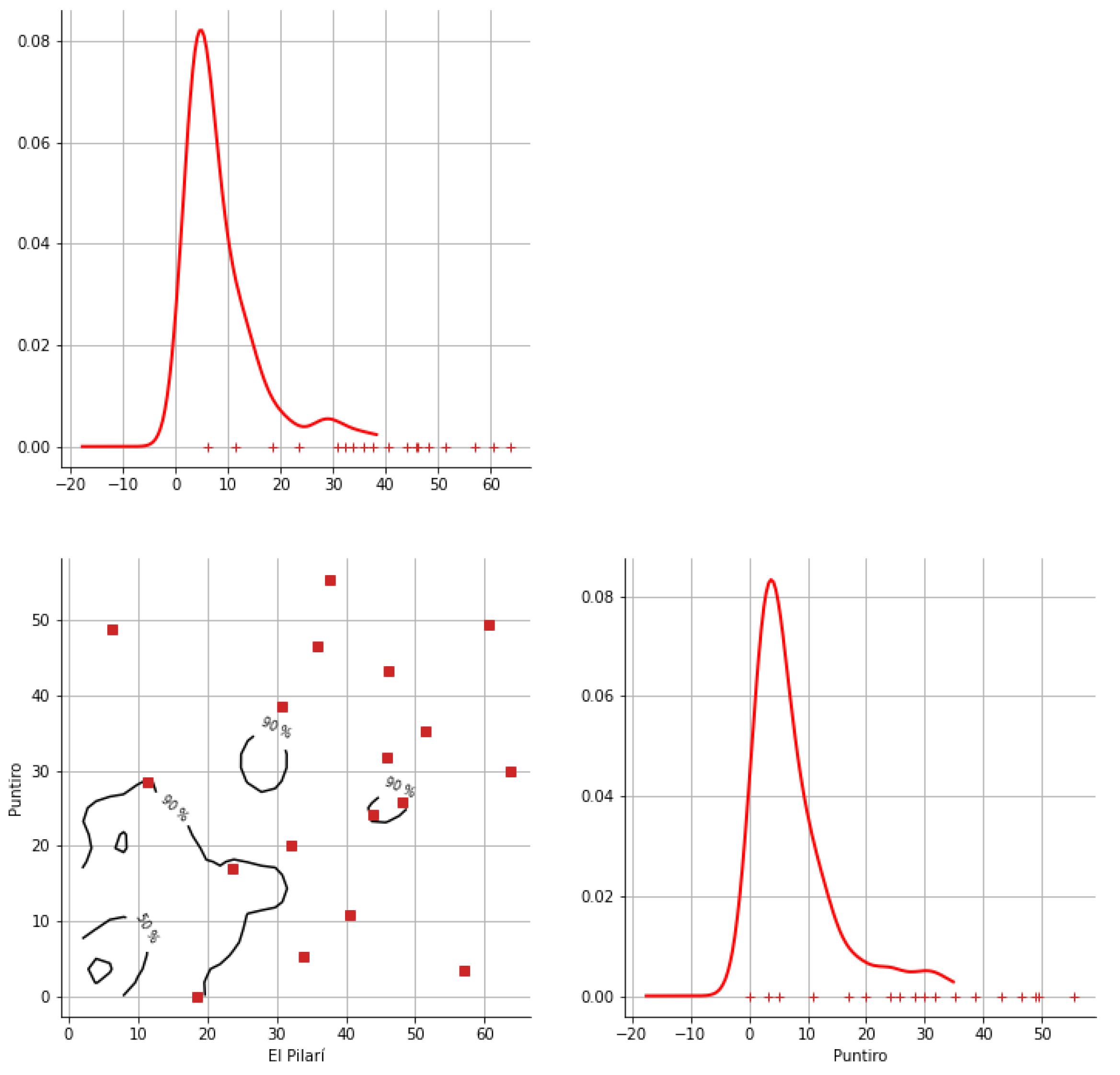
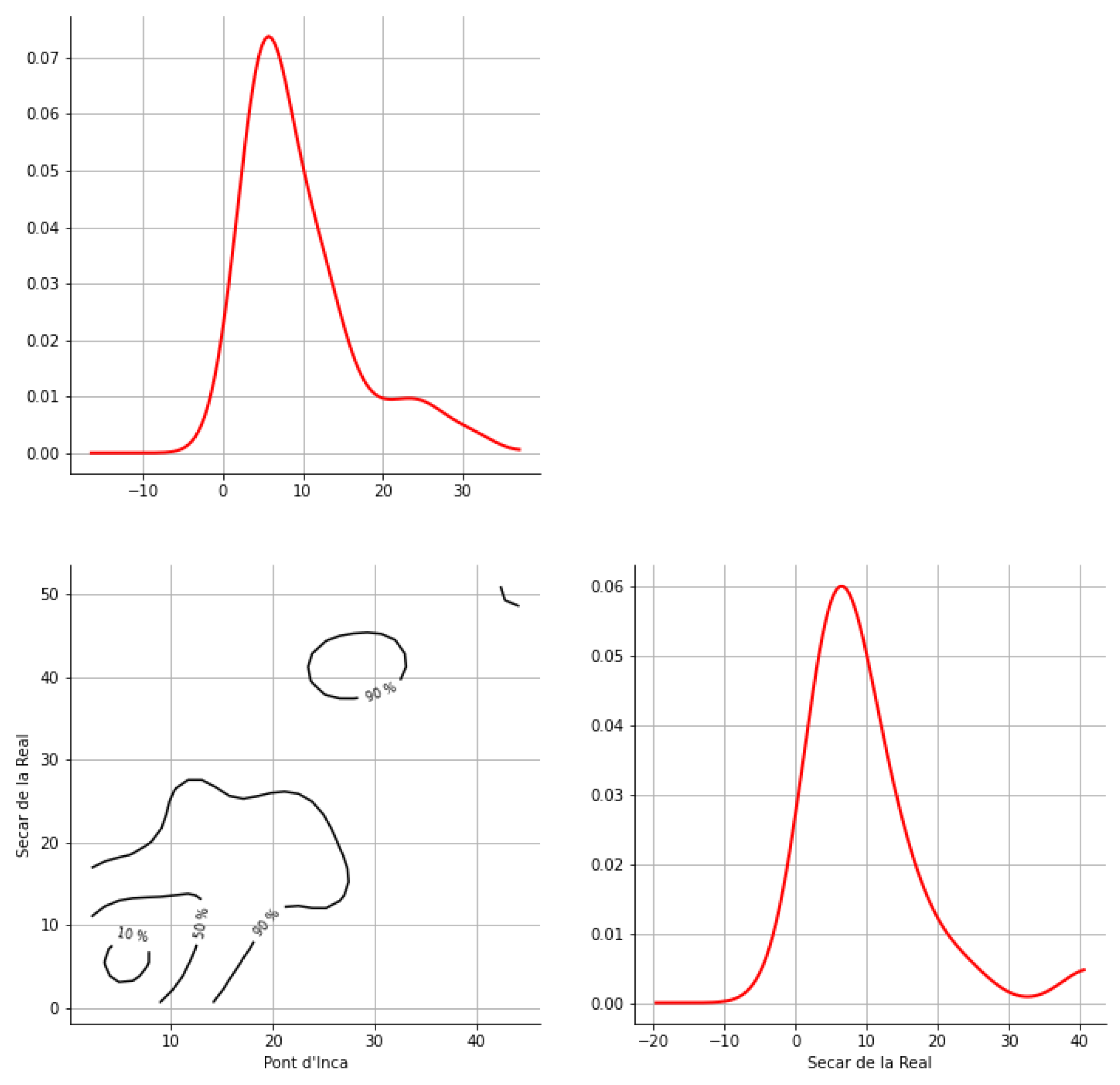
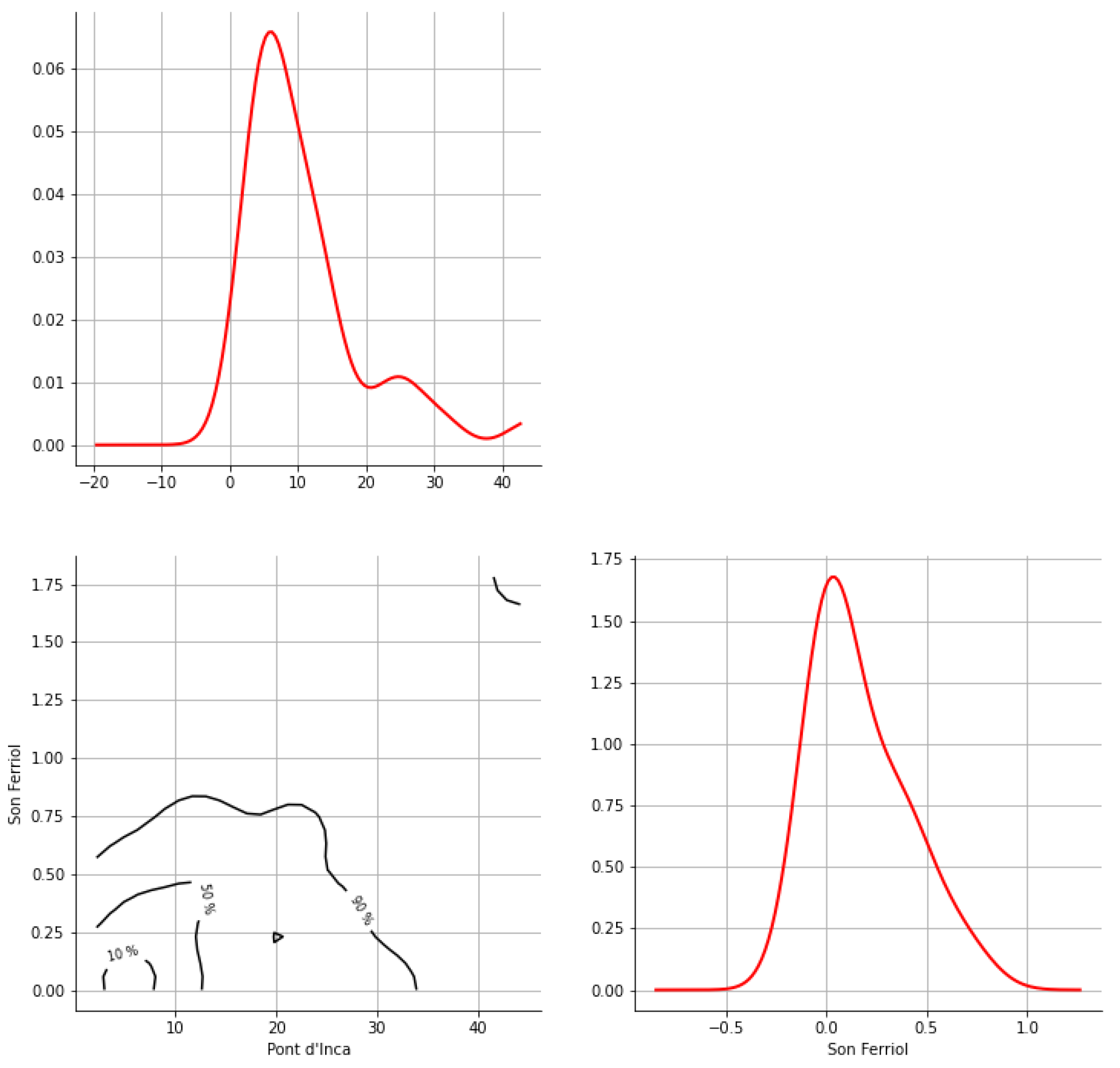
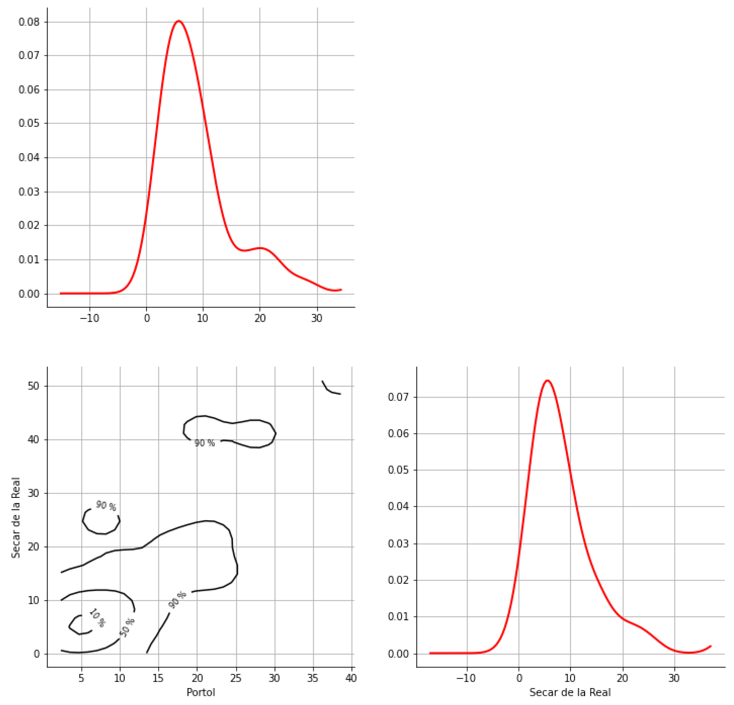
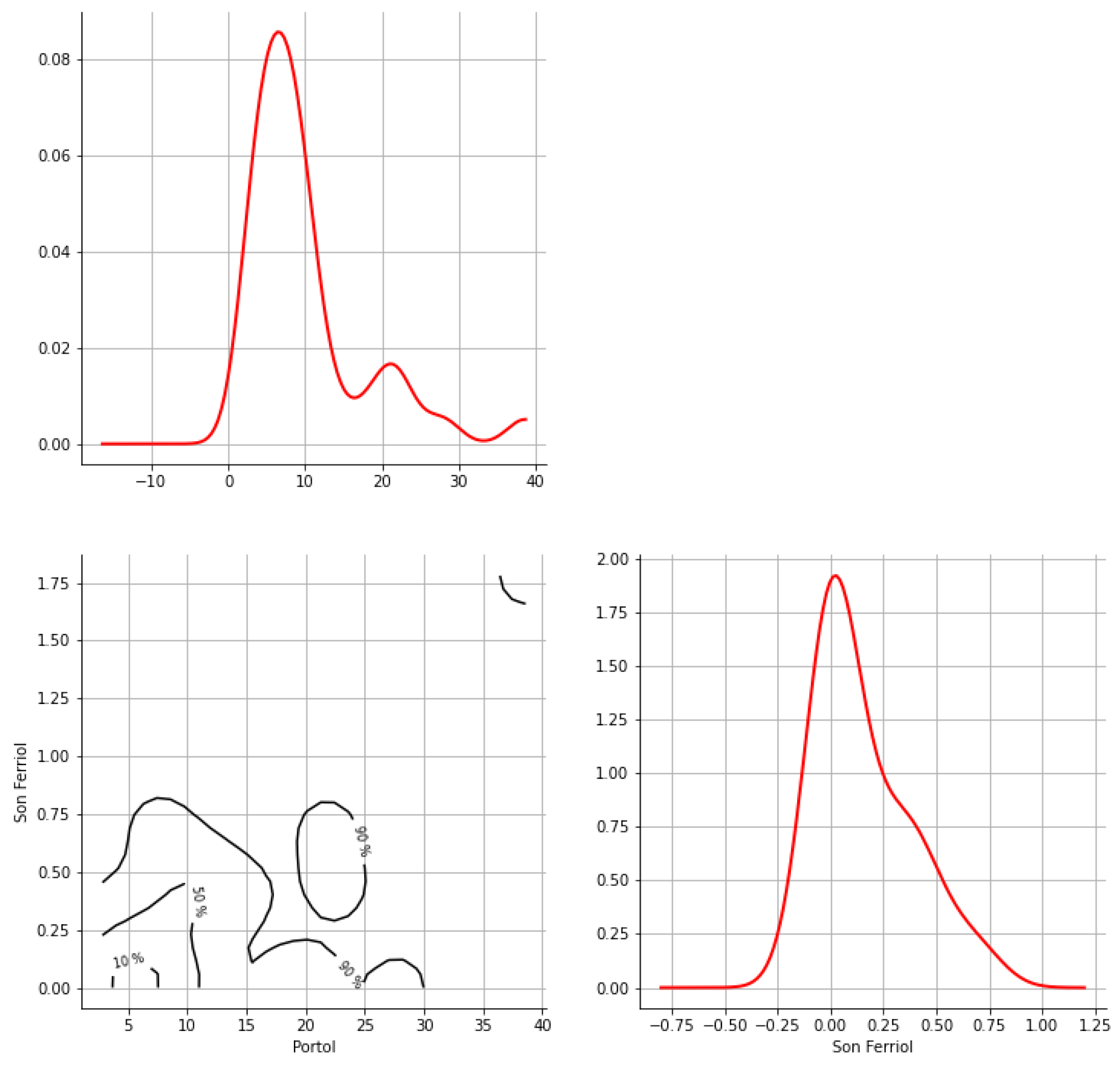
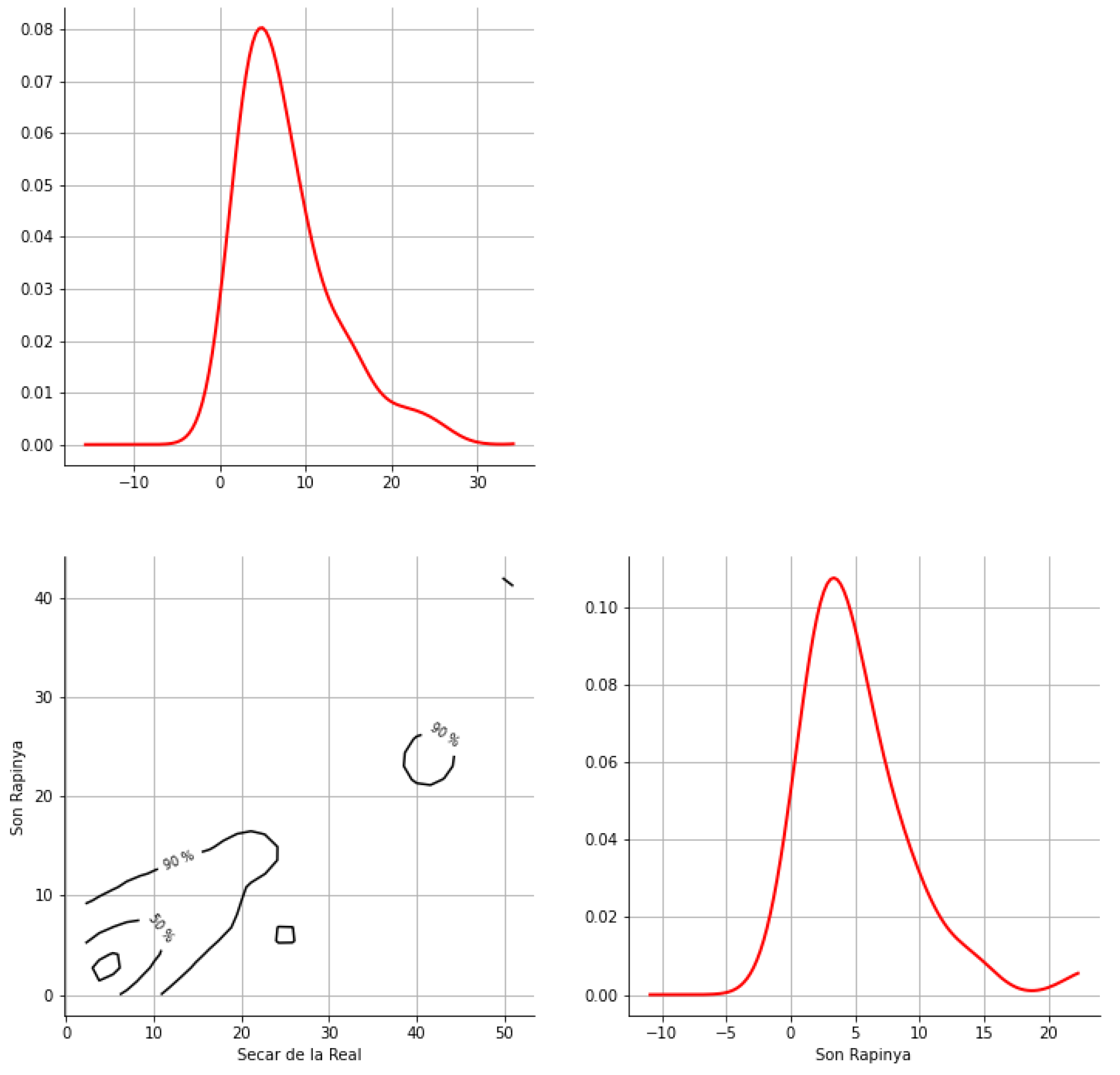
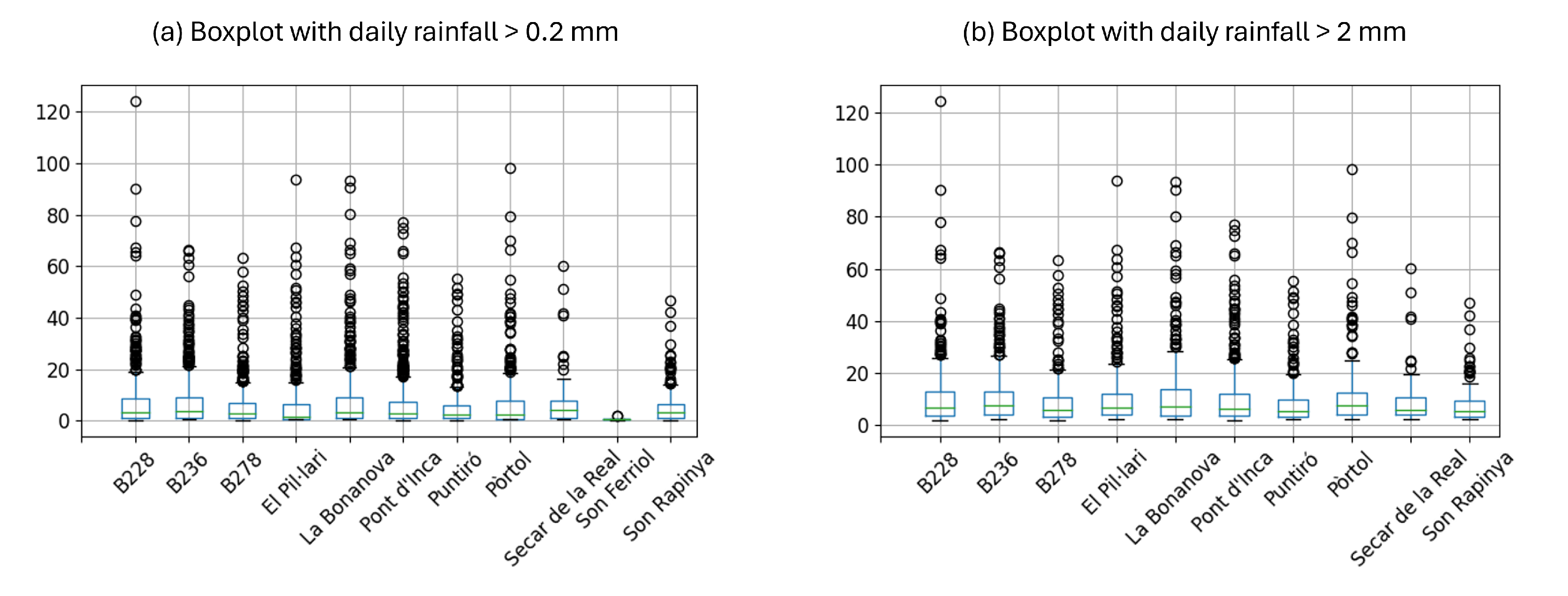
Outlier Detection and Bivariate HDR Boxplots
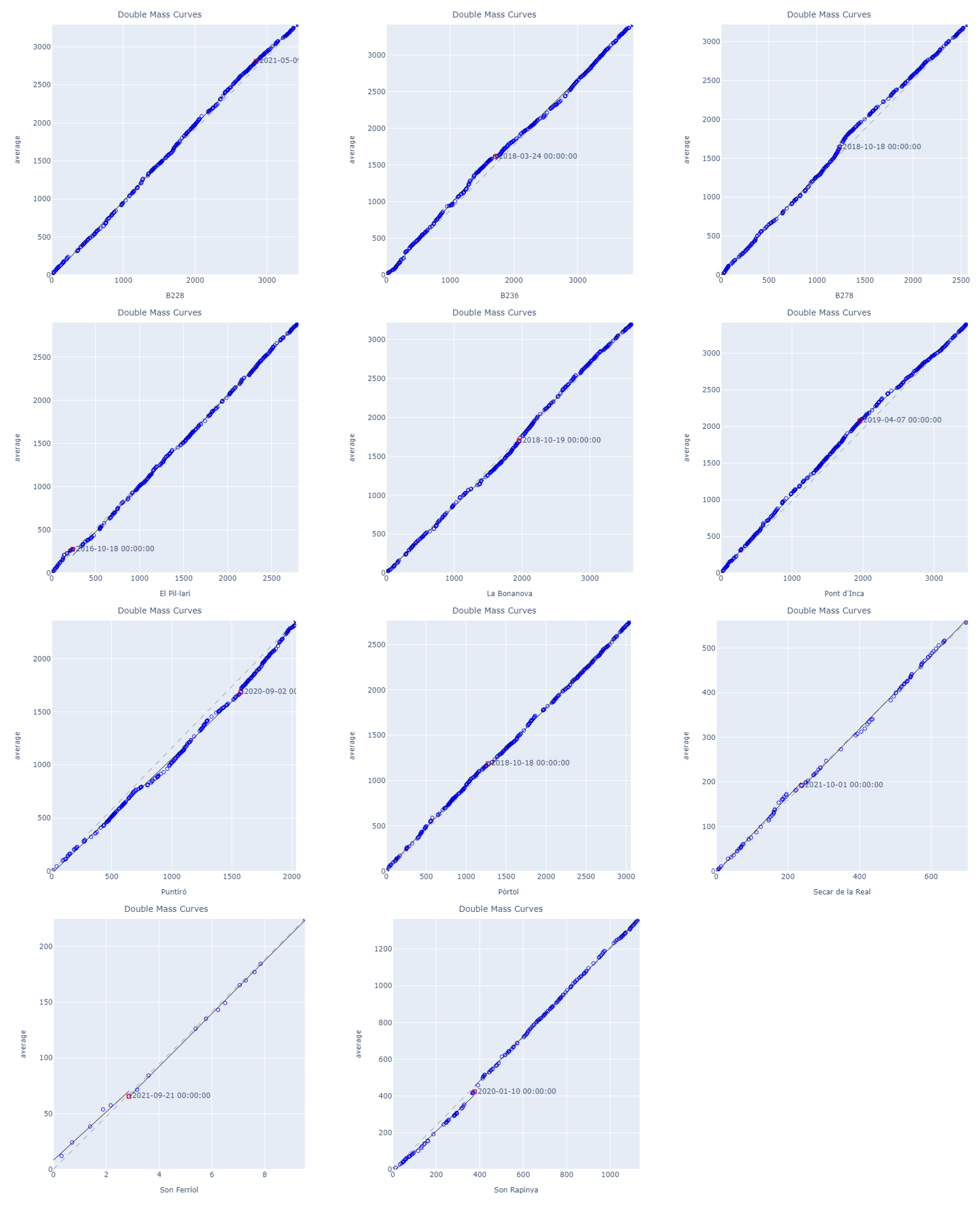
Double-Mass Curves
Trend Analysis
2.3. Identification of Candidate Homogeneous Regions
2.3.1. Cluster Overview
2.3.2. Cluster Optimization
2.3.3. Ward’s Dendrogram
2.3.4. L-Moments Homogeneity Measure
2.4. Generalized IDW Interpolation for Homogeneous Regions
2.5. Probability Distribution Functions Selection for Homogeneous Regions
2.6. Evaluation Criteria
2.6.1. Detection of Occurrence of Rainfall
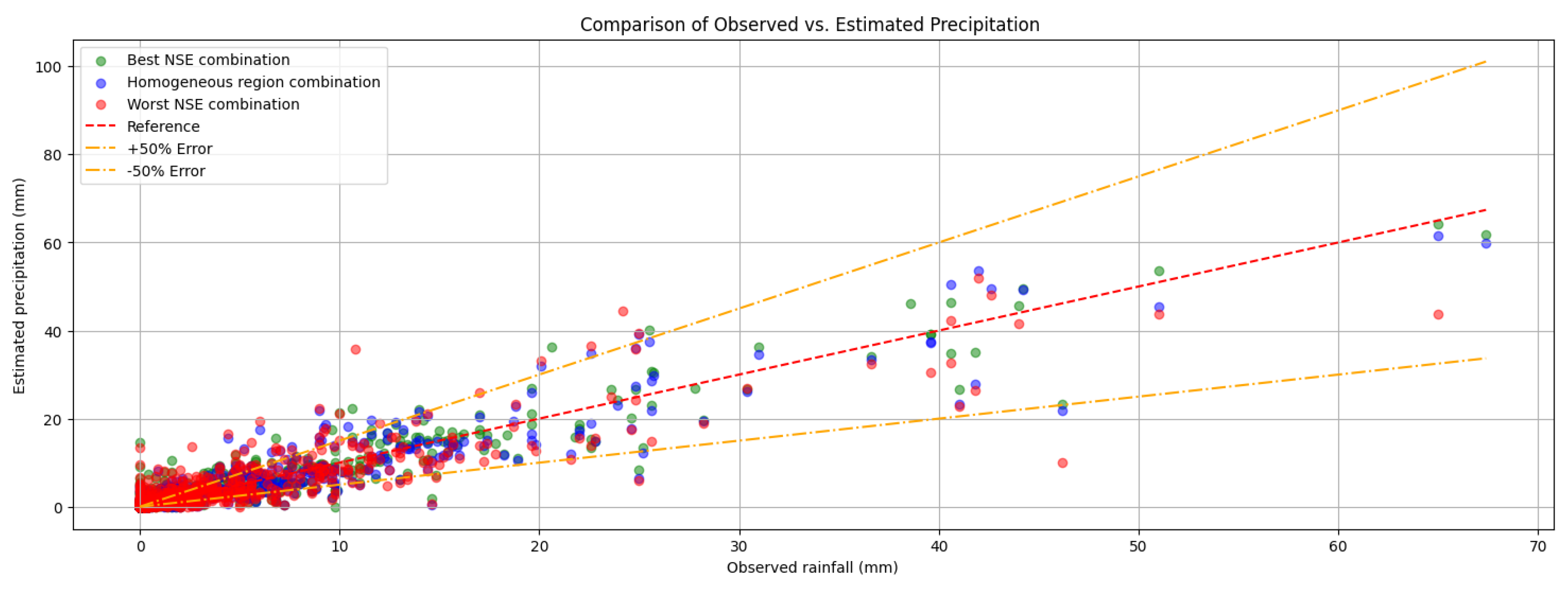
2.6.2. Accuracy of the Simulations
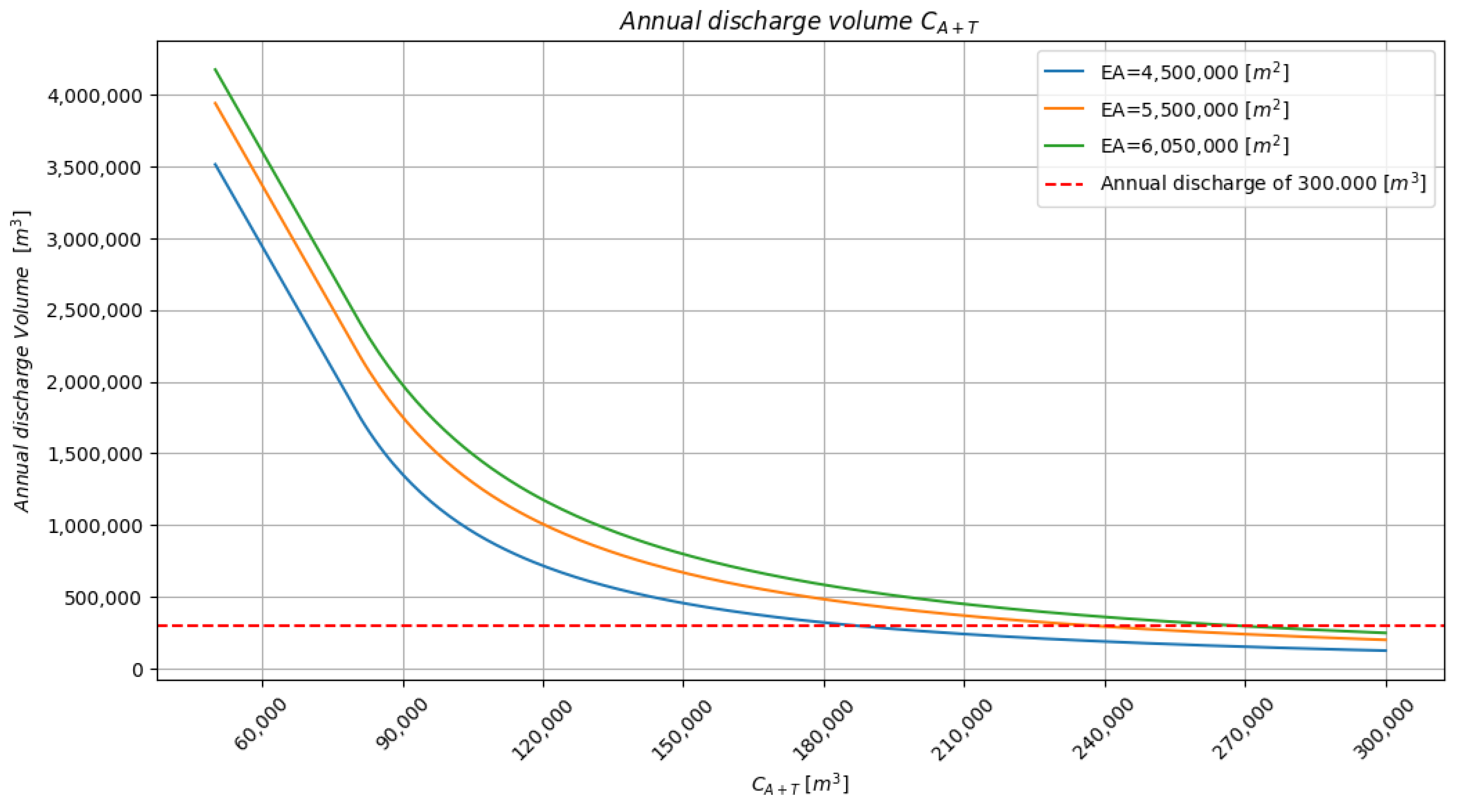
2.7. Annual Sewage Discharge Estimation
- •
- Effective Area (EA): non-permeable area in the watershed.
- •
- Rainfall Inflow (): total rainfall entering the system for the event j of the year i. .
- •
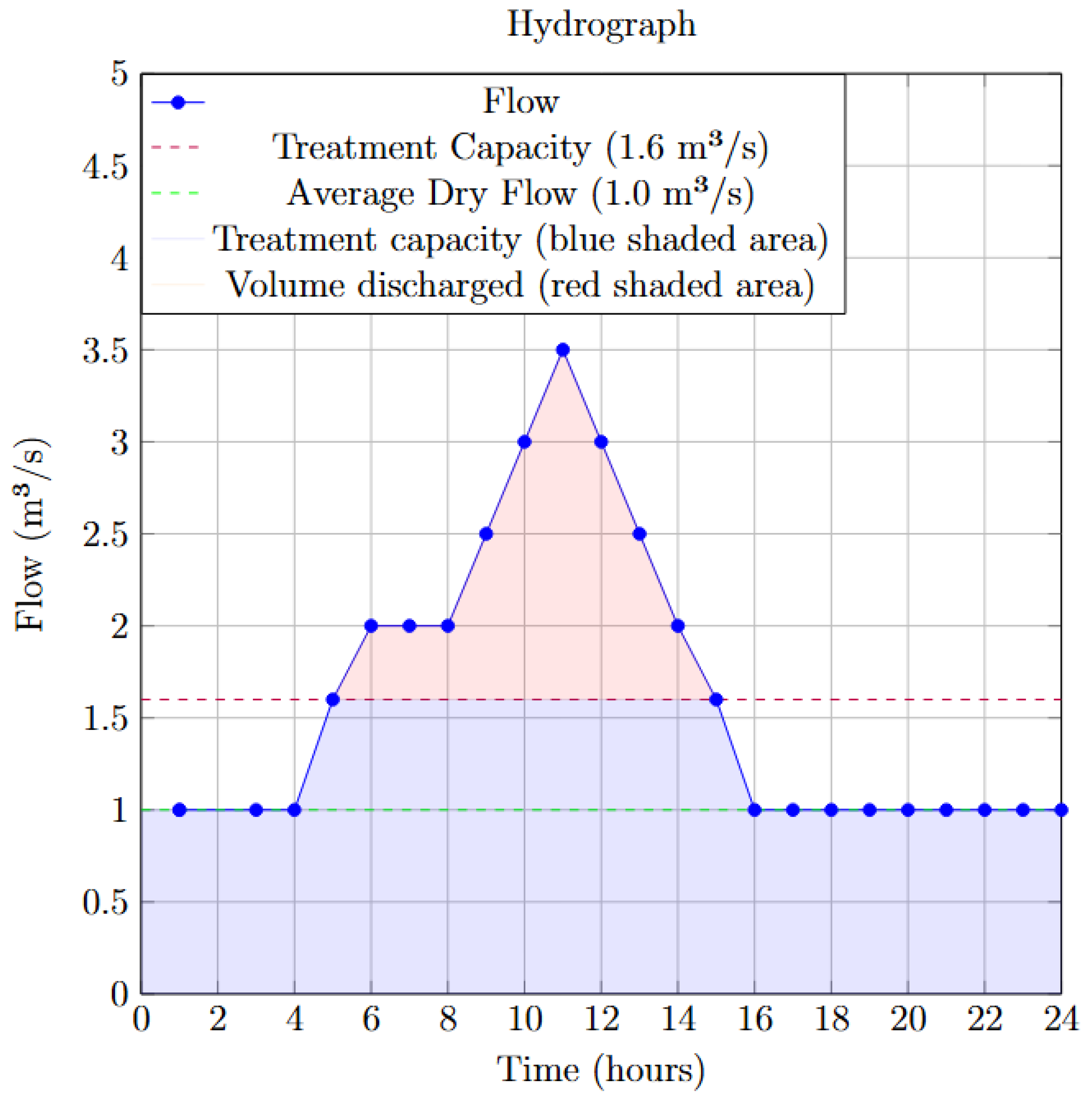
- Attenuation and Treatment Capacity (): defined as the sum of the volume of the sewer system and attenuation tanks (), and the capacity volume of the treatment plant (). The parameter depends on the duration of the rainfall, as shown in Figure 2.
- •
- Dry Volume (): average daily volume of wastewater during dry days.
- •
- Discharge event (): discharge for the event when the attenuation and treatment capacity is exceeded.

3. Description of the Study Area and Data Sources
3.1. Case Study
3.2. Data Sources
4. Results
4.1. Data Curation and Stationarity
4.2. Clustering and Homogeneity
4.3. Evaluation of the Precipitation Inference Model Using the IDW Method in the Selected Homogeneous Region
4.3.1. Detection of Occurrence of Rainfall
4.3.2. Accuracy of Rainfall
4.4. PDF Selection
4.5. Sewage Discharge Estimation
5. Discussion
6. Conclusions
Author Contributions
Funding
Institutional Review Board Statement
Informed Consent Statement
Data Availability Statement
Acknowledgments
Conflicts of Interest
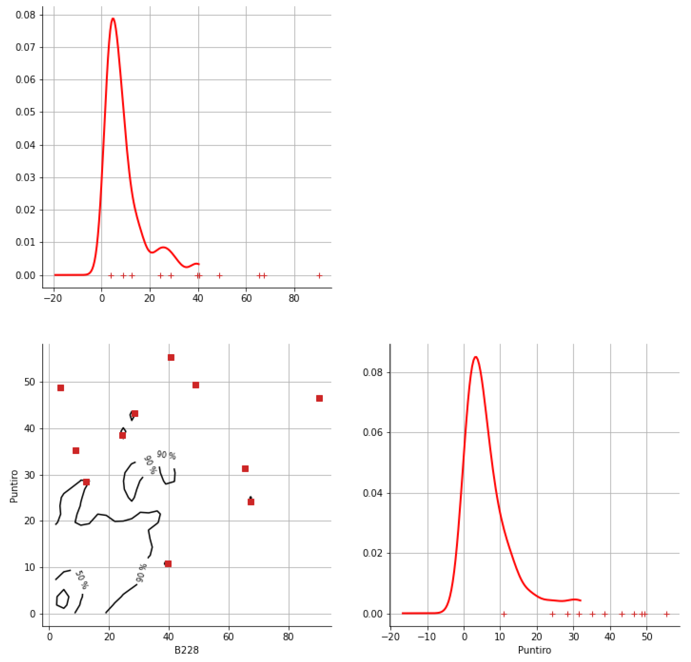
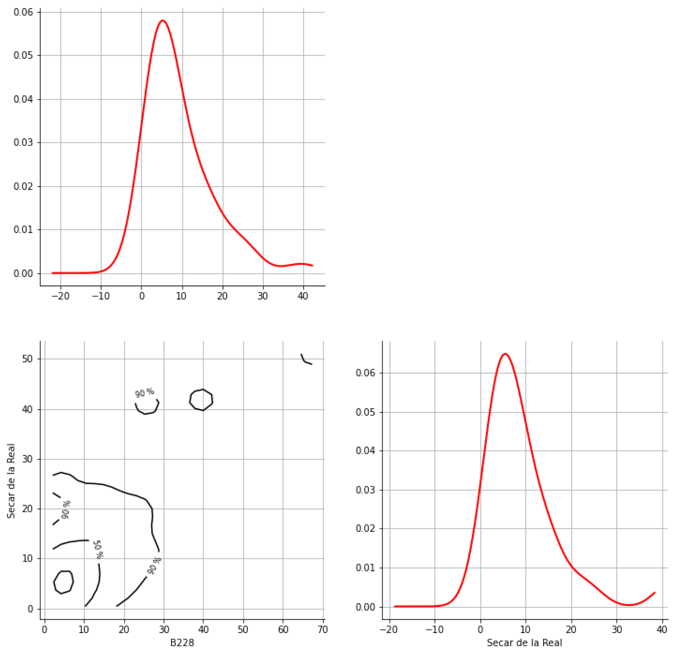
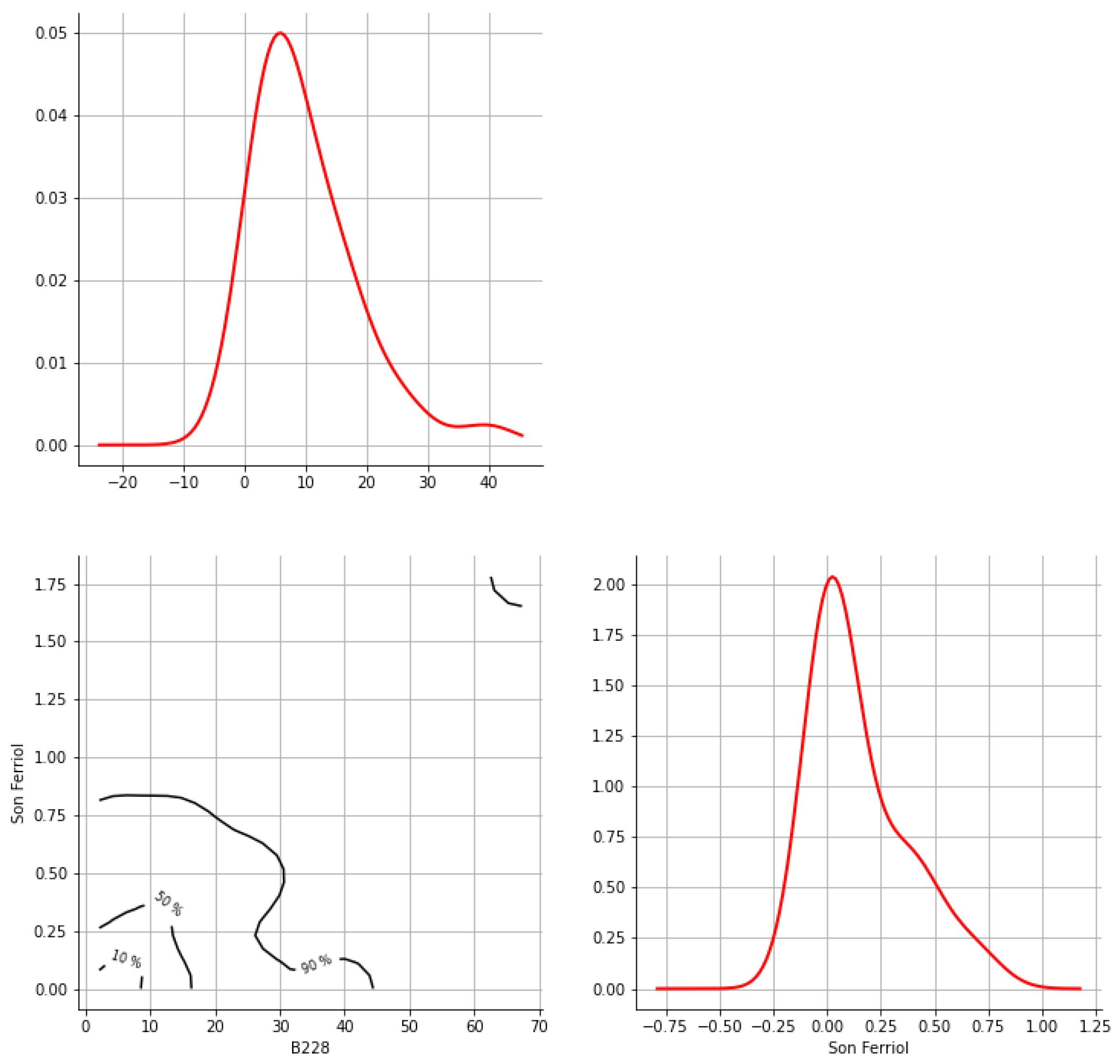
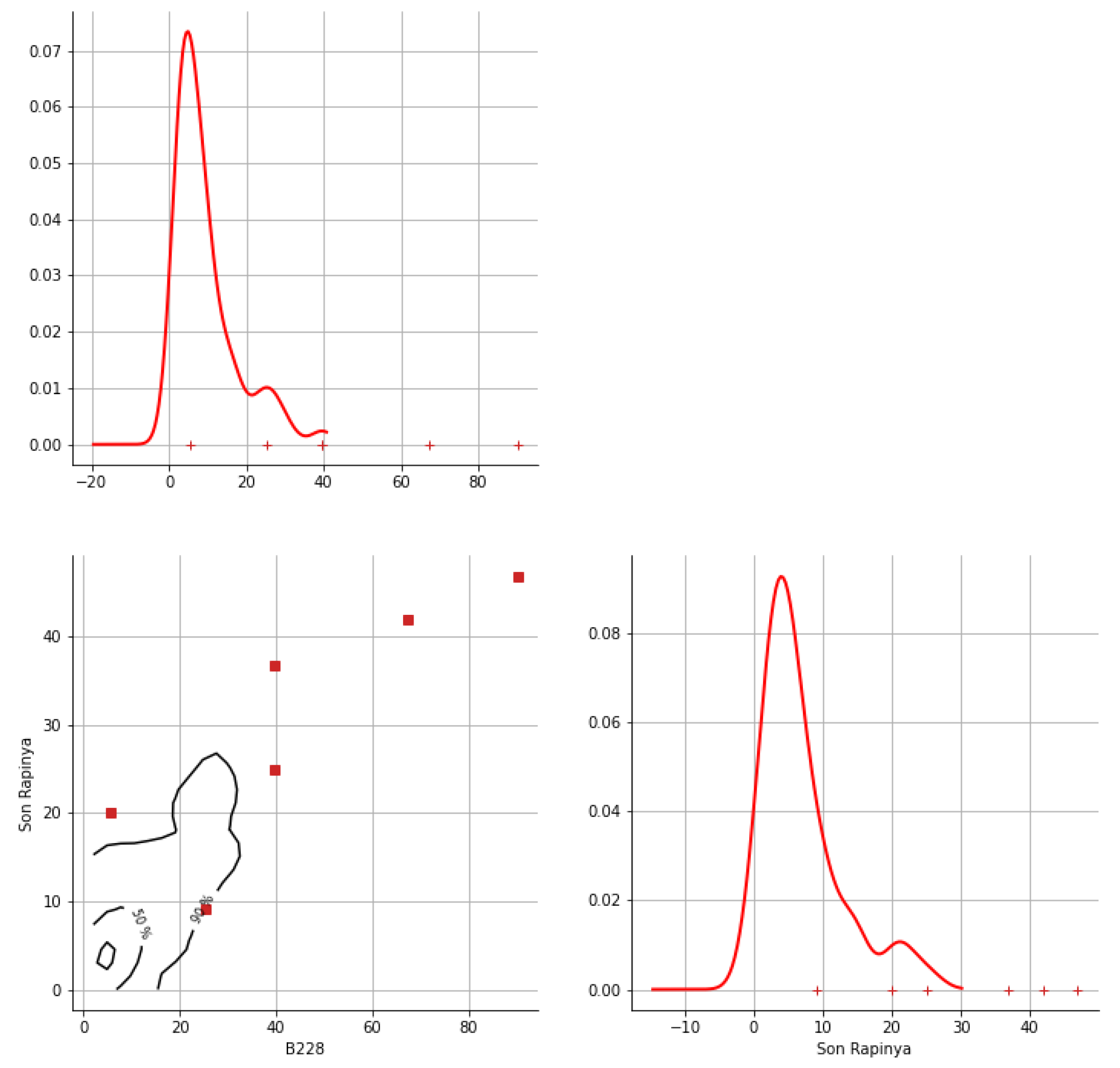
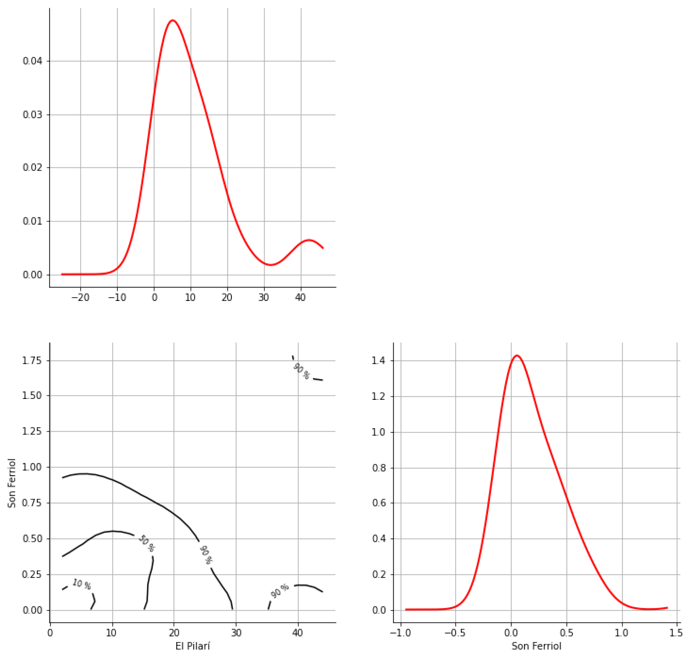
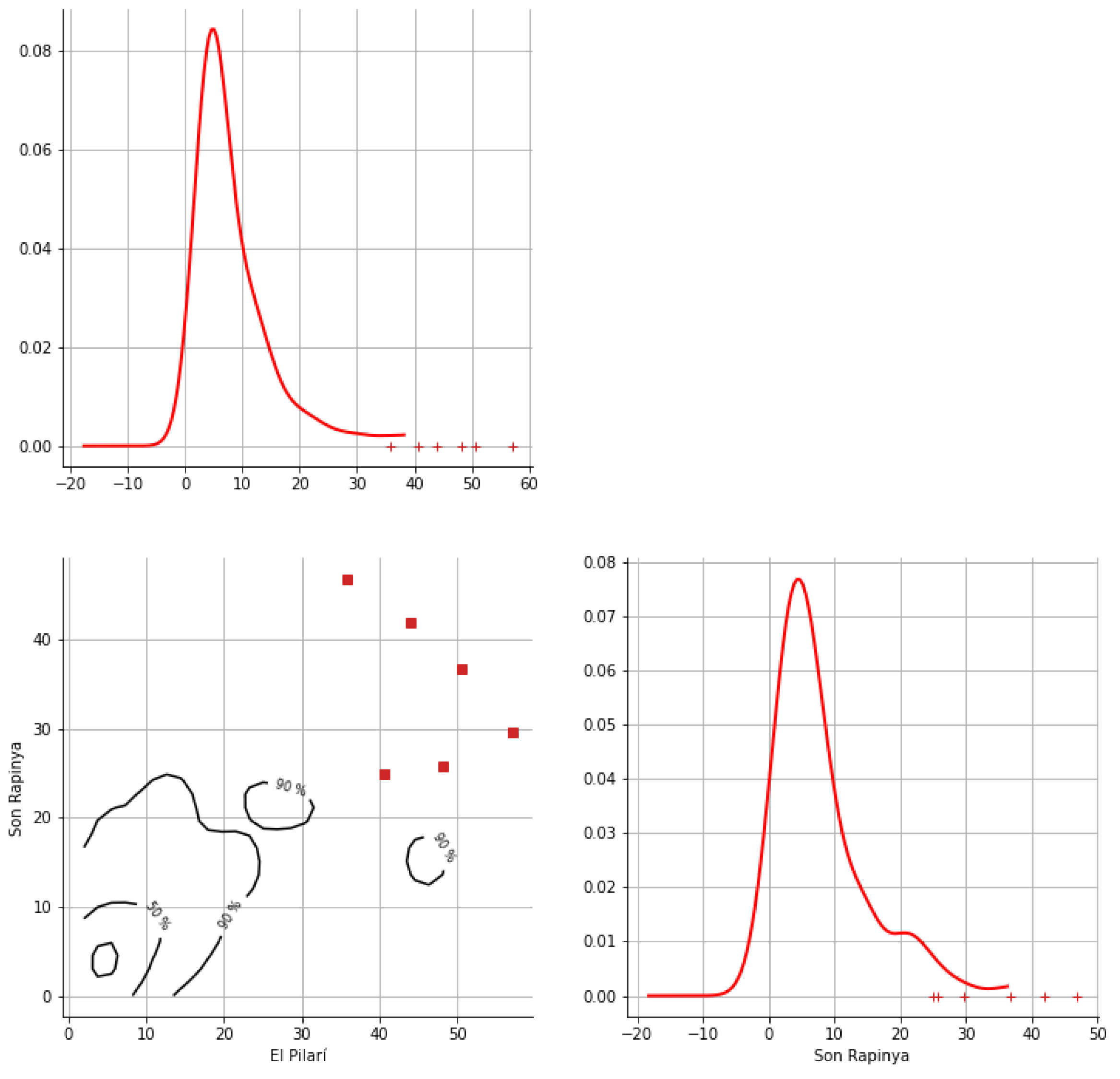
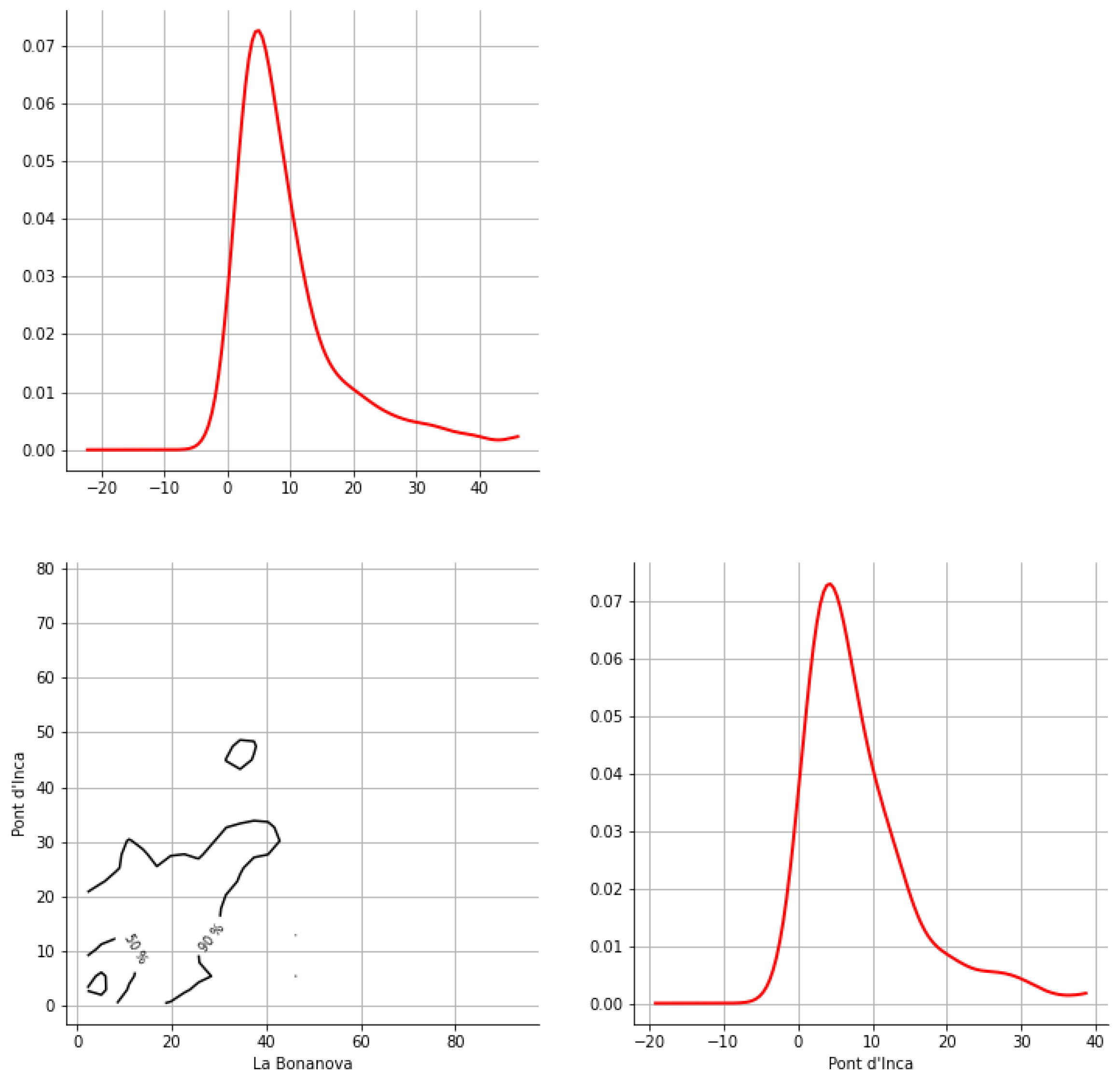
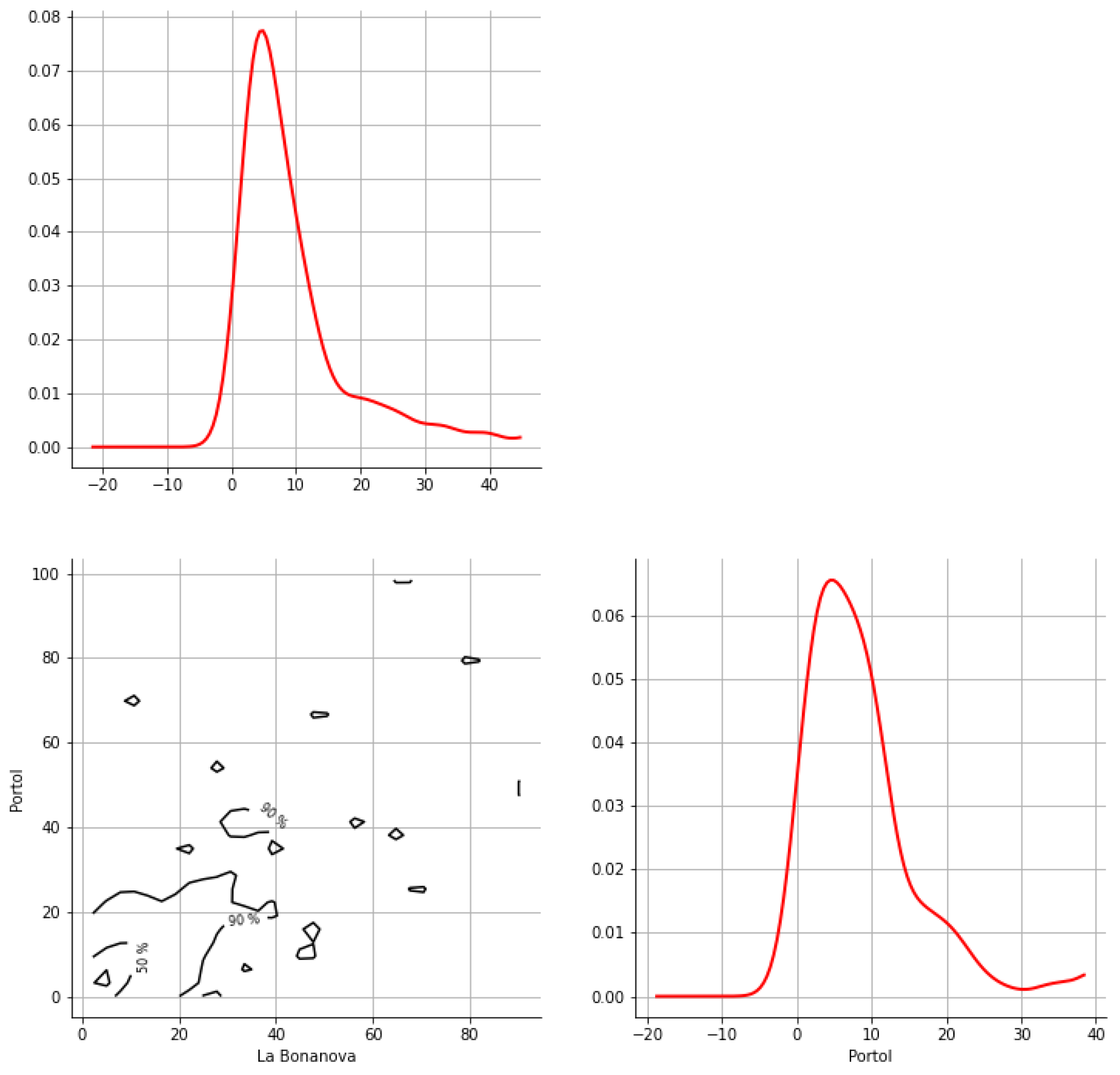
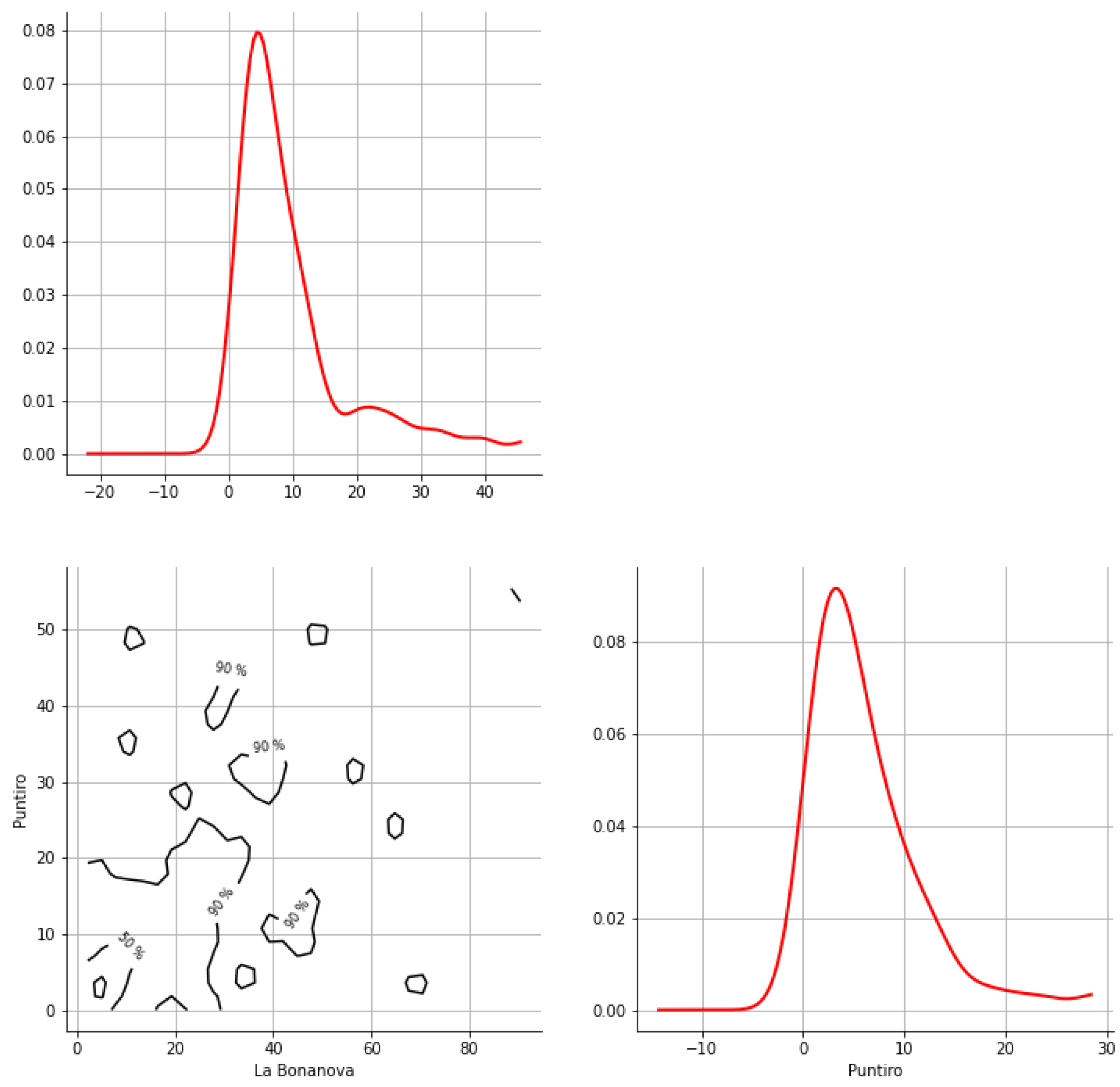
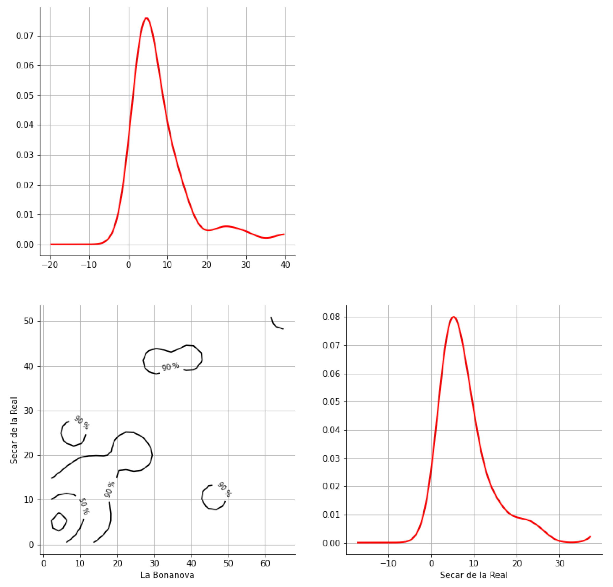
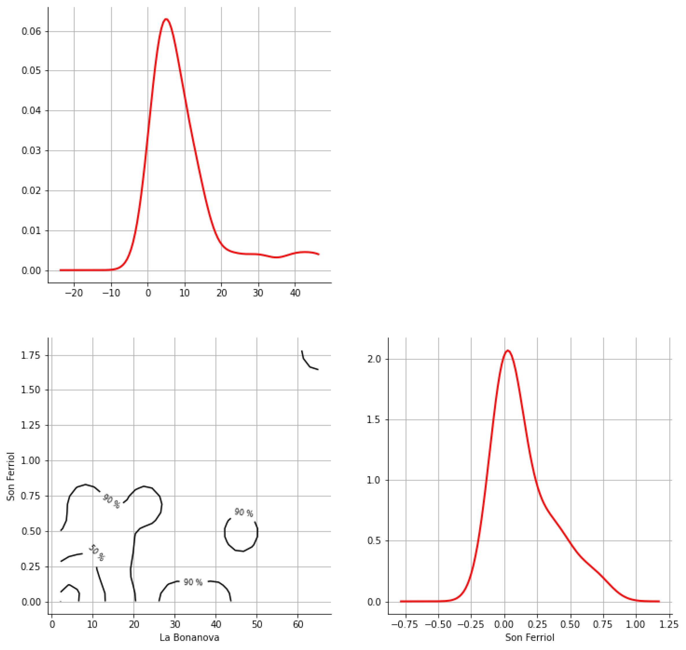
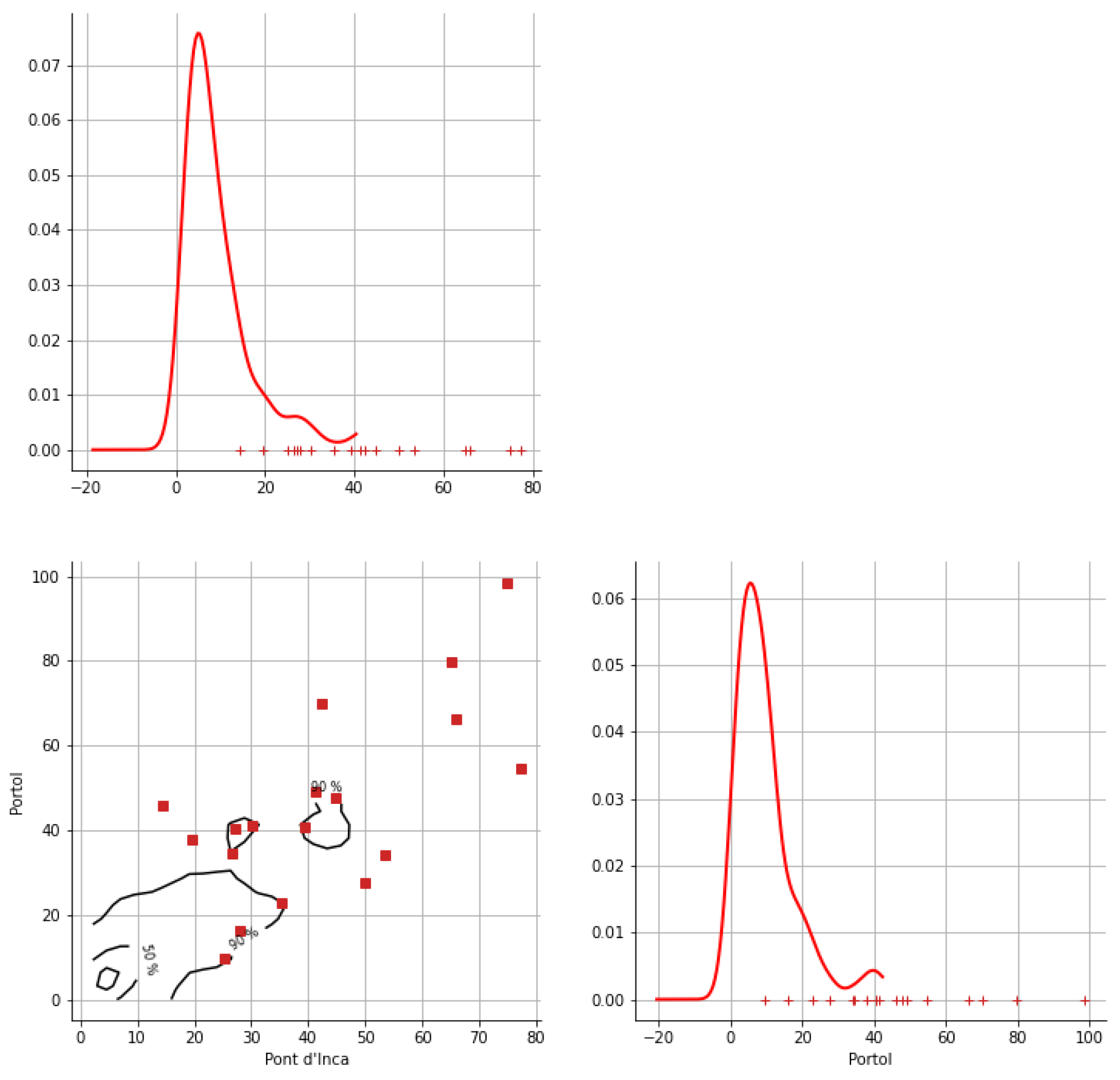
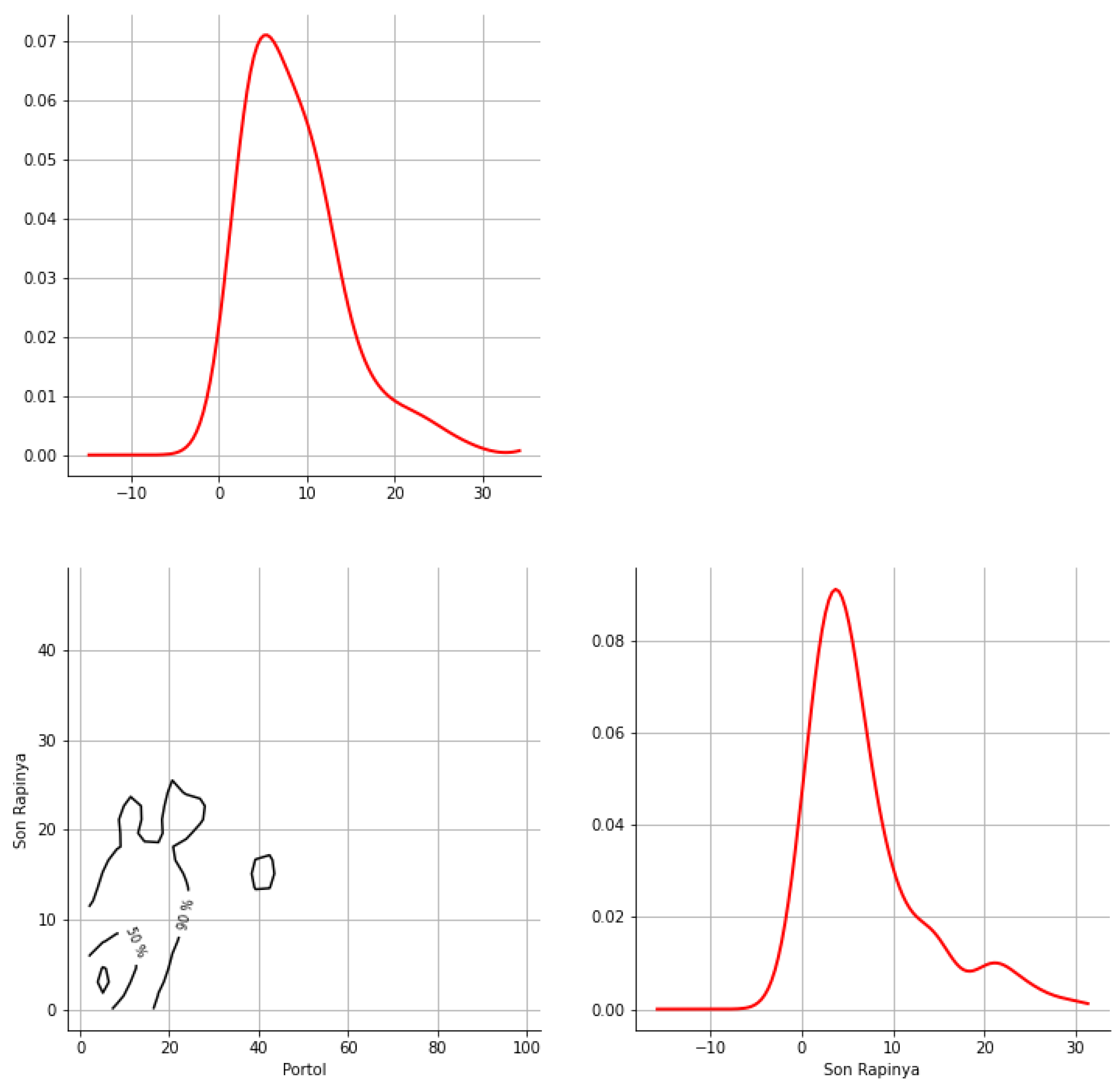
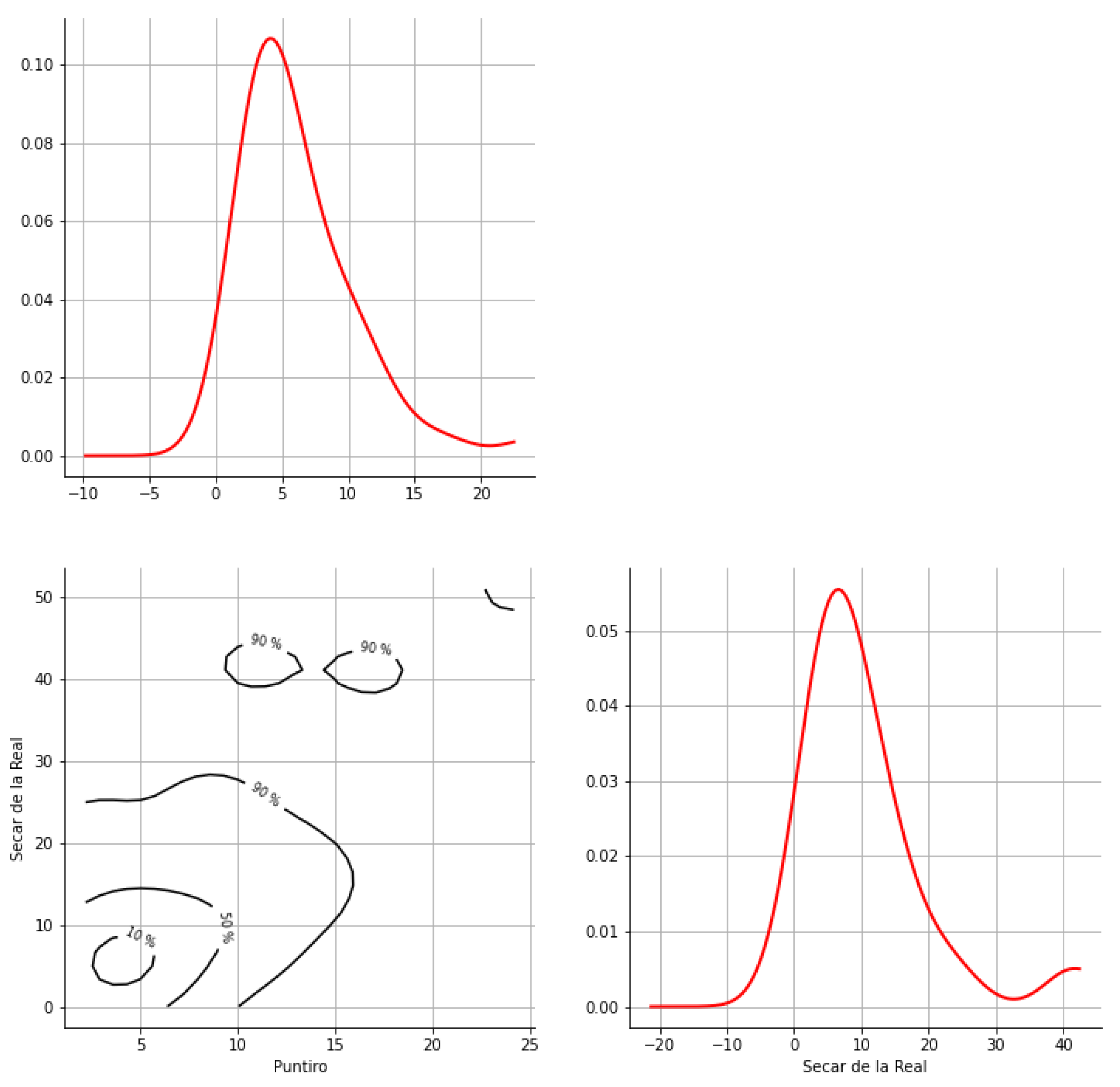
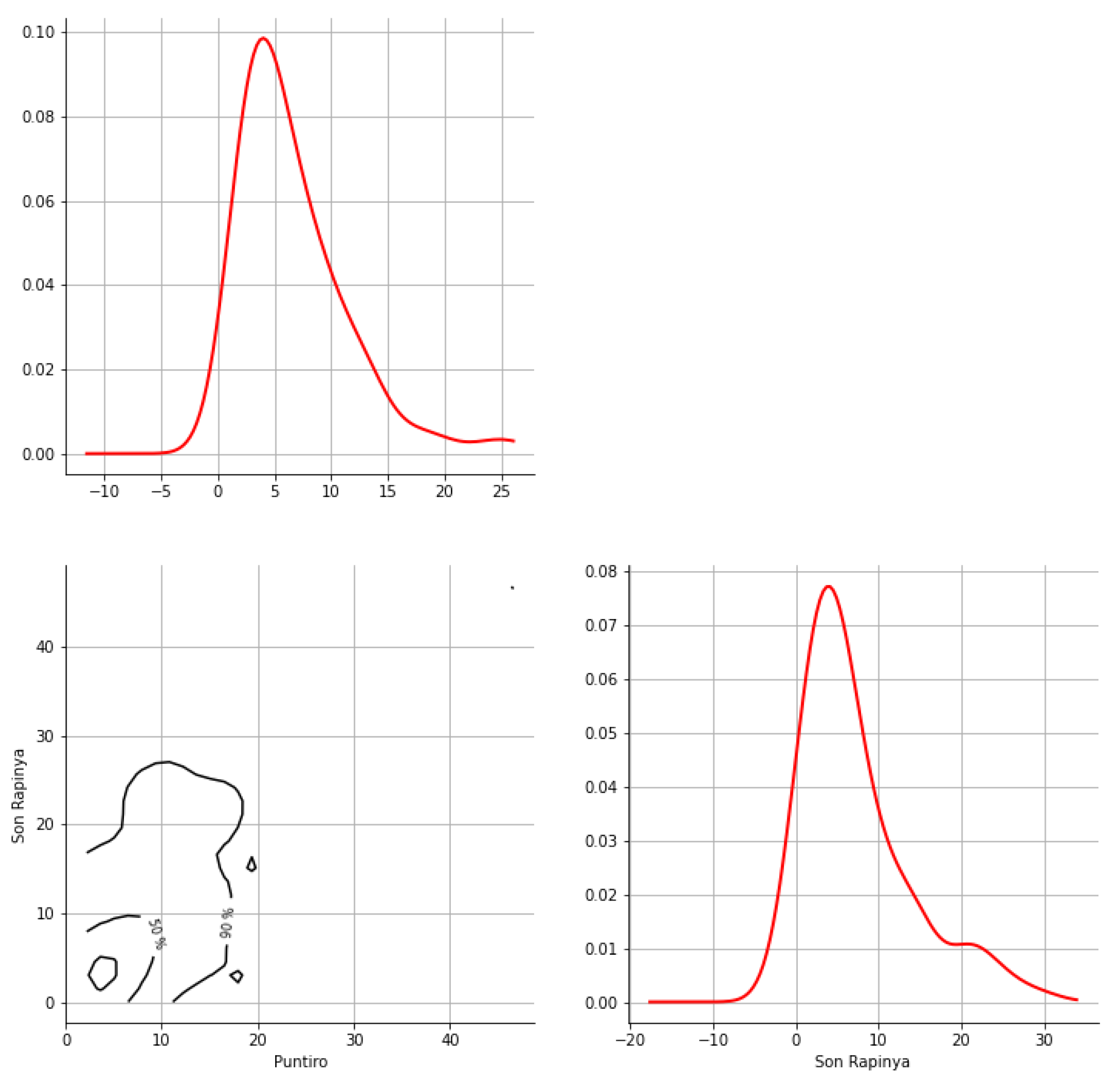
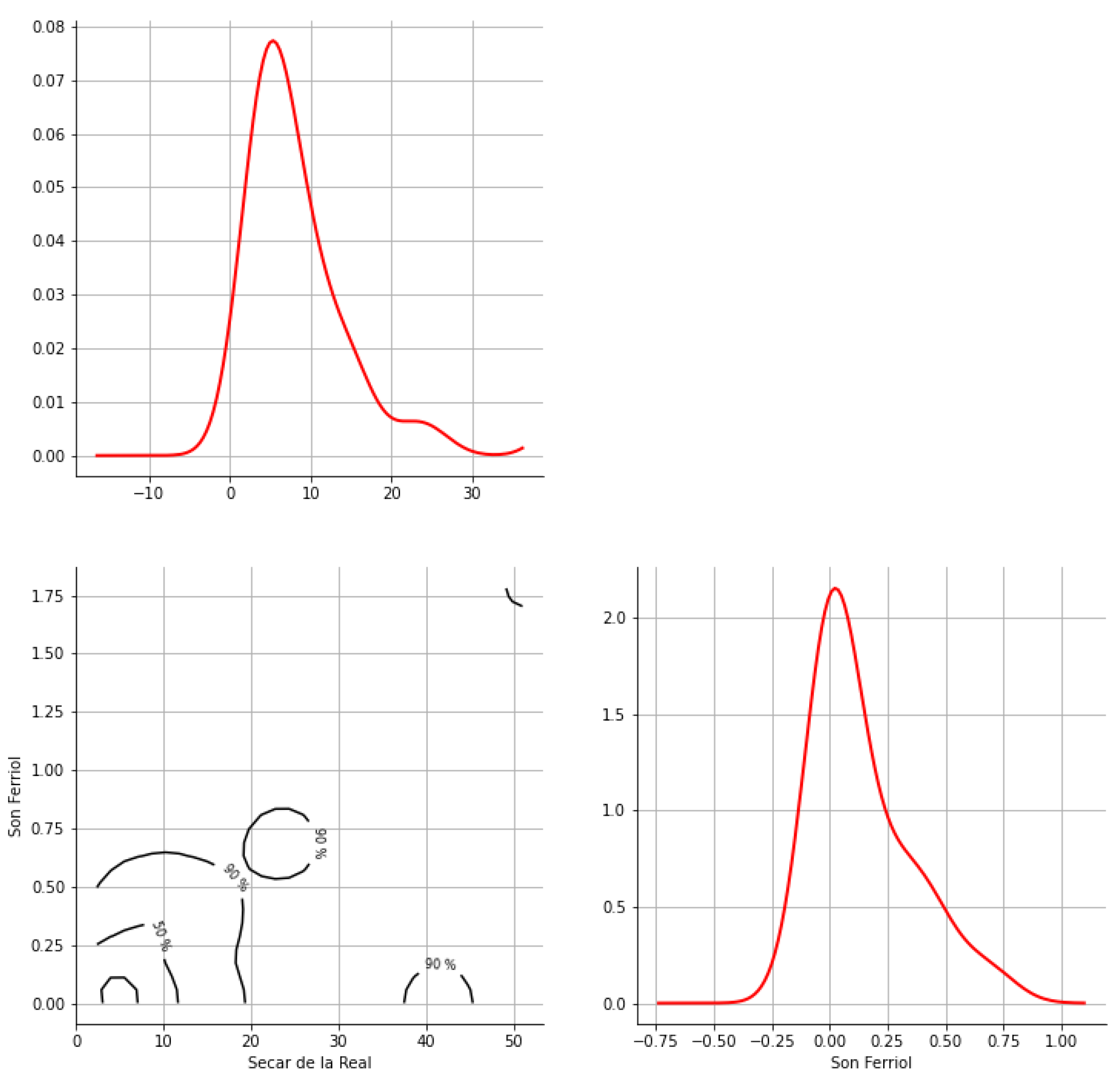
Appendix A. Bivariate HDR Boxplot Results


Appendix B. Detection of Occurrence of Rainfall Performance

| Combinations | POD | FAR | CSI | BS |
|---|---|---|---|---|
| El Pil·lari - La Bonanova - Pòrtol - Son Rapinya - Pont d’Inca - Puntiró - Secar de la Real | 0.94 | 0.18 | 0.79 | 1.15 |
| El Pil·lari - La Bonanova - Pòrtol - Son Rapinya - Pont d’Inca - Puntiró - B228 | 0.95 | 0.18 | 0.79 | 1.16 |
| El Pil·lari - La Bonanova - Pòrtol - Son Rapinya - Pont d’Inca - Puntiró - B236 | 0.94 | 0.18 | 0.78 | 1.15 |
| El Pil·lari - La Bonanova - Pòrtol - Son Rapinya - Pont d’Inca - Puntiró - B278 | 0.95 | 0.19 | 0.78 | 1.16 |
| El Pil·lari - La Bonanova - Pòrtol - Son Rapinya - Pont d’Inca - Secar de la Real - B228 | 0.92 | 0.17 | 0.78 | 1.12 |
| El Pil·lari - La Bonanova - Pòrtol - Son Rapinya - Pont d’Inca - Secar de la Real - B236 | 0.92 | 0.18 | 0.77 | 1.13 |
| El Pil·lari - La Bonanova - Pòrtol - Son Rapinya - Pont d’Inca - Secar de la Real - B278 | 0.93 | 0.19 | 0.76 | 1.15 |
| El Pil·lari - La Bonanova - Pòrtol - Son Rapinya - Pont d’Inca - B228 - B236 | 0.93 | 0.19 | 0.77 | 1.14 |
| El Pil·lari - La Bonanova - Pòrtol - Son Rapinya - Pont d’Inca - B228 - B278 | 0.93 | 0.18 | 0.77 | 1.14 |
| El Pil·lari - La Bonanova - Pòrtol - Son Rapinya - Pont d’Inca - B236 - B278 | 0.92 | 0.21 | 0.74 | 1.16 |
| El Pil·lari - La Bonanova - Pòrtol - Son Rapinya - Puntiró - Secar de la Real - B228 | 0.94 | 0.15 | 0.81 | 1.10 |
| El Pil·lari - La Bonanova - Pòrtol - Son Rapinya - Puntiró - Secar de la Real - B236 | 0.94 | 0.17 | 0.79 | 1.13 |
| El Pil·lari - La Bonanova - Pòrtol - Son Rapinya - Puntiró - Secar de la Real - B278 | 0.95 | 0.17 | 0.79 | 1.15 |
| El Pil·lari - La Bonanova - Pòrtol - Son Rapinya - Puntiró - B228 - B236 | 0.95 | 0.17 | 0.80 | 1.14 |
| El Pil·lari - La Bonanova - Pòrtol - Son Rapinya - Puntiró - B228 - B278 | 0.95 | 0.17 | 0.80 | 1.14 |
| El Pil·lari - La Bonanova - Pòrtol - Son Rapinya - Puntiró - B236 - B278 | 0.94 | 0.19 | 0.77 | 1.17 |
| El Pil·lari - La Bonanova - Pòrtol - Son Rapinya - Secar de la Real - B228 - B236 | 0.93 | 0.15 | 0.80 | 1.10 |
| El Pil·lari - La Bonanova - Pòrtol - Son Rapinya - Secar de la Real - B228 - B278 | 0.93 | 0.17 | 0.79 | 1.12 |
| El Pil·lari - La Bonanova - Pòrtol - Son Rapinya - Secar de la Real - B236 - B278 | 0.93 | 0.19 | 0.77 | 1.14 |
| El Pil·lari - La Bonanova - Pòrtol - Son Rapinya - B228 - B236 - B278 | 0.93 | 0.19 | 0.77 | 1.14 |
| El Pil·lari - La Bonanova - Pòrtol - Pont d’Inca - Puntiró - Secar de la Real - B228 | 0.95 | 0.17 | 0.80 | 1.14 |
| El Pil·lari - La Bonanova - Pòrtol - Pont d’Inca - Puntiró - Secar de la Real - B236 | 0.95 | 0.19 | 0.77 | 1.17 |
| El Pil·lari - La Bonanova - Pòrtol - Pont d’Inca - Puntiró - Secar de la Real - B278 | 0.95 | 0.20 | 0.77 | 1.18 |
| El Pil·lari - La Bonanova - Pòrtol - Pont d’Inca - Puntiró - B228 - B236 | 0.94 | 0.17 | 0.79 | 1.14 |
| El Pil·lari - La Bonanova - Pòrtol - Pont d’Inca - Puntiró - B228 - B278 | 0.95 | 0.17 | 0.79 | 1.14 |
| El Pil·lari - La Bonanova - Pòrtol - Pont d’Inca - Puntiró - B236 - B278 | 0.93 | 0.21 | 0.74 | 1.18 |
| El Pil·lari - La Bonanova - Pòrtol - Pont d’Inca - Secar de la Real - B228 - B236 | 0.93 | 0.17 | 0.78 | 1.12 |
| El Pil·lari - La Bonanova - Pòrtol - Pont d’Inca - Secar de la Real - B228 - B278 | 0.93 | 0.19 | 0.77 | 1.14 |
| El Pil·lari - La Bonanova - Pòrtol - Pont d’Inca - Secar de la Real - B236 - B278 | 0.92 | 0.21 | 0.74 | 1.17 |
| El Pil·lari - La Bonanova - Pòrtol - Pont d’Inca - B228 - B236 - B278 | 0.92 | 0.20 | 0.75 | 1.15 |
| El Pil·lari - La Bonanova - Pòrtol - Puntiró - Secar de la Real - B228 - B236 | 0.95 | 0.15 | 0.81 | 1.13 |
| El Pil·lari - La Bonanova - Pòrtol - Puntiró - Secar de la Real - B228 - B278 | 0.95 | 0.16 | 0.80 | 1.13 |
| El Pil·lari - La Bonanova - Pòrtol - Puntiró - Secar de la Real - B236 - B278 | 0.93 | 0.19 | 0.76 | 1.15 |
| El Pil·lari - La Bonanova - Pòrtol - Puntiró - B228 - B236 - B278 | 0.94 | 0.18 | 0.78 | 1.15 |
| El Pil·lari - La Bonanova - Pòrtol - Secar de la Real - B228 - B236 - B278 | 0.94 | 0.17 | 0.79 | 1.14 |
| El Pil·lari - La Bonanova - Son Rapinya - Pont d’Inca - Puntiró - Secar de la Real - B228 | 0.93 | 0.16 | 0.79 | 1.11 |
| El Pil·lari - La Bonanova - Son Rapinya - Pont d’Inca - Puntiró - Secar de la Real - B236 | 0.93 | 0.18 | 0.77 | 1.13 |
| El Pil·lari - La Bonanova - Son Rapinya - Pont d’Inca - Puntiró - Secar de la Real - B278 | 0.93 | 0.19 | 0.77 | 1.14 |
| El Pil·lari - La Bonanova - Son Rapinya - Pont d’Inca - Puntiró - B228 - B236 | 0.93 | 0.19 | 0.76 | 1.15 |
| El Pil·lari - La Bonanova - Son Rapinya - Pont d’Inca - Puntiró - B228 - B278 | 0.93 | 0.18 | 0.77 | 1.13 |
| El Pil·lari - La Bonanova - Son Rapinya - Pont d’Inca - Puntiró - B236 - B278 | 0.92 | 0.20 | 0.74 | 1.16 |
| El Pil·lari - La Bonanova - Son Rapinya - Pont d’Inca - Secar de la Real - B228 - B236 | 0.94 | 0.16 | 0.80 | 1.11 |
| El Pil·lari - La Bonanova - Son Rapinya - Pont d’Inca - Secar de la Real - B228 - B278 | 0.94 | 0.17 | 0.79 | 1.13 |
| El Pil·lari - La Bonanova - Son Rapinya - Pont d’Inca - Secar de la Real - B236 - B278 | 0.93 | 0.19 | 0.76 | 1.15 |
| El Pil·lari - La Bonanova - Son Rapinya - Pont d’Inca - B228 - B236 - B278 | 0.93 | 0.19 | 0.77 | 1.15 |
| El Pil·lari - La Bonanova - Son Rapinya - Puntiró - Secar de la Real - B228 - B236 | 0.93 | 0.15 | 0.80 | 1.10 |
| El Pil·lari - La Bonanova - Son Rapinya - Puntiró - Secar de la Real - B228 - B278 | 0.93 | 0.16 | 0.79 | 1.11 |
| El Pil·lari - La Bonanova - Son Rapinya - Puntiró - Secar de la Real - B236 - B278 | 0.92 | 0.19 | 0.76 | 1.13 |
| El Pil·lari - La Bonanova - Son Rapinya - Puntiró - B228 - B236 - B278 | 0.93 | 0.18 | 0.77 | 1.13 |
| El Pil·lari - La Bonanova - Son Rapinya - Secar de la Real - B228 - B236 - B278 | 0.93 | 0.16 | 0.79 | 1.12 |
| El Pil·lari - La Bonanova - Pont d’Inca - Puntiró - Secar de la Real - B228 - B236 | 0.93 | 0.17 | 0.78 | 1.13 |
| El Pil·lari - La Bonanova - Pont d’Inca - Puntiró - Secar de la Real - B228 - B278 | 0.93 | 0.18 | 0.77 | 1.12 |
| El Pil·lari - La Bonanova - Pont d’Inca - Puntiró - Secar de la Real - B236 - B278 | 0.92 | 0.21 | 0.74 | 1.16 |
| El Pil·lari - La Bonanova - Pont d’Inca - Puntiró - B228 - B236 - B278 | 0.93 | 0.20 | 0.76 | 1.16 |
| El Pil·lari - La Bonanova - Pont d’Inca - Secar de la Real - B228 - B236 - B278 | 0.94 | 0.17 | 0.78 | 1.13 |
| El Pil·lari - La Bonanova - Puntiró - Secar de la Real - B228 - B236 - B278 | 0.94 | 0.17 | 0.79 | 1.12 |
| El Pil·lari - Pòrtol - Son Rapinya - Pont d’Inca - Puntiró - Secar de la Real - B228 | 0.94 | 0.17 | 0.79 | 1.13 |
| El Pil·lari - Pòrtol - Son Rapinya - Pont d’Inca - Puntiró - Secar de la Real - B236 | 0.95 | 0.18 | 0.78 | 1.16 |
| El Pil·lari - Pòrtol - Son Rapinya - Pont d’Inca - Puntiró - Secar de la Real - B278 | 0.95 | 0.19 | 0.78 | 1.18 |
| El Pil·lari - Pòrtol - Son Rapinya - Pont d’Inca - Puntiró - B228 - B236 | 0.93 | 0.18 | 0.77 | 1.14 |
| El Pil·lari - Pòrtol - Son Rapinya - Pont d’Inca - Puntiró - B228 - B278 | 0.94 | 0.18 | 0.78 | 1.15 |
| El Pil·lari - Pòrtol - Son Rapinya - Pont d’Inca - Puntiró - B236 - B278 | 0.94 | 0.20 | 0.76 | 1.17 |
| El Pil·lari - Pòrtol - Son Rapinya - Pont d’Inca - Secar de la Real - B228 - B236 | 0.92 | 0.18 | 0.76 | 1.12 |
| El Pil·lari - Pòrtol - Son Rapinya - Pont d’Inca - Secar de la Real - B228 - B278 | 0.92 | 0.19 | 0.76 | 1.14 |
| El Pil·lari - Pòrtol - Son Rapinya - Pont d’Inca - Secar de la Real - B236 - B278 | 0.93 | 0.21 | 0.75 | 1.17 |
| El Pil·lari - Pòrtol - Son Rapinya - Pont d’Inca - B228 - B236 - B278 | 0.91 | 0.20 | 0.74 | 1.14 |
| El Pil·lari - Pòrtol - Son Rapinya - Puntiró - Secar de la Real - B228 - B236 | 0.93 | 0.16 | 0.79 | 1.11 |
| El Pil·lari - Pòrtol - Son Rapinya - Puntiró - Secar de la Real - B228 - B278 | 0.95 | 0.17 | 0.79 | 1.13 |
| El Pil·lari - Pòrtol - Son Rapinya - Puntiró - Secar de la Real - B236 - B278 | 0.94 | 0.19 | 0.77 | 1.15 |
| El Pil·lari - Pòrtol - Son Rapinya - Puntiró - B228 - B236 - B278 | 0.93 | 0.19 | 0.77 | 1.15 |
| El Pil·lari - Pòrtol - Son Rapinya - Secar de la Real - B228 - B236 - B278 | 0.93 | 0.19 | 0.76 | 1.14 |
| El Pil·lari - Pòrtol - Pont d’Inca - Puntiró - Secar de la Real - B228 - B236 | 0.94 | 0.19 | 0.77 | 1.16 |
| El Pil·lari - Pòrtol - Pont d’Inca - Puntiró - Secar de la Real - B228 - B278 | 0.95 | 0.19 | 0.78 | 1.16 |
| El Pil·lari - Pòrtol - Pont d’Inca - Puntiró - Secar de la Real - B236 - B278 | 0.93 | 0.20 | 0.76 | 1.16 |
| El Pil·lari - Pòrtol - Pont d’Inca - Puntiró - B228 - B236 - B278 | 0.92 | 0.20 | 0.75 | 1.16 |
| El Pil·lari - Pòrtol - Pont d’Inca - Secar de la Real - B228 - B236 - B278 | 0.92 | 0.21 | 0.74 | 1.16 |
| El Pil·lari - Pòrtol - Puntiró - Secar de la Real - B228 - B236 - B278 | 0.94 | 0.18 | 0.77 | 1.14 |
| El Pil·lari - Son Rapinya - Pont d’Inca - Puntiró - Secar de la Real - B228 - B236 | 0.92 | 0.18 | 0.76 | 1.13 |
| El Pil·lari - Son Rapinya - Pont d’Inca - Puntiró - Secar de la Real - B228 - B278 | 0.92 | 0.18 | 0.77 | 1.12 |
| El Pil·lari - Son Rapinya - Pont d’Inca - Puntiró - Secar de la Real - B236 - B278 | 0.93 | 0.20 | 0.75 | 1.16 |
| El Pil·lari - Son Rapinya - Pont d’Inca - Puntiró - B228 - B236 - B278 | 0.91 | 0.20 | 0.74 | 1.14 |
| El Pil·lari - Son Rapinya - Pont d’Inca - Secar de la Real - B228 - B236 - B278 | 0.92 | 0.19 | 0.76 | 1.14 |
| El Pil·lari - Son Rapinya - Puntiró - Secar de la Real - B228 - B236 - B278 | 0.92 | 0.18 | 0.76 | 1.12 |
| El Pil·lari - Pont d’Inca - Puntiró - Secar de la Real - B228 - B236 - B278 | 0.92 | 0.20 | 0.75 | 1.15 |
| La Bonanova - Pòrtol - Son Rapinya - Pont d’Inca - Puntiró - Secar de la Real - B228 | 0.95 | 0.14 | 0.83 | 1.11 |
| La Bonanova - Pòrtol - Son Rapinya - Pont d’Inca - Puntiró - Secar de la Real - B236 | 0.95 | 0.15 | 0.81 | 1.12 |
| La Bonanova - Pòrtol - Son Rapinya - Pont d’Inca - Puntiró - Secar de la Real - B278 | 0.95 | 0.17 | 0.80 | 1.14 |
| La Bonanova - Pòrtol - Son Rapinya - Pont d’Inca - Puntiró - B228 - B236 | 0.96 | 0.15 | 0.81 | 1.13 |
| La Bonanova - Pòrtol - Son Rapinya - Pont d’Inca - Puntiró - B228 - B278 | 0.95 | 0.15 | 0.81 | 1.13 |
| La Bonanova - Pòrtol - Son Rapinya - Pont d’Inca - Puntiró - B236 - B278 | 0.94 | 0.17 | 0.79 | 1.14 |
| La Bonanova - Pòrtol - Son Rapinya - Pont d’Inca - Secar de la Real - B228 - B236 | 0.95 | 0.15 | 0.81 | 1.11 |
| La Bonanova - Pòrtol - Son Rapinya - Pont d’Inca - Secar de la Real - B228 - B278 | 0.93 | 0.16 | 0.79 | 1.10 |
| La Bonanova - Pòrtol - Son Rapinya - Pont d’Inca - Secar de la Real - B236 - B278 | 0.94 | 0.17 | 0.79 | 1.14 |
| La Bonanova - Pòrtol - Son Rapinya - Pont d’Inca - B228 - B236 - B278 | 0.95 | 0.17 | 0.79 | 1.14 |
| La Bonanova - Pòrtol - Son Rapinya - Puntiró - Secar de la Real - B228 - B236 | 0.95 | 0.12 | 0.84 | 1.08 |
| La Bonanova - Pòrtol - Son Rapinya - Puntiró - Secar de la Real - B228 - B278 | 0.95 | 0.13 | 0.83 | 1.09 |
| La Bonanova - Pòrtol - Son Rapinya - Puntiró - Secar de la Real - B236 - B278 | 0.95 | 0.15 | 0.81 | 1.11 |
| La Bonanova - Pòrtol - Son Rapinya - Puntiró - B228 - B236 - B278 | 0.95 | 0.15 | 0.82 | 1.11 |
| La Bonanova - Pòrtol - Son Rapinya - Secar de la Real - B228 - B236 - B278 | 0.94 | 0.15 | 0.81 | 1.11 |
| La Bonanova - Pòrtol - Pont d’Inca - Puntiró - Secar de la Real - B228 - B236 | 0.96 | 0.14 | 0.83 | 1.11 |
| La Bonanova - Pòrtol - Pont d’Inca - Puntiró - Secar de la Real - B228 - B278 | 0.95 | 0.15 | 0.81 | 1.12 |
| La Bonanova - Pòrtol - Pont d’Inca - Puntiró - Secar de la Real - B236 - B278 | 0.95 | 0.18 | 0.79 | 1.15 |
| La Bonanova - Pòrtol - Pont d’Inca - Puntiró - B228 - B236 - B278 | 0.95 | 0.16 | 0.80 | 1.14 |
| La Bonanova - Pòrtol - Pont d’Inca - Secar de la Real - B228 - B236 - B278 | 0.95 | 0.17 | 0.80 | 1.14 |
| La Bonanova - Pòrtol - Puntiró - Secar de la Real - B228 - B236 - B278 | 0.96 | 0.14 | 0.83 | 1.11 |
| La Bonanova - Son Rapinya - Pont d’Inca - Puntiró - Secar de la Real - B228 - B236 | 0.94 | 0.14 | 0.81 | 1.09 |
| La Bonanova - Son Rapinya - Pont d’Inca - Puntiró - Secar de la Real - B228 - B278 | 0.93 | 0.15 | 0.80 | 1.10 |
| La Bonanova - Son Rapinya - Pont d’Inca - Puntiró - Secar de la Real - B236 - B278 | 0.94 | 0.17 | 0.79 | 1.13 |
| La Bonanova - Son Rapinya - Pont d’Inca - Puntiró - B228 - B236 - B278 | 0.94 | 0.17 | 0.78 | 1.13 |
| La Bonanova - Son Rapinya - Pont d’Inca - Secar de la Real - B228 - B236 - B278 | 0.95 | 0.15 | 0.81 | 1.11 |
| La Bonanova - Son Rapinya - Puntiró - Secar de la Real - B228 - B236 - B278 | 0.93 | 0.15 | 0.81 | 1.09 |
| La Bonanova - Pont d’Inca - Puntiró - Secar de la Real - B228 - B236 - B278 | 0.94 | 0.16 | 0.79 | 1.12 |
| Pòrtol - Son Rapinya - Pont d’Inca - Puntiró - Secar de la Real - B228 - B236 | 0.94 | 0.15 | 0.81 | 1.11 |
| Pòrtol - Son Rapinya - Pont d’Inca - Puntiró - Secar de la Real - B228 - B278 | 0.94 | 0.16 | 0.80 | 1.12 |
| Pòrtol - Son Rapinya - Pont d’Inca - Puntiró - Secar de la Real - B236 - B278 | 0.95 | 0.18 | 0.79 | 1.15 |
| Pòrtol - Son Rapinya - Pont d’Inca - Puntiró - B228 - B236 - B278 | 0.94 | 0.17 | 0.79 | 1.13 |
| Pòrtol - Son Rapinya - Pont d’Inca - Secar de la Real - B228 - B236 - B278 | 0.93 | 0.18 | 0.78 | 1.13 |
| Pòrtol - Son Rapinya - Puntiró - Secar de la Real - B228 - B236 - B278 | 0.94 | 0.15 | 0.81 | 1.11 |
| Pòrtol - Pont d’Inca - Puntiró - Secar de la Real - B228 - B236 - B278 | 0.94 | 0.17 | 0.79 | 1.14 |
| Son Rapinya - Pont d’Inca - Puntiró - Secar de la Real - B228 - B236 - B278 | 0.93 | 0.17 | 0.78 | 1.12 |
Appendix C. Accuracy of Rainfall Performance
| Combinations | <1 mm | >40 mm | |||
|---|---|---|---|---|---|
| El Pil·lari - La Bonanova - Pòrtol - Son Rapinya - Pont d’Inca - Puntiró - Secar de la Real | 0.81 | 0.44 | 0.56 | 0.28 | 0.50 |
| El Pil·lari - La Bonanova - Pòrtol - Son Rapinya - Pont d’Inca - Puntiró - B228 | 0.83 | 0.49 | 0.60 | 0.39 | 0.62 |
| El Pil·lari - La Bonanova - Pòrtol - Son Rapinya - Pont d’Inca - Puntiró - B236 | 0.77 | 0.41 | 0.54 | 0.41 | 0.62 |
| El Pil·lari - La Bonanova - Pòrtol - Son Rapinya - Pont d’Inca - Puntiró - B278 | 0.82 | 0.45 | 0.58 | 0.36 | 0.62 |
| El Pil·lari - La Bonanova - Pòrtol - Son Rapinya - Pont d’Inca - Secar de la Real - B228 | 0.82 | 0.47 | 0.59 | 0.38 | 0.50 |
| El Pil·lari - La Bonanova - Pòrtol - Son Rapinya - Pont d’Inca - Secar de la Real - B236 | 0.78 | 0.40 | 0.53 | 0.31 | 0.50 |
| El Pil·lari - La Bonanova - Pòrtol - Son Rapinya - Pont d’Inca - Secar de la Real - B278 | 0.79 | 0.42 | 0.55 | 0.35 | 0.55 |
| El Pil·lari - La Bonanova - Pòrtol - Son Rapinya - Pont d’Inca - B228 - B236 | 0.80 | 0.44 | 0.57 | 0.50 | 0.67 |
| El Pil·lari - La Bonanova - Pòrtol - Son Rapinya - Pont d’Inca - B228 - B278 | 0.83 | 0.50 | 0.62 | 0.53 | 0.67 |
| El Pil·lari - La Bonanova - Pòrtol - Son Rapinya - Pont d’Inca - B236 - B278 | 0.77 | 0.41 | 0.56 | 0.48 | 0.67 |
| El Pil·lari - La Bonanova - Pòrtol - Son Rapinya - Puntiró - Secar de la Real - B228 | 0.83 | 0.47 | 0.58 | 0.29 | 0.45 |
| El Pil·lari - La Bonanova - Pòrtol - Son Rapinya - Puntiró - Secar de la Real - B236 | 0.77 | 0.41 | 0.53 | 0.30 | 0.45 |
| El Pil·lari - La Bonanova - Pòrtol - Son Rapinya - Puntiró - Secar de la Real - B278 | 0.80 | 0.44 | 0.55 | 0.27 | 0.50 |
| El Pil·lari - La Bonanova - Pòrtol - Son Rapinya - Puntiró - B228 - B236 | 0.79 | 0.44 | 0.56 | 0.42 | 0.62 |
| El Pil·lari - La Bonanova - Pòrtol - Son Rapinya - Puntiró - B228 - B278 | 0.82 | 0.48 | 0.59 | 0.42 | 0.62 |
| El Pil·lari - La Bonanova - Pòrtol - Son Rapinya - Puntiró - B236 - B278 | 0.75 | 0.41 | 0.55 | 0.40 | 0.62 |
| El Pil·lari - La Bonanova - Pòrtol - Son Rapinya - Secar de la Real - B228 - B236 | 0.79 | 0.44 | 0.58 | 0.38 | 0.50 |
| El Pil·lari - La Bonanova - Pòrtol - Son Rapinya - Secar de la Real - B228 - B278 | 0.80 | 0.45 | 0.58 | 0.42 | 0.55 |
| El Pil·lari - La Bonanova - Pòrtol - Son Rapinya - Secar de la Real - B236 - B278 | 0.76 | 0.41 | 0.53 | 0.38 | 0.55 |
| El Pil·lari - La Bonanova - Pòrtol - Son Rapinya - B228 - B236 - B278 | 0.78 | 0.43 | 0.57 | 0.52 | 0.67 |
| El Pil·lari - La Bonanova - Pòrtol - Pont d’Inca - Puntiró - Secar de la Real - B228 | 0.82 | 0.46 | 0.59 | 0.31 | 0.45 |
| El Pil·lari - La Bonanova - Pòrtol - Pont d’Inca - Puntiró - Secar de la Real - B236 | 0.76 | 0.37 | 0.55 | 0.33 | 0.50 |
| El Pil·lari - La Bonanova - Pòrtol - Pont d’Inca - Puntiró - Secar de la Real - B278 | 0.79 | 0.38 | 0.53 | 0.28 | 0.50 |
| El Pil·lari - La Bonanova - Pòrtol - Pont d’Inca - Puntiró - B228 - B236 | 0.78 | 0.43 | 0.57 | 0.47 | 0.56 |
| El Pil·lari - La Bonanova - Pòrtol - Pont d’Inca - Puntiró - B228 - B278 | 0.83 | 0.46 | 0.60 | 0.38 | 0.56 |
| El Pil·lari - La Bonanova - Pòrtol - Pont d’Inca - Puntiró - B236 - B278 | 0.75 | 0.37 | 0.53 | 0.48 | 0.62 |
| El Pil·lari - La Bonanova - Pòrtol - Pont d’Inca - Secar de la Real - B228 - B236 | 0.78 | 0.41 | 0.56 | 0.40 | 0.50 |
| El Pil·lari - La Bonanova - Pòrtol - Pont d’Inca - Secar de la Real - B228 - B278 | 0.79 | 0.41 | 0.56 | 0.36 | 0.50 |
| El Pil·lari - La Bonanova - Pòrtol - Pont d’Inca - Secar de la Real - B236 - B278 | 0.75 | 0.35 | 0.51 | 0.35 | 0.55 |
| El Pil·lari - La Bonanova - Pòrtol - Pont d’Inca - B228 - B236 - B278 | 0.78 | 0.41 | 0.56 | 0.48 | 0.60 |
| El Pil·lari - La Bonanova - Pòrtol - Puntiró - Secar de la Real - B228 - B236 | 0.77 | 0.41 | 0.55 | 0.38 | 0.45 |
| El Pil·lari - La Bonanova - Pòrtol - Puntiró - Secar de la Real - B228 - B278 | 0.80 | 0.44 | 0.56 | 0.29 | 0.45 |
| El Pil·lari - La Bonanova - Pòrtol - Puntiró - Secar de la Real - B236 - B278 | 0.74 | 0.38 | 0.52 | 0.34 | 0.50 |
| El Pil·lari - La Bonanova - Pòrtol - Puntiró - B228 - B236 - B278 | 0.77 | 0.41 | 0.55 | 0.41 | 0.56 |
| El Pil·lari - La Bonanova - Pòrtol - Secar de la Real - B228 - B236 - B278 | 0.77 | 0.41 | 0.56 | 0.38 | 0.50 |
| El Pil·lari - La Bonanova - Son Rapinya - Pont d’Inca - Puntiró - Secar de la Real - B228 | 0.84 | 0.50 | 0.59 | 0.34 | 0.50 |
| El Pil·lari - La Bonanova - Son Rapinya - Pont d’Inca - Puntiró - Secar de la Real - B236 | 0.77 | 0.41 | 0.52 | 0.27 | 0.50 |
| El Pil·lari - La Bonanova - Son Rapinya - Pont d’Inca - Puntiró - Secar de la Real - B278 | 0.80 | 0.46 | 0.56 | 0.33 | 0.55 |
| El Pil·lari - La Bonanova - Son Rapinya - Pont d’Inca - Puntiró - B228 - B236 | 0.79 | 0.45 | 0.56 | 0.47 | 0.67 |
| El Pil·lari - La Bonanova - Son Rapinya - Pont d’Inca - Puntiró - B228 - B278 | 0.83 | 0.51 | 0.61 | 0.50 | 0.67 |
| El Pil·lari - La Bonanova - Son Rapinya - Pont d’Inca - Puntiró - B236 - B278 | 0.76 | 0.43 | 0.54 | 0.46 | 0.67 |
| El Pil·lari - La Bonanova - Son Rapinya - Pont d’Inca - Secar de la Real - B228 - B236 | 0.81 | 0.49 | 0.59 | 0.39 | 0.58 |
| El Pil·lari - La Bonanova - Son Rapinya - Pont d’Inca - Secar de la Real - B228 - B278 | 0.84 | 0.50 | 0.61 | 0.42 | 0.64 |
| El Pil·lari - La Bonanova - Son Rapinya - Pont d’Inca - Secar de la Real - B236 - B278 | 0.78 | 0.44 | 0.54 | 0.39 | 0.64 |
| El Pil·lari - La Bonanova - Son Rapinya - Pont d’Inca - B228 - B236 - B278 | 0.81 | 0.47 | 0.58 | 0.55 | 0.78 |
| El Pil·lari - La Bonanova - Son Rapinya - Puntiró - Secar de la Real - B228 - B236 | 0.79 | 0.45 | 0.57 | 0.34 | 0.50 |
| El Pil·lari - La Bonanova - Son Rapinya - Puntiró - Secar de la Real - B228 - B278 | 0.81 | 0.49 | 0.60 | 0.39 | 0.55 |
| El Pil·lari - La Bonanova - Son Rapinya - Puntiró - Secar de la Real - B236 - B278 | 0.76 | 0.41 | 0.52 | 0.33 | 0.55 |
| El Pil·lari - La Bonanova - Son Rapinya - Puntiró - B228 - B236 - B278 | 0.77 | 0.45 | 0.57 | 0.48 | 0.67 |
| El Pil·lari - La Bonanova - Son Rapinya - Secar de la Real - B228 - B236 - B278 | 0.80 | 0.48 | 0.58 | 0.45 | 0.64 |
| El Pil·lari - La Bonanova - Pont d’Inca - Puntiró - Secar de la Real - B228 - B236 | 0.78 | 0.43 | 0.56 | 0.36 | 0.50 |
| El Pil·lari - La Bonanova - Pont d’Inca - Puntiró - Secar de la Real - B228 - B278 | 0.79 | 0.44 | 0.56 | 0.34 | 0.50 |
| El Pil·lari - La Bonanova - Pont d’Inca - Puntiró - Secar de la Real - B236 - B278 | 0.74 | 0.37 | 0.50 | 0.31 | 0.55 |
| El Pil·lari - La Bonanova - Pont d’Inca - Puntiró - B228 - B236 - B278 | 0.77 | 0.41 | 0.55 | 0.46 | 0.60 |
| El Pil·lari - La Bonanova - Pont d’Inca - Secar de la Real - B228 - B236 - B278 | 0.78 | 0.43 | 0.55 | 0.42 | 0.64 |
| El Pil·lari - La Bonanova - Puntiró - Secar de la Real - B228 - B236 - B278 | 0.77 | 0.42 | 0.55 | 0.35 | 0.50 |
| El Pil·lari - Pòrtol - Son Rapinya - Pont d’Inca - Puntiró - Secar de la Real - B228 | 0.81 | 0.43 | 0.57 | 0.29 | 0.56 |
| El Pil·lari - Pòrtol - Son Rapinya - Pont d’Inca - Puntiró - Secar de la Real - B236 | 0.76 | 0.38 | 0.54 | 0.36 | 0.44 |
| El Pil·lari - Pòrtol - Son Rapinya - Pont d’Inca - Puntiró - Secar de la Real - B278 | 0.81 | 0.43 | 0.57 | 0.29 | 0.44 |
| El Pil·lari - Pòrtol - Son Rapinya - Pont d’Inca - Puntiró - B228 - B236 | 0.78 | 0.40 | 0.55 | 0.50 | 0.71 |
| El Pil·lari - Pòrtol - Son Rapinya - Pont d’Inca - Puntiró - B228 - B278 | 0.82 | 0.44 | 0.58 | 0.40 | 0.71 |
| El Pil·lari - Pòrtol - Son Rapinya - Pont d’Inca - Puntiró - B236 - B278 | 0.77 | 0.40 | 0.56 | 0.52 | 0.33 |
| El Pil·lari - Pòrtol - Son Rapinya - Pont d’Inca - Secar de la Real - B228 - B236 | 0.78 | 0.40 | 0.55 | 0.36 | 0.55 |
| El Pil·lari - Pòrtol - Son Rapinya - Pont d’Inca - Secar de la Real - B228 - B278 | 0.79 | 0.41 | 0.57 | 0.39 | 0.60 |
| El Pil·lari - Pòrtol - Son Rapinya - Pont d’Inca - Secar de la Real - B236 - B278 | 0.77 | 0.38 | 0.54 | 0.38 | 0.60 |
| El Pil·lari - Pòrtol - Son Rapinya - Pont d’Inca - B228 - B236 - B278 | 0.77 | 0.40 | 0.56 | 0.57 | 0.75 |
| El Pil·lari - Pòrtol - Son Rapinya - Puntiró - Secar de la Real - B228 - B236 | 0.77 | 0.40 | 0.54 | 0.33 | 0.50 |
| El Pil·lari - Pòrtol - Son Rapinya - Puntiró - Secar de la Real - B228 - B278 | 0.81 | 0.43 | 0.55 | 0.28 | 0.56 |
| El Pil·lari - Pòrtol - Son Rapinya - Puntiró - Secar de la Real - B236 - B278 | 0.75 | 0.38 | 0.53 | 0.34 | 0.38 |
| El Pil·lari - Pòrtol - Son Rapinya - Puntiró - B228 - B236 - B278 | 0.75 | 0.39 | 0.54 | 0.45 | 0.71 |
| El Pil·lari - Pòrtol - Son Rapinya - Secar de la Real - B228 - B236 - B278 | 0.76 | 0.39 | 0.54 | 0.39 | 0.60 |
| El Pil·lari - Pòrtol - Pont d’Inca - Puntiró - Secar de la Real - B228 - B236 | 0.75 | 0.37 | 0.55 | 0.38 | 0.56 |
| El Pil·lari - Pòrtol - Pont d’Inca - Puntiró - Secar de la Real - B228 - B278 | 0.79 | 0.39 | 0.55 | 0.31 | 0.56 |
| El Pil·lari - Pòrtol - Pont d’Inca - Puntiró - Secar de la Real - B236 - B278 | 0.75 | 0.36 | 0.52 | 0.36 | 0.44 |
| El Pil·lari - Pòrtol - Pont d’Inca - Puntiró - B228 - B236 - B278 | 0.75 | 0.36 | 0.55 | 0.50 | 0.71 |
| El Pil·lari - Pòrtol - Pont d’Inca - Secar de la Real - B228 - B236 - B278 | 0.74 | 0.35 | 0.53 | 0.38 | 0.60 |
| El Pil·lari - Pòrtol - Puntiró - Secar de la Real - B228 - B236 - B278 | 0.73 | 0.36 | 0.53 | 0.38 | 0.56 |
| El Pil·lari - Son Rapinya - Pont d’Inca - Puntiró - Secar de la Real - B228 - B236 | 0.77 | 0.40 | 0.53 | 0.29 | 0.55 |
| El Pil·lari - Son Rapinya - Pont d’Inca - Puntiró - Secar de la Real - B228 - B278 | 0.81 | 0.45 | 0.55 | 0.35 | 0.60 |
| El Pil·lari - Son Rapinya - Pont d’Inca - Puntiró - Secar de la Real - B236 - B278 | 0.76 | 0.39 | 0.52 | 0.35 | 0.60 |
| El Pil·lari - Son Rapinya - Pont d’Inca - Puntiró - B228 - B236 - B278 | 0.76 | 0.40 | 0.55 | 0.52 | 0.75 |
| El Pil·lari - Son Rapinya - Pont d’Inca - Secar de la Real - B228 - B236 - B278 | 0.78 | 0.43 | 0.55 | 0.41 | 0.70 |
| El Pil·lari - Son Rapinya - Puntiró - Secar de la Real - B228 - B236 - B278 | 0.76 | 0.40 | 0.53 | 0.36 | 0.60 |
| El Pil·lari - Pont d’Inca - Puntiró - Secar de la Real - B228 - B236 - B278 | 0.74 | 0.36 | 0.53 | 0.36 | 0.60 |
| La Bonanova - Pòrtol - Son Rapinya - Pont d’Inca - Puntiró - Secar de la Real - B228 | 0.85 | 0.49 | 0.59 | 0.35 | 0.56 |
| La Bonanova - Pòrtol - Son Rapinya - Pont d’Inca - Puntiró - Secar de la Real - B236 | 0.81 | 0.43 | 0.57 | 0.33 | 0.56 |
| La Bonanova - Pòrtol - Son Rapinya - Pont d’Inca - Puntiró - Secar de la Real - B278 | 0.82 | 0.44 | 0.56 | 0.31 | 0.56 |
| La Bonanova - Pòrtol - Son Rapinya - Pont d’Inca - Puntiró - B228 - B236 | 0.82 | 0.46 | 0.59 | 0.48 | 0.71 |
| La Bonanova - Pòrtol - Son Rapinya - Pont d’Inca - Puntiró - B228 - B278 | 0.84 | 0.49 | 0.61 | 0.42 | 0.71 |
| La Bonanova - Pòrtol - Son Rapinya - Pont d’Inca - Puntiró - B236 - B278 | 0.80 | 0.45 | 0.58 | 0.41 | 0.71 |
| La Bonanova - Pòrtol - Son Rapinya - Pont d’Inca - Secar de la Real - B228 - B236 | 0.84 | 0.48 | 0.60 | 0.38 | 0.55 |
| La Bonanova - Pòrtol - Son Rapinya - Pont d’Inca - Secar de la Real - B228 - B278 | 0.83 | 0.48 | 0.59 | 0.43 | 0.60 |
| La Bonanova - Pòrtol - Son Rapinya - Pont d’Inca - Secar de la Real - B236 - B278 | 0.81 | 0.44 | 0.57 | 0.39 | 0.60 |
| La Bonanova - Pòrtol - Son Rapinya - Pont d’Inca - B228 - B236 - B278 | 0.83 | 0.47 | 0.60 | 0.52 | 0.75 |
| La Bonanova - Pòrtol - Son Rapinya - Puntiró - Secar de la Real - B228 - B236 | 0.83 | 0.46 | 0.59 | 0.34 | 0.50 |
| La Bonanova - Pòrtol - Son Rapinya - Puntiró - Secar de la Real - B228 - B278 | 0.84 | 0.47 | 0.58 | 0.33 | 0.56 |
| La Bonanova - Pòrtol - Son Rapinya - Puntiró - Secar de la Real - B236 - B278 | 0.79 | 0.42 | 0.56 | 0.31 | 0.44 |
| La Bonanova - Pòrtol - Son Rapinya - Puntiró - B228 - B236 - B278 | 0.81 | 0.47 | 0.60 | 0.44 | 0.71 |
| La Bonanova - Pòrtol - Son Rapinya - Secar de la Real - B228 - B236 - B278 | 0.81 | 0.46 | 0.59 | 0.44 | 0.60 |
| La Bonanova - Pòrtol - Pont d’Inca - Puntiró - Secar de la Real - B228 - B236 | 0.83 | 0.44 | 0.58 | 0.38 | 0.50 |
| La Bonanova - Pòrtol - Pont d’Inca - Puntiró - Secar de la Real - B228 - B278 | 0.82 | 0.43 | 0.56 | 0.32 | 0.50 |
| La Bonanova - Pòrtol - Pont d’Inca - Puntiró - Secar de la Real - B236 - B278 | 0.78 | 0.38 | 0.54 | 0.34 | 0.56 |
| La Bonanova - Pòrtol - Pont d’Inca - Puntiró - B228 - B236 - B278 | 0.81 | 0.43 | 0.58 | 0.48 | 0.62 |
| La Bonanova - Pòrtol - Pont d’Inca - Secar de la Real - B228 - B236 - B278 | 0.81 | 0.42 | 0.57 | 0.39 | 0.55 |
| La Bonanova - Pòrtol - Puntiró - Secar de la Real - B228 - B236 - B278 | 0.79 | 0.43 | 0.57 | 0.34 | 0.50 |
| La Bonanova - Son Rapinya - Pont d’Inca - Puntiró - Secar de la Real - B228 - B236 | 0.82 | 0.48 | 0.60 | 0.35 | 0.55 |
| La Bonanova - Son Rapinya - Pont d’Inca - Puntiró - Secar de la Real - B228 - B278 | 0.84 | 0.49 | 0.60 | 0.39 | 0.60 |
| La Bonanova - Son Rapinya - Pont d’Inca - Puntiró - Secar de la Real - B236 - B278 | 0.79 | 0.43 | 0.55 | 0.34 | 0.60 |
| La Bonanova - Son Rapinya - Pont d’Inca - Puntiró - B228 - B236 - B278 | 0.81 | 0.45 | 0.59 | 0.50 | 0.75 |
| La Bonanova - Son Rapinya - Pont d’Inca - Secar de la Real - B228 - B236 - B278 | 0.84 | 0.51 | 0.62 | 0.44 | 0.70 |
| La Bonanova - Son Rapinya - Puntiró - Secar de la Real - B228 - B236 - B278 | 0.80 | 0.46 | 0.61 | 0.41 | 0.60 |
| La Bonanova - Pont d’Inca - Puntiró - Secar de la Real - B228 - B236 - B278 | 0.80 | 0.43 | 0.57 | 0.35 | 0.55 |
| Pòrtol - Son Rapinya - Pont d’Inca - Puntiró - Secar de la Real - B228 - B236 | 0.81 | 0.43 | 0.58 | 0.37 | 0.62 |
| Pòrtol - Son Rapinya - Pont d’Inca - Puntiró - Secar de la Real - B228 - B278 | 0.83 | 0.43 | 0.56 | 0.32 | 0.62 |
| Pòrtol - Son Rapinya - Pont d’Inca - Puntiró - Secar de la Real - B236 - B278 | 0.80 | 0.41 | 0.56 | 0.39 | 0.57 |
| Pòrtol - Son Rapinya - Pont d’Inca - Puntiró - B228 - B236 - B278 | 0.80 | 0.43 | 0.58 | 0.50 | 0.83 |
| Pòrtol - Son Rapinya - Pont d’Inca - Secar de la Real - B228 - B236 - B278 | 0.81 | 0.42 | 0.57 | 0.40 | 0.67 |
| Pòrtol - Son Rapinya - Puntiró - Secar de la Real - B228 - B236 - B278 | 0.78 | 0.40 | 0.56 | 0.34 | 0.62 |
| Pòrtol - Pont d’Inca - Puntiró - Secar de la Real - B228 - B236 - B278 | 0.77 | 0.37 | 0.55 | 0.38 | 0.62 |
| Son Rapinya - Pont d’Inca - Puntiró - Secar de la Real - B228 - B236 - B278 | 0.78 | 0.41 | 0.57 | 0.37 | 0.67 |
Appendix D. Accuracy of Rainfall Performance II
| Combinations | RMSE | NSE | PBIAS |
|---|---|---|---|
| El Pil·lari - La Bonanova - Pòrtol - Son Rapinya - Pont d’Inca - Puntiró - Secar de la Real | 3.23 | 0.79 | 0.50 |
| El Pil·lari - La Bonanova - Pòrtol - Son Rapinya - Pont d’Inca - Puntiró - B228 | 2.83 | 0.84 | −5.21 |
| El Pil·lari - La Bonanova - Pòrtol - Son Rapinya - Pont d’Inca - Puntiró - B236 | 3.19 | 0.78 | −0.31 |
| El Pil·lari - La Bonanova - Pòrtol - Son Rapinya - Pont d’Inca - Puntiró - B278 | 3.11 | 0.79 | 0.01 |
| El Pil·lari - La Bonanova - Pòrtol - Son Rapinya - Pont d’Inca - Secar de la Real - B228 | 2.86 | 0.86 | −2.90 |
| El Pil·lari - La Bonanova - Pòrtol - Son Rapinya - Pont d’Inca - Secar de la Real - B236 | 3.17 | 0.81 | 1.01 |
| El Pil·lari - La Bonanova - Pòrtol - Son Rapinya - Pont d’Inca - Secar de la Real - B278 | 3.21 | 0.81 | −1.30 |
| El Pil·lari - La Bonanova - Pòrtol - Son Rapinya - Pont d’Inca - B228 - B236 | 2.78 | 0.86 | −4.37 |
| El Pil·lari - La Bonanova - Pòrtol - Son Rapinya - Pont d’Inca - B228 - B278 | 2.69 | 0.87 | −5.19 |
| El Pil·lari - La Bonanova - Pòrtol - Son Rapinya - Pont d’Inca - B236 - B278 | 3.03 | 0.81 | −0.02 |
| El Pil·lari - La Bonanova - Pòrtol - Son Rapinya - Puntiró - Secar de la Real - B228 | 3.03 | 0.83 | −2.31 |
| El Pil·lari - La Bonanova - Pòrtol - Son Rapinya - Puntiró - Secar de la Real - B236 | 3.37 | 0.77 | 1.71 |
| El Pil·lari - La Bonanova - Pòrtol - Son Rapinya - Puntiró - Secar de la Real - B278 | 3.43 | 0.76 | −1.11 |
| El Pil·lari - La Bonanova - Pòrtol - Son Rapinya - Puntiró - B228 - B236 | 2.97 | 0.82 | −5.20 |
| El Pil·lari - La Bonanova - Pòrtol - Son Rapinya - Puntiró - B228 - B278 | 2.88 | 0.83 | −6.09 |
| El Pil·lari - La Bonanova - Pòrtol - Son Rapinya - Puntiró - B236 - B278 | 3.24 | 0.76 | −0.11 |
| El Pil·lari - La Bonanova - Pòrtol - Son Rapinya - Secar de la Real - B228 - B236 | 2.98 | 0.85 | −1.44 |
| El Pil·lari - La Bonanova - Pòrtol - Son Rapinya - Secar de la Real - B228 - B278 | 3.07 | 0.83 | −4.64 |
| El Pil·lari - La Bonanova - Pòrtol - Son Rapinya - Secar de la Real - B236 - B278 | 3.37 | 0.78 | −0.45 |
| El Pil·lari - La Bonanova - Pòrtol - Son Rapinya - B228 - B236 - B278 | 2.83 | 0.85 | −5.06 |
| El Pil·lari - La Bonanova - Pòrtol - Pont d’Inca - Puntiró - Secar de la Real - B228 | 2.76 | 0.86 | −2.55 |
| El Pil·lari - La Bonanova - Pòrtol - Pont d’Inca - Puntiró - Secar de la Real - B236 | 3.06 | 0.82 | 0.56 |
| El Pil·lari - La Bonanova - Pòrtol - Pont d’Inca - Puntiró - Secar de la Real - B278 | 3.23 | 0.79 | −1.42 |
| El Pil·lari - La Bonanova - Pòrtol - Pont d’Inca - Puntiró - B228 - B236 | 2.74 | 0.86 | −2.20 |
| El Pil·lari - La Bonanova - Pòrtol - Pont d’Inca - Puntiró - B228 - B278 | 2.71 | 0.86 | −4.64 |
| El Pil·lari - La Bonanova - Pòrtol - Pont d’Inca - Puntiró - B236 - B278 | 3.11 | 0.79 | 0.10 |
| El Pil·lari - La Bonanova - Pòrtol - Pont d’Inca - Secar de la Real - B228 - B236 | 2.71 | 0.88 | −1.77 |
| El Pil·lari - La Bonanova - Pòrtol - Pont d’Inca - Secar de la Real - B228 - B278 | 2.91 | 0.86 | −4.53 |
| El Pil·lari - La Bonanova - Pòrtol - Pont d’Inca - Secar de la Real - B236 - B278 | 3.18 | 0.82 | −1.02 |
| El Pil·lari - La Bonanova - Pòrtol - Pont d’Inca - B228 - B236 - B278 | 2.67 | 0.87 | −4.04 |
| El Pil·lari - La Bonanova - Pòrtol - Puntiró - Secar de la Real - B228 - B236 | 2.91 | 0.85 | −1.05 |
| El Pil·lari - La Bonanova - Pòrtol - Puntiró - Secar de la Real - B228 - B278 | 3.13 | 0.82 | −4.04 |
| El Pil·lari - La Bonanova - Pòrtol - Puntiró - Secar de la Real - B236 - B278 | 3.42 | 0.77 | −0.37 |
| El Pil·lari - La Bonanova - Pòrtol - Puntiró - B228 - B236 - B278 | 2.82 | 0.84 | −4.41 |
| El Pil·lari - La Bonanova - Pòrtol - Secar de la Real - B228 - B236 - B278 | 3.07 | 0.84 | −3.29 |
| El Pil·lari - La Bonanova - Son Rapinya - Pont d’Inca - Puntiró - Secar de la Real - B228 | 3.09 | 0.83 | −5.79 |
| El Pil·lari - La Bonanova - Son Rapinya - Pont d’Inca - Puntiró - Secar de la Real - B236 | 3.38 | 0.77 | −1.39 |
| El Pil·lari - La Bonanova - Son Rapinya - Pont d’Inca - Puntiró - Secar de la Real - B278 | 3.39 | 0.77 | −3.84 |
| El Pil·lari - La Bonanova - Son Rapinya - Pont d’Inca - Puntiró - B228 - B236 | 3.00 | 0.83 | −7.02 |
| El Pil·lari - La Bonanova - Son Rapinya - Pont d’Inca - Puntiró - B228 - B278 | 2.91 | 0.83 | −7.79 |
| El Pil·lari - La Bonanova - Son Rapinya - Pont d’Inca - Puntiró - B236 - B278 | 3.23 | 0.77 | −1.97 |
| El Pil·lari - La Bonanova - Son Rapinya - Pont d’Inca - Secar de la Real - B228 - B236 | 2.86 | 0.86 | −1.79 |
| El Pil·lari - La Bonanova - Son Rapinya - Pont d’Inca - Secar de la Real - B228 - B278 | 2.92 | 0.85 | −4.99 |
| El Pil·lari - La Bonanova - Son Rapinya - Pont d’Inca - Secar de la Real - B236 - B278 | 3.25 | 0.80 | −0.70 |
| El Pil·lari - La Bonanova - Son Rapinya - Pont d’Inca - B228 - B236 - B278 | 2.73 | 0.86 | −4.69 |
| El Pil·lari - La Bonanova - Son Rapinya - Puntiró - Secar de la Real - B228 - B236 | 3.19 | 0.81 | −4.18 |
| El Pil·lari - La Bonanova - Son Rapinya - Puntiró - Secar de la Real - B228 - B278 | 3.26 | 0.80 | −7.81 |
| El Pil·lari - La Bonanova - Son Rapinya - Puntiró - Secar de la Real - B236 - B278 | 3.55 | 0.74 | −2.96 |
| El Pil·lari - La Bonanova - Son Rapinya - Puntiró - B228 - B236 - B278 | 3.02 | 0.82 | −7.76 |
| El Pil·lari - La Bonanova - Son Rapinya - Secar de la Real - B228 - B236 - B278 | 3.07 | 0.84 | −3.72 |
| El Pil·lari - La Bonanova - Pont d’Inca - Puntiró - Secar de la Real - B228 - B236 | 2.96 | 0.85 | −4.36 |
| El Pil·lari - La Bonanova - Pont d’Inca - Puntiró - Secar de la Real - B228 - B278 | 3.13 | 0.82 | −7.34 |
| El Pil·lari - La Bonanova - Pont d’Inca - Puntiró - Secar de la Real - B236 - B278 | 3.39 | 0.78 | −3.28 |
| El Pil·lari - La Bonanova - Pont d’Inca - Puntiró - B228 - B236 - B278 | 2.90 | 0.84 | −6.46 |
| El Pil·lari - La Bonanova - Pont d’Inca - Secar de la Real - B228 - B236 - B278 | 2.92 | 0.86 | −3.46 |
| El Pil·lari - La Bonanova - Puntiró - Secar de la Real - B228 - B236 - B278 | 3.29 | 0.80 | −5.91 |
| El Pil·lari - Pòrtol - Son Rapinya - Pont d’Inca - Puntiró - Secar de la Real - B228 | 3.06 | 0.81 | −0.30 |
| El Pil·lari - Pòrtol - Son Rapinya - Pont d’Inca - Puntiró - Secar de la Real - B236 | 2.96 | 0.80 | −1.89 |
| El Pil·lari - Pòrtol - Son Rapinya - Pont d’Inca - Puntiró - Secar de la Real - B278 | 2.98 | 0.79 | −4.18 |
| El Pil·lari - Pòrtol - Son Rapinya - Pont d’Inca - Puntiró - B228 - B236 | 2.94 | 0.80 | −0.92 |
| El Pil·lari - Pòrtol - Son Rapinya - Pont d’Inca - Puntiró - B228 - B278 | 2.86 | 0.81 | −0.51 |
| El Pil·lari - Pòrtol - Son Rapinya - Pont d’Inca - Puntiró - B236 - B278 | 2.66 | 0.82 | −2.50 |
| El Pil·lari - Pòrtol - Son Rapinya - Pont d’Inca - Secar de la Real - B228 - B236 | 3.01 | 0.83 | 0.25 |
| El Pil·lari - Pòrtol - Son Rapinya - Pont d’Inca - Secar de la Real - B228 - B278 | 3.03 | 0.82 | −2.01 |
| El Pil·lari - Pòrtol - Son Rapinya - Pont d’Inca - Secar de la Real - B236 - B278 | 2.94 | 0.81 | −3.36 |
| El Pil·lari - Pòrtol - Son Rapinya - Pont d’Inca - B228 - B236 - B278 | 2.79 | 0.84 | −0.55 |
| El Pil·lari - Pòrtol - Son Rapinya - Puntiró - Secar de la Real - B228 - B236 | 3.21 | 0.78 | 0.90 |
| El Pil·lari - Pòrtol - Son Rapinya - Puntiró - Secar de la Real - B228 - B278 | 3.26 | 0.77 | −1.85 |
| El Pil·lari - Pòrtol - Son Rapinya - Puntiró - Secar de la Real - B236 - B278 | 3.16 | 0.76 | −3.77 |
| El Pil·lari - Pòrtol - Son Rapinya - Puntiró - B228 - B236 - B278 | 2.99 | 0.79 | −0.45 |
| El Pil·lari - Pòrtol - Son Rapinya - Secar de la Real - B228 - B236 - B278 | 3.21 | 0.80 | −1.18 |
| El Pil·lari - Pòrtol - Pont d’Inca - Puntiró - Secar de la Real - B228 - B236 | 2.93 | 0.83 | 0.25 |
| El Pil·lari - Pòrtol - Pont d’Inca - Puntiró - Secar de la Real - B228 - B278 | 3.09 | 0.80 | −1.86 |
| El Pil·lari - Pòrtol - Pont d’Inca - Puntiró - Secar de la Real - B236 - B278 | 3.01 | 0.79 | −1.79 |
| El Pil·lari - Pòrtol - Pont d’Inca - Puntiró - B228 - B236 - B278 | 2.92 | 0.81 | −0.69 |
| El Pil·lari - Pòrtol - Pont d’Inca - Secar de la Real - B228 - B236 - B278 | 3.05 | 0.82 | −1.42 |
| El Pil·lari - Pòrtol - Puntiró - Secar de la Real - B228 - B236 - B278 | 3.30 | 0.77 | −0.79 |
| El Pil·lari - Son Rapinya - Pont d’Inca - Puntiró - Secar de la Real - B228 - B236 | 3.22 | 0.79 | −2.21 |
| El Pil·lari - Son Rapinya - Pont d’Inca - Puntiró - Secar de la Real - B228 - B278 | 3.22 | 0.78 | −4.63 |
| El Pil·lari - Son Rapinya - Pont d’Inca - Puntiró - Secar de la Real - B236 - B278 | 3.13 | 0.77 | −5.99 |
| El Pil·lari - Son Rapinya - Pont d’Inca - Puntiró - B228 - B236 - B278 | 3.01 | 0.79 | −2.54 |
| El Pil·lari - Son Rapinya - Pont d’Inca - Secar de la Real - B228 - B236 - B278 | 3.08 | 0.82 | −1.47 |
| El Pil·lari - Son Rapinya - Puntiró - Secar de la Real - B228 - B236 - B278 | 3.39 | 0.76 | −3.74 |
| El Pil·lari - Pont d’Inca - Puntiró - Secar de la Real - B228 - B236 - B278 | 3.26 | 0.78 | −3.74 |
| La Bonanova - Pòrtol - Son Rapinya - Pont d’Inca - Puntiró - Secar de la Real - B228 | 2.84 | 0.85 | −1.29 |
| La Bonanova - Pòrtol - Son Rapinya - Pont d’Inca - Puntiró - Secar de la Real - B236 | 3.18 | 0.80 | 2.00 |
| La Bonanova - Pòrtol - Son Rapinya - Pont d’Inca - Puntiró - Secar de la Real - B278 | 3.23 | 0.79 | −0.26 |
| La Bonanova - Pòrtol - Son Rapinya - Pont d’Inca - Puntiró - B228 - B236 | 2.77 | 0.85 | −3.51 |
| La Bonanova - Pòrtol - Son Rapinya - Pont d’Inca - Puntiró - B228 - B278 | 2.71 | 0.85 | −4.24 |
| La Bonanova - Pòrtol - Son Rapinya - Pont d’Inca - Puntiró - B236 - B278 | 3.06 | 0.79 | 0.89 |
| La Bonanova - Pòrtol - Son Rapinya - Pont d’Inca - Secar de la Real - B228 - B236 | 2.77 | 0.87 | −0.75 |
| La Bonanova - Pòrtol - Son Rapinya - Pont d’Inca - Secar de la Real - B228 - B278 | 2.83 | 0.86 | −2.59 |
| La Bonanova - Pòrtol - Son Rapinya - Pont d’Inca - Secar de la Real - B236 - B278 | 3.14 | 0.81 | 0.39 |
| La Bonanova - Pòrtol - Son Rapinya - Pont d’Inca - B228 - B236 - B278 | 2.62 | 0.87 | −3.49 |
| La Bonanova - Pòrtol - Son Rapinya - Puntiró - Secar de la Real - B228 - B236 | 2.95 | 0.84 | −0.28 |
| La Bonanova - Pòrtol - Son Rapinya - Puntiró - Secar de la Real - B228 - B278 | 3.05 | 0.82 | −3.26 |
| La Bonanova - Pòrtol - Son Rapinya - Puntiró - Secar de la Real - B236 - B278 | 3.36 | 0.77 | 0.59 |
| La Bonanova - Pòrtol - Son Rapinya - Puntiró - B228 - B236 - B278 | 2.81 | 0.84 | −4.14 |
| La Bonanova - Pòrtol - Son Rapinya - Secar de la Real - B228 - B236 - B278 | 2.97 | 0.84 | −2.61 |
| La Bonanova - Pòrtol - Pont d’Inca - Puntiró - Secar de la Real - B228 - B236 | 2.68 | 0.87 | −0.57 |
| La Bonanova - Pòrtol - Pont d’Inca - Puntiró - Secar de la Real - B228 - B278 | 2.88 | 0.85 | −2.69 |
| La Bonanova - Pòrtol - Pont d’Inca - Puntiró - Secar de la Real - B236 - B278 | 3.17 | 0.80 | 0.06 |
| La Bonanova - Pòrtol - Pont d’Inca - Puntiró - B228 - B236 - B278 | 2.66 | 0.86 | −2.96 |
| La Bonanova - Pòrtol - Pont d’Inca - Secar de la Real - B228 - B236 - B278 | 2.81 | 0.87 | −2.31 |
| La Bonanova - Pòrtol - Puntiró - Secar de la Real - B228 - B236 - B278 | 3.04 | 0.83 | −1.99 |
| La Bonanova - Son Rapinya - Pont d’Inca - Puntiró - Secar de la Real - B228 - B236 | 3.03 | 0.83 | −3.71 |
| La Bonanova - Son Rapinya - Pont d’Inca - Puntiró - Secar de la Real - B228 - B278 | 3.11 | 0.82 | −6.48 |
| La Bonanova - Son Rapinya - Pont d’Inca - Puntiró - Secar de la Real - B236 - B278 | 3.36 | 0.77 | −2.27 |
| La Bonanova - Son Rapinya - Pont d’Inca - Puntiró - B228 - B236 - B278 | 2.87 | 0.84 | −6.20 |
| La Bonanova - Son Rapinya - Pont d’Inca - Secar de la Real - B228 - B236 - B278 | 2.86 | 0.86 | -2.49 |
| La Bonanova - Son Rapinya - Puntiró - Secar de la Real - B228 - B236 - B278 | 3.19 | 0.81 | −5.51 |
| La Bonanova - Pont d’Inca - Puntiró - Secar de la Real - B228 - B236 - B278 | 3.07 | 0.83 | −5.20 |
| Pòrtol - Son Rapinya - Pont d’Inca - Puntiró - Secar de la Real - B228 - B236 | 3.02 | 0.81 | 1.19 |
| Pòrtol - Son Rapinya - Pont d’Inca - Puntiró - Secar de la Real - B228 - B278 | 3.08 | 0.80 | −1.02 |
| Pòrtol - Son Rapinya - Pont d’Inca - Puntiró - Secar de la Real - B236 - B278 | 2.95 | 0.79 | −2.72 |
| Pòrtol - Son Rapinya - Pont d’Inca - Puntiró - B228 - B236 - B278 | 2.83 | 0.81 | 0.33 |
| Pòrtol - Son Rapinya - Pont d’Inca - Secar de la Real - B228 - B236 - B278 | 2.99 | 0.82 | −0.35 |
| Pòrtol - Son Rapinya - Puntiró - Secar de la Real - B228 - B236 - B278 | 3.21 | 0.78 | −0.20 |
| Pòrtol - Pont d’Inca - Puntiró - Secar de la Real - B228 - B236 - B278 | 3.06 | 0.81 | −0.41 |
| Son Rapinya - Pont d’Inca - Puntiró - Secar de la Real - B228 - B236 - B278 | 3.21 | 0.78 | −3.08 |
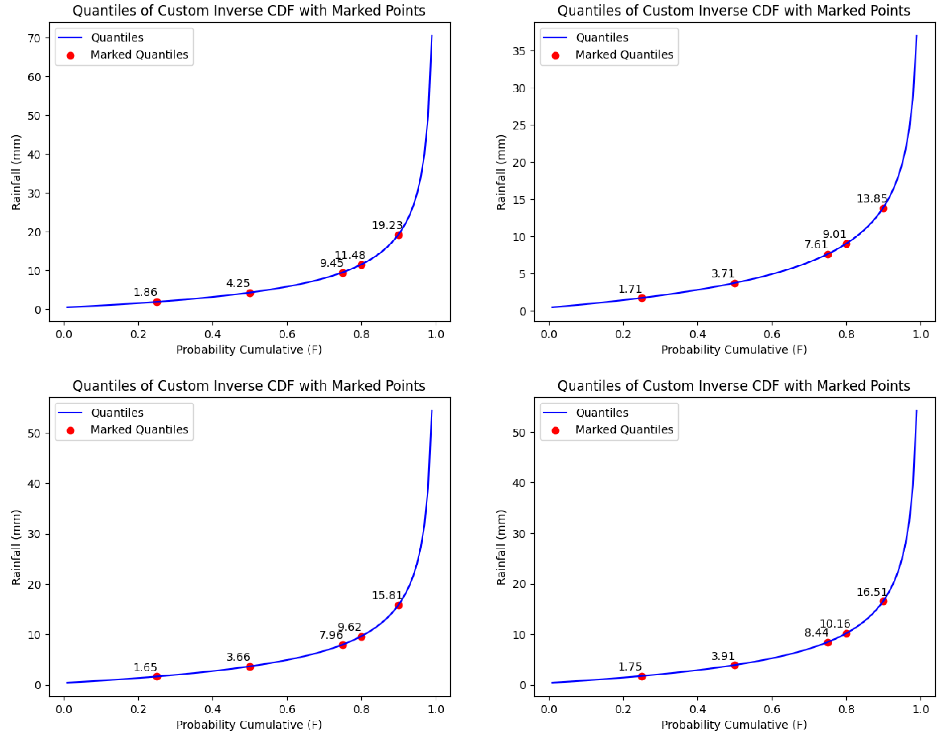
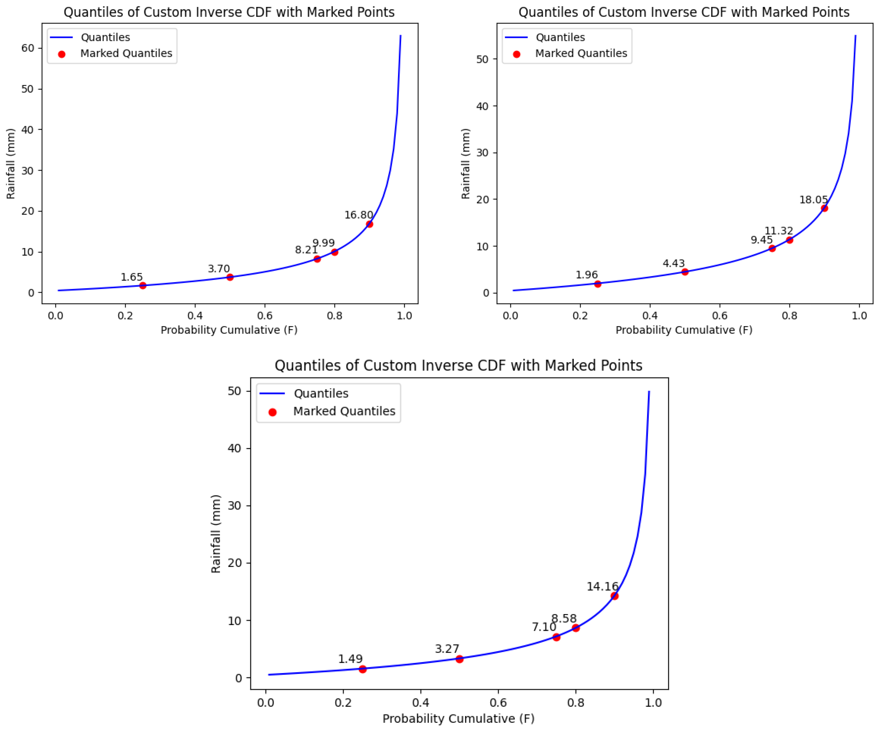
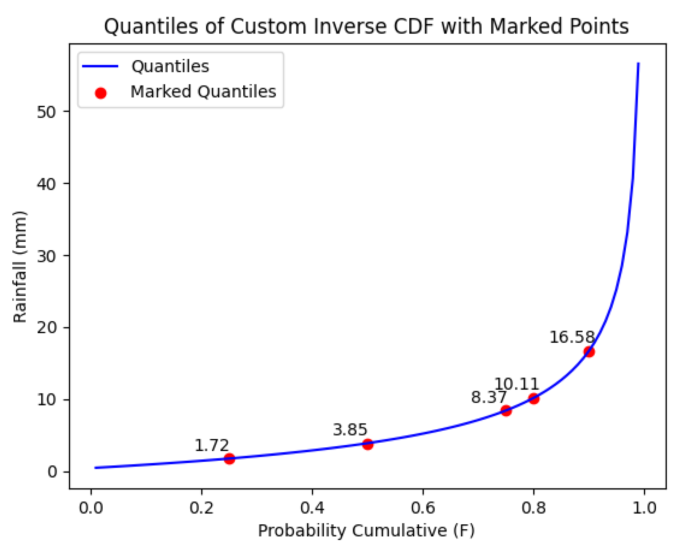
Appendix E. GPA Inverse CDF on Site
References
- Ramos, M. Divisive and hierarchical clustering techniques to analyse variability of rainfall distribution patterns in a Mediterranean region. Atmos. Res. 2001, 57, 123–138. [Google Scholar] [CrossRef]
- IPCC. Climate Change 2023: Synthesis Report (Full Volume) Contribution of Working Groups I, II and III to the Sixth Assessment Report of the Intergovernmental Panel on Climate Change; Core Writing Team, Lee, H., Romero, J., Eds.; IPCC: Geneva, Switzerland, 2023; p. 184. [Google Scholar] [CrossRef]
- Diez-Sierra, J.; del Jesus, M. A rainfall analysis and forecasting tool. Environ. Model. Softw. 2017, 97, 243–258. [Google Scholar] [CrossRef]
- Cassalho, F.; Beskov, S.; de Mello, C.R.; de Moura, M.M. Regional flood frequency analysis using L-moments for geographically defined regions: An assessment in Brazil. J. Flood Risk Manag. 2019, 12, e12453. [Google Scholar] [CrossRef]
- Senent-Aparicio, J.; Soto, J.; Pérez-Sánchez, J.; Garrido, J. A novel fuzzy clustering approach to regionalise watersheds with an automatic determination of optimal number of clusters. J. Hydrol. Hydromech. 2017, 65, 359–365. [Google Scholar] [CrossRef]
- Aragón, L.; Lavado-Casimiro, W.; Montesinos, C.; Zubieta, R.; Laqui, W. Estimación de lluvias extremas mediante un enfoque de análisis regional y datos satelitales en Cusco, Perú. Tecnol. Cienc. Agua 2024, 15, 1–64. [Google Scholar] [CrossRef]
- Smithers, J.; Schulze, R. A methodology for the estimation of short duration design storms in South Africa using a regional approach based on L-moments. J. Hydrol. 2001, 241, 42–52. [Google Scholar] [CrossRef]
- Topçu, E.; Seçkin, N. Drought Analysis of the Seyhan Basin by Using Standardized Precipitation Index SPI and L-moments. J. Agric. Sci. 2016, 22, 196–215. [Google Scholar] [CrossRef]
- Rahman, A.S.; Rahman, A.; Zaman, M.A.; Haddad, K.; Ahsan, A.; Imteaz, M. A study on selection of probability distributions for at-site flood frequency analysis in Australia. Nat. Hazards 2013, 69, 1803–1813. [Google Scholar] [CrossRef]
- Serrano-Notivoli, R.; de Luis, M.; Beguería, S. An R package for daily precipitation climate series reconstruction. Environ. Model. Softw. 2017, 89, 190–195. [Google Scholar] [CrossRef]
- Hosking, J.R.M.; Wallis, J.R. Regional Frequency Analysis: An Approach Based on L-Moments; Cambridge University Press: Cambridge, UK, 1997. [Google Scholar]
- Malekinezhad, H.; Zare-Garizi, A. Regional frequency analysis of daily rainfall extremes using L-moments approach. Atmósfera 2014, 27, 411–427. [Google Scholar] [CrossRef]
- Kjeldsen, T.R.; Smithers, J.C.; Schulze, R.E. Regional flood frequency analysis in the KwaZulu-Natal province, South Africa using the index-flood method. J. Hydrol. 2002, 255, 194–211. [Google Scholar] [CrossRef]
- Vivekanandan, N. Flood frequency analysis using method of moments and L-moments of probability distributions. Cogent Eng. 2015, 2, 1018704. [Google Scholar] [CrossRef]
- Blanco-Gómez, P.; Ortiz-Vallespi, J.; Estrany-Planas, P.; Orihuela-Martínez, J. Rainfall Frequency Analysis (RainFA) Package [Software]. 2023. Available online: https://github.com/vielca/RainFA (accessed on 7 May 2025).
- Blanco-Gómez, P.; Estrany-Planas, P.; Jiménez-García, J.L. Cumulative Rainfall Radar Recalibration with Rain Gauge Data Using the Colour Pattern Regression Algorithm QGIS Plugin. Remote Sens. 2024, 16, 3496. [Google Scholar] [CrossRef]
- Estrany-Planas, P.; Blanco-Gómez, P.; Vilarrasa, V. Aplicación del análisis regional de frecuencias a las series diarias de precipitación usando la metodología de los L-moments en la ciudad de Palma para la caracterización de la lluvia de diseño. In Proceedings of the VII Jornadas de Ingeniería del Agua. La resiliencia de las Infraestructuras Hidráulicas ante el Cambio Climático, 18–19 October, Cartagena, Spain; Universidad Politécnica de Cartagena: Cartagena, Spain, 2023; pp. 359–372. [Google Scholar] [CrossRef]
- Council of European Communities. Council Directive 91/271/EEC of 21 May 1991 Concerning Urban Waste-Water Treatment. 1991. Available online: http://data.europa.eu/eli/dir/1991/271/oj (accessed on 7 May 2025).
- European Parliament and Council of the European Union. Directive (EU) 2024/3019 of the European Parliament and of the Council Concerning Urban Wastewater Treatment (Recast). 2024. Available online: https://eur-lex.europa.eu/legal-content/EN/TXT/?uri=celex:52022PC0541 (accessed on 7 May 2025).
- Ministerio de la Presidencia, Relaciones con las Cortes y Memoria Democrática. Real Decreto 665/2023, de 18 de julio, por el que se Modifica el Reglamento del Dominio Público Hidráulico, Aprobado por Real Decreto 849/1986, de 11 de Abril; el Reglamento de la Administración Pública del Agua, Aprobado por Real Decreto 927/1988, de 29 de julio; y el Real Decreto 9/2005, de 14 de enero, por el que se Establece la Relación de Actividades Potencialmente Contaminantes del suelo y los Criterios y estáNdares para la Declaración de suelos Contaminados. 2023. Available online: https://www.boe.es/diario_boe/txt.php?id=BOE-A-2023-18806 (accessed on 7 May 2025).
- Mann, H.B. Nonparametric Tests Against Trend. Econometrica 1945, 13, 245–259. [Google Scholar] [CrossRef]
- Kendall, M.G. Rank Correlation Methods, 4th ed.; Charles Griffin: London, UK, 1975; pp. 245–259. [Google Scholar]
- The Pandas Development Team. Pandas-dev/Pandas: Pandas 2023. Available online: https://zenodo.org/records/7979740 (accessed on 7 May 2025).
- Wright, D.B.; Mantilla, R.; Peters-Lidard, C.D. A remote sensing-based tool for assessing rainfall-driven hazards. Environ. Model. Softw. 2017, 90, 34–54. [Google Scholar] [CrossRef]
- Hael, M.A.; Yongsheng, Y.; Saleh, B.I. Visualization of rainfall data using functional data analysis. SN Appl. Sci. 2020, 2, 461. [Google Scholar] [CrossRef]
- Hyndman, R.T.; Shang, H.L. Rainbow plots, bagplots, and boxplots for functional data. J. Comput. Graph. Stat. 2010, 19, 29–45. [Google Scholar] [CrossRef]
- Tukey, J.W. Exploratory Data Analysis; Addison Wesley: Reading, PA, USA, 1977. [Google Scholar]
- Wickham, H.; Stryjewski, L. 40 Years of Boxplots. 2011. Available online: http://vita.had.co.nz/papers/boxplots.pdf (accessed on 7 May 2025).
- Hyndman, R.T. Computing and Graphing Highest Density Regions. Am. Stat. 1996, 52, 120–126. [Google Scholar] [CrossRef]
- Searcy, J.K.; Hardison, C.H. Double-Mass Curves. Geol. Surv. Water Supply Pap. 1960, 1541-B, 31–65. [Google Scholar]
- Partal, T.; Kahya, E. Trend analysis in Turkish precipitation data. Hydrol. Process. 2006, 20, 2011–2026. [Google Scholar] [CrossRef]
- Salmi, T.; Määttä, A.; Anttila, P.; Ruoho-Airola, T.; Amnell, T. Detecting Trends of Annual Values of Atmospheric Pollutants by the Mann-Kendall Test and Sen’s Slope Estimates—The Excel Template Application MAKESENS; User Manual; Air Quality, Finish Meteorological Institute: Helsinki, Finland, 2002. [Google Scholar]
- Citakoglu, H.; Minarecioglu, N. Trend analysis and change point determination for hydro-meteorological and groundwater data of Kizilirmak basin. ATheoretical Appl. Climatol. 2021, 145, 1275–1292. [Google Scholar] [CrossRef]
- Blanco-Gómez, P.; Jimeno-Sáez, P.; Senent-Aparicio, J.; Pérez-Sánchez, J. Impact of Climate Change on Water Balance Components and Droughts in the Guajoyo River Basin (El Salvador). Water 2019, 11, 2360. [Google Scholar] [CrossRef]
- Hussain, M.; Mahmud, I. pyMannKendall: A python package for non parametric Mann Kendall family of trend tests. J. Open Source Softw. 2019, 4, 1556. [Google Scholar] [CrossRef]
- Das, S. Extreme rainfall estimation at ungauged sites: Comparison between region-of-influence approach of regional analysis and spatial interpolation technique. Int. J. Climatol. 2019, 39, 407–423. [Google Scholar] [CrossRef]
- Agencia Estatal de Meteorología (AEMET). Valores Climatológicos. 2024. Available online: https://www.aemet.es/es/serviciosclimaticos/datosclimatologicos/valoresclimatologicos (accessed on 7 May 2025).
- Borcard, D.; Gillet, F.; Legendre, P. Numerical Ecology with R; Springer International Publishing AG: Berlin/Heidelberg, Germany, 2011. [Google Scholar] [CrossRef]
- Ward, J.H. Hierarchical grouping to optimize an objective function. J. Am. Statist. Assoc. 1963, 58, 236–244. [Google Scholar] [CrossRef]
- Rousseeuw, P.J. Silhouettes: A Graphical Aid to the Interpretation and Validation of Cluster Analysis. Comput. Appl. Math. 1987, 20, 53–65. [Google Scholar] [CrossRef]
- Arbelaitz, O.; Gurrutxaga, I.; Muguerza, J.; Pérez, J.M.; Perona, I. An extensive comparative study of cluster validity indices. Pattern Recognit. 2013, 46, 243–256. [Google Scholar] [CrossRef]
- Ramachandra Rao, A.; Srinivas, V. Regionalization of watersheds by hybrid-cluster analysis. J. Hydrol. 2006, 318, 37–56. [Google Scholar] [CrossRef]
- Aktürk, G.; Çıtakoğlu, H.; Demir, V.; Beden, N. Meteorological Drought Analysis and Regional Frequency Analysis in the Kızılırmak Basin: Creating a Framework for Sustainable Water Resources Management. Water 2024, 16, 2124. [Google Scholar] [CrossRef]
- Millington, N.; Das, S.; Simonovic, S. The Comparison of GEV, Log-Pearson Type 3 and Gumbel Distributions in the Upper Thames River Watershed Under Global Climate Models. 2011. Available online: https://ir.lib.uwo.ca/wrrr/40 (accessed on 2 June 2025).
- Liu, Z.N.; Yu, X.Y.; Jia, L.F.; Wang, Y.S.; Song, Y.C.; Meng, H.D. The influence of distance weight on the inverse distance weighted method for ore-grade estimation. Sci. Rep. 2021, 11, 2689. [Google Scholar] [CrossRef]
- Achilleos, G. The Inverse Distance Weighted interpolation method and error propagation mechanism—creating a DEM from an analogue topographical map. J. Spat. Sci. 2011, 56, 283–304. [Google Scholar] [CrossRef]
- Sahu, R.; Verma, M.; Ahmad, I. Regional Frequency Analysis Using L-Moment Methodology—A Review; Recent Trends in Civil Engineering; Springer: Singapore, 2021; Volume 77, pp. 811–832. [Google Scholar] [CrossRef]
- Badyalina, B.; Mokhtar, N.A.; Mat Jan, N.A.; Hassim, N.H.; Yusop, H. Flood Frequency Analysis using L-Moment For Segamat River. Matematika 2021, 37, 47–62. [Google Scholar] [CrossRef]
- Zambrano-Bigiarini, M.; Nauditt, A.; Birkel, C.; Verbist, K.; Ribbe, L. Temporal and spatial evaluation of satellite-based rainfall estimates across the complex topographical and climatic gradients of Chile. Hydrol. Earth Syst. Sci. 2017, 21, 1295–1320. [Google Scholar] [CrossRef]
- Jimeno-Sáez, P.; Blanco-Gómez, P.; Pérez-Sánchez, J.; Cecilia, J.M.; Senent-Aparicio, J. Impact Assessment of Gridded Precipitation Products on Streamflow Simulations over a Poorly Gauged Basin in El Salvador. Water 2021, 13, 2497. [Google Scholar] [CrossRef]
- Shapiro, S.S.; Wilk, M.B. An Analysis of Variance Test for Normality (Complete Samples). Biometrika 1965, 52, 591–611. [Google Scholar] [CrossRef]
- Gelabert, M.; Rodríguez-Perea, A. Unidades morfológicas del llano de Palma (Mallorca). In Geomorfología en España; Sociedad Espanola de Geomorfologia: Logrono, Spain, 1994; pp. 403–411. [Google Scholar]
- Torrens Calleja, J.M.; Rosselló Geli, J.; Grimalt Gelabert, M. Recopilación de Información Vinculada a Temporales de Viento, Precipitaciones Torrenciales e Inundaciones en la Ciudad de Palma de Mallorca Entre los Años 2000 y 2015. In Proceedings of the X Congreso Internacional AEC: Clima, Sociedad, Riesgos y Ordenación del Territorio, Alicante, Spain, 5–8 October 2016; pp. 417–425. [Google Scholar]
- Torrens Calleja, J.M. Percepción de las precipitaciones en el Municipio de Palma de Mallorca (Illes Balears) entre 1980–2010. In Análisis Espacial y Representación Geográfica: Innovación y Aplicación; Realidades del Medio fíSico; Universidad de Zaragoza, Departamento de Geografía y Ordenación del Territorio: Zaragoza, Spain, 2015; pp. 1891–1900. [Google Scholar]
- Govern de les Illes Balears. Servei de Mapa de la Pluviometria de Règim Extrem de les Illes Balears. Pluviometria de Règim Extrem (Període de Retorn: 10 Anys). 2024. Available online: https://ideib.caib.es/geoserveis/rest/services/public/GOIB_Meteo_IB/MapServer/5 (accessed on 7 May 2025).
- Gelabert, M. Repartiment de les Precipitacions Màximes a Mallorca; Treballs de Geografía; Universitat de les Illes Balears: Palma, Spain, 1989; Volume 41, pp. 7–18. [Google Scholar]
- Balearsmeteo. Balears Meteo, Network of Amateur Weather Stations in the Balearic Islands. 2024. Available online: http://balearsmeteo.com/ (accessed on 7 May 2025).
- Sevruk, B. Adjustment of tipping-bucket precipitation gauge measurements. Atmos. Res. 1996, 42, 237–246. [Google Scholar] [CrossRef]
- Wagner, P.D.; Fiener, P.; Wilken, F.; Kumar, S.; Schneider, K. Comparison and evaluation of spatial interpolation schemes for daily rainfall in data scarce regions. J. Hydrol. 2012, 464–465, 388–400. [Google Scholar] [CrossRef]
- Das, S.; Millington, N.; Simonovic, S. Distribution choice for the assessment of design rainfall for the city of London (Ontario, Canada) under climate change. Can. J. Civ. Eng. 2013, 40, 121–129. [Google Scholar] [CrossRef]
- Beersma, J.J.; Buishand, T.A. Drought in the Netherlands – Regional frequency analysis versus time series simulation. J. Hydrol. 2007, 347, 332–346. [Google Scholar] [CrossRef]
- Lopes Martins, L.; Souza, J.; Sobierajski, G.; Blain, G. Is it possible to apply the regional frequency analysis to daily extreme air temperature data? Bragantia 2022, 81, e4322. [Google Scholar] [CrossRef]


| Statistic | Equation | Optimal Value |
|---|---|---|
| POD | 1 | |
| FAR | 0 | |
| CSI | 1 | |
| BS | 1 |
| Statistic | Equation | Value Range |
|---|---|---|
| RMSE | ||
| NSE | ||
| PBIAS |
| Type of Event | Daily Rainfall Intensity (mm/day) |
|---|---|
| No rain | <1 |
| Light rain | [1, 5) |
| Moderate rain | [5, 20) |
| Heavy rain | [20, 40) |
| Violent rain | ≥40 |
| Station Name | Series Start Date-Time | Series End Date-Time |
|---|---|---|
| El Pil·lari | 31/12/2015 18:50 | 18/05/2022 23:00 |
| La Bonanova | 12/02/2015 11:30 | 18/05/2022 10:30 |
| Pòrtol | 08/10/2016 10:20 | 11/05/2022 00:00 |
| Son Rapinya | 21/11/2018 14:50 | 11/05/2022 00:00 |
| Pont d’Inca | 23/01/2009 20:00 | 19/05/2022 12:00 |
| Puntiró | 14/01/2017 16:40 | 26/06/2022 22:30 |
| Secar de la Real | 05/02/2021 21:10 | 23/06/2022 19:50 |
| Son Ferriol | 03/05/2021 23:40 | 22/06/2022 15:10 |
| Portopí (B228) | 01/01/2015 00:10 | 01/07/2022 00:00 |
| UIB (B236) | 01/01/2015 00:10 | 01/07/2022 00:00 |
| Aeropuerto (B278) | 01/01/2015 00:10 | 01/07/2022 00:00 |
| Station | s | Var(S) | Z | Trend |
|---|---|---|---|---|
| B228 | −962 | 2.72 | −0.58 | No |
| B236 | −3942 | 4.01 | −1.97 | Decreasing |
| B278 | −1413 | 1.66 | −1.09 | No |
| El Pil·lari | −2213 | 1.38 | −1.88 | No |
| La Bonanova | −3161 | 2.56 | −1.98 | Decreasing |
| Pont d’Inca | 7737 | 1.07 | 2.36 | Increasing |
| Pòrtol | −2297 | 1.64 | −0.90 | No |
| Puntiró | −1156 | 1.02 | −2.27 | Decreasing |
| Secar de la Real | 91 | 3.56 | 0.48 | No |
| Son Rapinya | −835 | 2.47 | −1.68 | No |
| No. | Name | Di | Critical Value | Classification |
|---|---|---|---|---|
| 2 | La Bonanova | 1.08 | 1.92 | Non-discordant |
| 4 | Son Rapinya | 0.60 | 1.92 | Non-discordant |
| 5 | Pont d’Inca | 0.86 | 1.92 | Non-discordant |
| 7 | Secar de la Real | 1.55 | 1.92 | Non-discordant |
| 9 | B228 | 0.76 | 1.92 | Non-discordant |
| 10 | B236 | 1.20 | 1.92 | Non-discordant |
| 11 | B278 | 0.95 | 1.92 | Non-discordant |
| No. | Name | All | Ward Group | W. Group* |
|---|---|---|---|---|
| 1 | El Pil·lari | x | - | - |
| 2 | La Bonanova | x | x | x |
| 3 | Pòrtol | x | - | - |
| 4 | Son Rapinya | x | x | x |
| 5 | Pont d’Inca | x | x | x |
| 6 | Puntiró | x | - | - |
| 7 | Secar de la Real | x | x | x |
| 9 | B228 | x | x | x |
| 10 | B236 | x | x | x |
| 11 | B278 | x | - | x |
| Heterogeneity for different minimum daily precipitation | ||||
| Pd ≥ 0.2 mm | 9.74 | 3.61 | 3.69 | |
| Pd ≥ 0.4 mm | 2.72 | 0.79 | 0.56 | |
| Pd ≥ 1 mm | −0.04 | 0.97 | 0.59 | |
| Pd ≥ 2 mm | −0.66 | 0.37 | 0.14 | |
| Statistic | Value | Performance Rank |
|---|---|---|
| POD | 0.95 | 25° |
| FAR | 0.15 | 13° |
| CSI | 0.81 | 12° |
| BS | 1.11 | 19° |
| Statistic | Value | Performance Rank |
|---|---|---|
| RMSE | 2.86 mm | 25° |
| NSE | 0.86 | 14° |
| PBIAS | −2.49% | 58° |
| Type of Event | Daily Rainfall Intensity (mm/day) | CSI Value | Rank |
|---|---|---|---|
| No rain | <1 mm | 0.84 | 5° |
| Light rain | [1, 5) mm | 0.51 | 1° |
| Moderate rain | [5, 20) mm | 0.62 | 1° |
| Heavy rain | [20, 40) mm | 0.44 | 26° |
| Violent rain | ≥40 mm | 0.7 | 15° |
| GLO | 1.54 |
| GEV | 2.97 |
| GPA | 1.06 |
| PE3 | 3.62 |
| Parameters | |
|---|---|
| GLO | k (shape): −1.103, (scale): 4.708, (location): 3.944 |
| GEV | k (shape): −0.462, (scale): 3.821, (location): 2.894 |
| GPA | k (shape): −0.392, (scale): 4.326, (location): 0.4 |
| PE3 | (shape): 0.321, (scale): 11.91, (location): 0.120 |
| Name | ||||
|---|---|---|---|---|
| GEV | GLO | GPA | PE3 | |
| La Bonanova | 0.95 | 0.61 | 0.46 | 1.38 |
| Son Rapinya | 0.69 | 0.24 | 0.01 | 1.22 |
| Pont d’Inca | 1.32 | 0.84 | 0.57 | 1.69 |
| Secar de la Real | 0.39 | 0.04 | 0.06 | 1.21 |
| B228 | 0.92 | 0.52 | 0.38 | 1.68 |
| B236 | 1.59 | 1.22 | 0.64 | 0.85 |
| B278 | 1.01 | 0.57 | 0.42 | 1.44 |
Disclaimer/Publisher’s Note: The statements, opinions and data contained in all publications are solely those of the individual author(s) and contributor(s) and not of MDPI and/or the editor(s). MDPI and/or the editor(s) disclaim responsibility for any injury to people or property resulting from any ideas, methods, instructions or products referred to in the content. |
© 2025 by the authors. Licensee MDPI, Basel, Switzerland. This article is an open access article distributed under the terms and conditions of the Creative Commons Attribution (CC BY) license (https://creativecommons.org/licenses/by/4.0/).
Share and Cite
Estrany-Planas, P.; Blanco-Gómez, P.; Ortiz-Vallespí, J.I.; Orihuela-Martínez, J.; Vilarrasa, V. Regional Frequency Analysis Using L-Moments for Determining Daily Rainfall Probability Distribution Function and Estimating the Annual Wastewater Discharges. Hydrology 2025, 12, 152. https://doi.org/10.3390/hydrology12060152
Estrany-Planas P, Blanco-Gómez P, Ortiz-Vallespí JI, Orihuela-Martínez J, Vilarrasa V. Regional Frequency Analysis Using L-Moments for Determining Daily Rainfall Probability Distribution Function and Estimating the Annual Wastewater Discharges. Hydrology. 2025; 12(6):152. https://doi.org/10.3390/hydrology12060152
Chicago/Turabian StyleEstrany-Planas, Pau, Pablo Blanco-Gómez, Juan I. Ortiz-Vallespí, Javier Orihuela-Martínez, and Víctor Vilarrasa. 2025. "Regional Frequency Analysis Using L-Moments for Determining Daily Rainfall Probability Distribution Function and Estimating the Annual Wastewater Discharges" Hydrology 12, no. 6: 152. https://doi.org/10.3390/hydrology12060152
APA StyleEstrany-Planas, P., Blanco-Gómez, P., Ortiz-Vallespí, J. I., Orihuela-Martínez, J., & Vilarrasa, V. (2025). Regional Frequency Analysis Using L-Moments for Determining Daily Rainfall Probability Distribution Function and Estimating the Annual Wastewater Discharges. Hydrology, 12(6), 152. https://doi.org/10.3390/hydrology12060152