Baseflow Index Trends in Iowa Rivers and the Relationships to Other Hydrologic Metrics

Abstract

The US state of Iowa has experienced profound historical changes in its streamflow and baseflow. While several studies have noted increasing baseflow and baseflow index (BFI) values throughout the 20th century, analyses quantifying BFI trends in recent years or exploring spatial differences in watersheds marked by varying land use and geologic properties have not been conducted. This study calculated annual values for BFI (and several other hydrologic metrics) using flow records from 42 Iowa stream gauges containing at least 50 years of uninterrupted measurements. While BFI overwhelmingly rose throughout the mid-1900s, circa 1990 it began to level off. In some areas of Iowa (e.g., the southwest), BFI has continued to rise over the past 30 years—albeit at a slower rate; in other regions, it has become stationary or declined. One site failed to follow this trend (Walnut Cr), the only basin to experience large-scale urbanization. Furthermore, BFI demonstrated a strong negative correlation to streamflow flashiness, indicating that rising baseflow has also made Iowa streams less dynamic. BFI was largely independent of overall streamflow. These results may suggest the increased influence of conservation practices and the diminishing impacts of tile drainage on the delivery of water to Iowa’s rivers.

1. Introduction

Streamflow is one of the most important hydrologic processes and has been widely measured throughout the past century [1]. Determining the flow rate of a river or stream provides vital information that can inform stakeholders on numerous challenges related to water resources. Engineering solutions for problems such as flooding [2], water scarcity [3], degradation of ecosystems [4], risks associated with aquatic recreation [5], and impaired water quality [6], rely upon streamflow measurement. Because of its many applications, streamflow’s ubiquity is somewhat unique among environmental variables, as it is measured at most major rivers and often contains uninterrupted records that span several decades [7].

In addition to addressing water resources challenges, streamflow provides valuable insights into a watershed’s hydrology. The flow rates measured at a stream gauge result from many climatic, geologic, and land use properties in the upstream basin, and alterations in these properties have marked effects on downstream flow. As hydrologic processes are increasingly being recognized as nonstationary [8], examining historical streamflow records has been utilized to identify and quantify changes in hydrologic behavior [9,10,11]. Monitoring these changes is vital for understanding how stakeholder decisions influence water transport and informing decision-makers who may be following guidance formulated using outdated hydrologic information.

While investigating a river’s hydrologic changes most often involves examining a gauge’s annual mean, minimum, and maximum streamflow values [10], several other metrics can also be explored to glean additional insights. Baseflow—the flow sustained in a river between wet weather events—is among the most important. Separating streamflow into baseflow and runoff components can reveal changes in water transport occurring through land use alteration [12] or the installation of surface and subsurface drainage systems in urban [13] and rural locales [14]. The baseflow index (BFI) is an associated metric that captures the percentage of overall streamflow that baseflow comprises. While baseflow and BFI are related, their behavior may differ depending on the relative influences of climate and land use change present in a watershed [15,16]. Other metrics, such as stream flashiness or the coefficient of variation of streamflow, involve quantifying streamflow dynamics and variability, which are likewise related to geology and upstream land use [17]. The timing and transport of water to river systems are affected by upstream rainfall patterns, landscape retention, and hydraulic impoundments.

Many additional statistics are available for quantifying streamflow behavior [18,19,20]. However, many studies have noted high levels of interconnectivity among such metrics [21], resulting in information redundancy when a plethora of statistics are used to describe hydrologic alterations in the same stream system [22,23]. It is often the case that changes in upstream catchment properties influence flow behavior in ways that are captured by multiple streamflow parameters simultaneously [24,25]. Moreover, the same causal effects lead to observable historical changes in several hydrologic metrics, especially in landscapes that have seen sweeping and widespread alterations [26].

The US state of Iowa contains one of the most heavily altered landscapes in the world [27], which has had profound effects on its hydrology [28,29]. Much of Iowa’s native prairie and savannah ecosystems have been converted to agricultural row crops and pastureland. The most substantial land use conversions occurred in the late 1800s and early 1900s—largely before the advent of robust, long-term streamflow monitoring, but significant changes in streamflow behavior would undoubtedly be evident if such records were available. Over the past half-century, large amounts of subsurface tile drainage have been installed to facilitate quicker delivery of water to streams [30]. In more recent decades, conservation practices have been adopted to detain water upstream and offset the previous alterations that have expedited water’s delivery to streams [31,32]. Along with climate change [33], these factors have resulted in considerable nonstationarity in Iowa’s streamflow records [34]. Iowa’s widespread landscape alterations, along with the many types of geologic properties it encompasses, have made the state an ideal location for exploring changes in streamflow, baseflow, and related hydrologic metrics.

The most widely noted shifts in the state’s hydrology include a gradual rise in minimum and mean streamflow records [35,36,37]. Trend analyses exploring the past 70+ years have demonstrated increasing low-flow periods [38,39], along with higher overall streamflow in Iowa’s rivers [35]. Studies exploring baseflow have found that baseflow rose in most of the state’s major watersheds over the latter half of the 20th century [40]. Indeed, increases in baseflow and BFI represent the most appreciable changes in Iowa’s hydrology in modern times [12,41,42]. While these trends align with broader trends observed in the US Midwest [43,44,45], a thorough examination of BFI and baseflow that incorporates discharge measurements up to the present day and investigates spatial differences in Iowa’s regions has not been conducted. Herein, we updated BFI trend analyses by performing them on nearly all of Iowa’s streamflow records up to the present day. We then examined any potential temporal changes at a high-resolution (i.e., comparing more recent BFI behavior to that of the 20th century). While multiple studies have noted relationships between streamflow and baseflow patterns and trends of other hydrologic metrics at a national scale [10,46], this has not been formally examined within the context of Iowa’s hydrologic history.

In this study, we explored temporal and spatial BFI patterns in Iowa’s rivers and streams. Our primary goals were to (1) calculate annual values for BFI and other hydrologic parameters at several Iowa stream gauges with ample historical data, (2) explore temporal trends of these hydrologic metrics, (3) investigate the interconnectivity between BFI and the other hydrologic parameters, (4) and aggregate BFI values on a statewide scale for Iowa. We were particularly interested in examining BFI over the most recent 30 years (1995–2024) and comparing BFI behavior over this timeframe to the increasing baseflow trends noted from the second half of the 20th century [40].

2. Materials and Methods

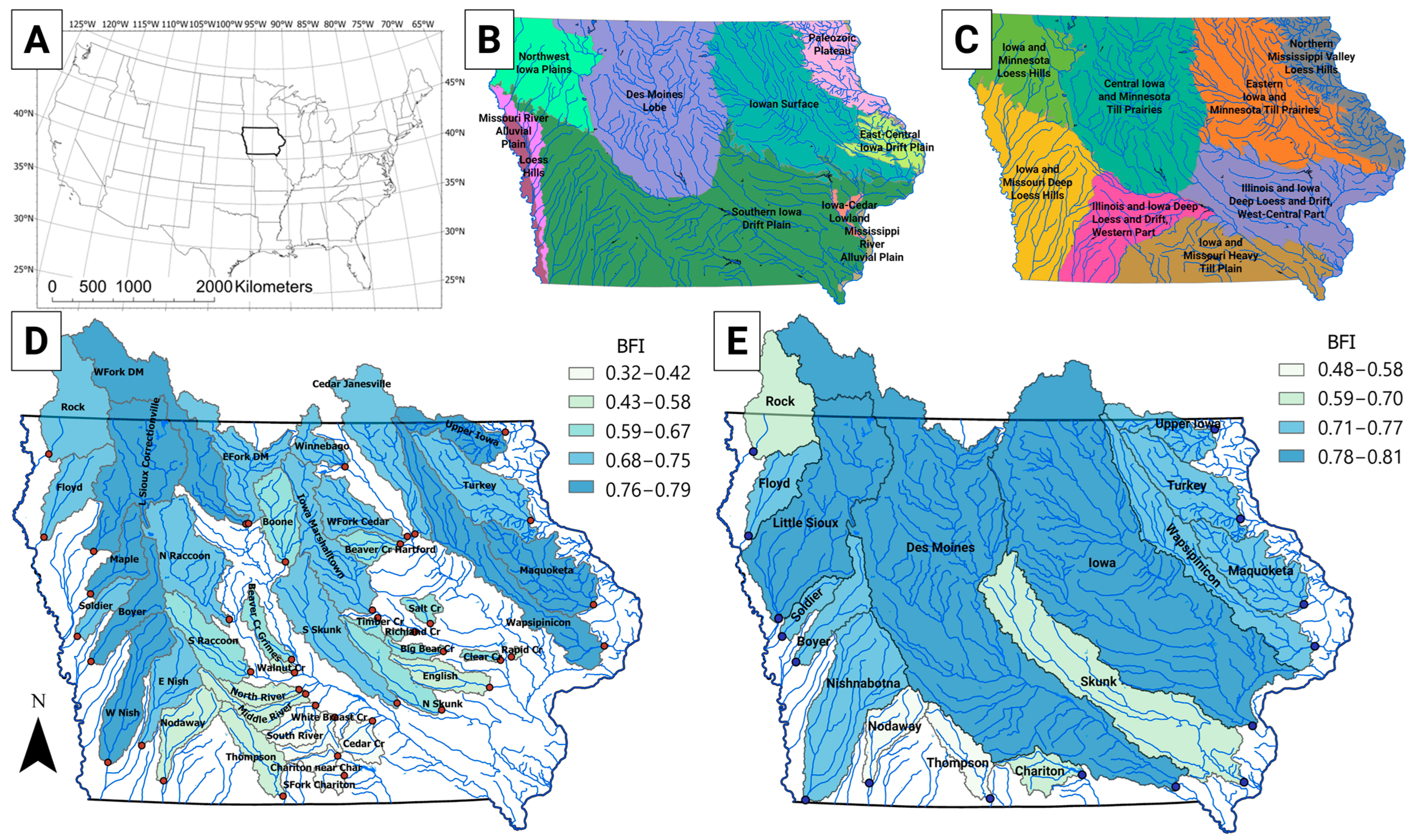
2.1. Regional Setting

The midwestern state of Iowa is located in the heart of the US cornbelt (Figure 1A). The region is characterized by a humid continental climate marked by prominent seasonal behavior, with summers that are typically hot and humid and winters that are relatively cold and dry. Average annual precipitation ranges from approximately 650–1000 mm/year and follows a gradient with lower rainfall totals in the northwest part of the state and greater rainfall in the southeast.

Iowa’s surficial geology mainly consists of glacial deposits containing fine-textured till and loess of various ages overlying flay-lying Paleozoic sedimentary bedrock. The landform regions of Iowa (Figure 1B) were delineated to capture similar types of surficial geology and terrain features present in the state [47]. Among these, the Des Moines Lobe captures Iowa’s most recent glacial advance (~12,000 years ago) in the north-central portion of the state. This landform region is marked by low levels of topographic relief, leading to poor surficial drainage. Artificial drainage systems, including networks of pattern tiles and drainage ditches, dominate the Des Moines Lobe’s modern landscape. The landscapes of southern and southwestern Iowa are characterized by steep, rolling hillslopes with a much greater degree of overland drainage. This region’s soil contains varying depths of fine-textured silt (wind-blown loess) and older glacial till. Northeast Iowa contains fewer glacial deposits and is instead characterized by shallow carbonate bedrock with incised river channels and karst topography. The landform regions are closely related to the major land resource areas (MLRA, Figure 1C), which have traditionally been used by the US Department of Agriculture to group areas by similar patterns in soils, climate, water resources, and land uses [48].

Modern land use in Iowa is predominantly agricultural (>80%), with most of this land (~70%) dedicated to corn and soybean cultivation. Iowa is also home to several prominent livestock industries, and the state is a leader in hog, cattle, and poultry production [49]. Livestock are primarily reared in concentrated animal feeding operations, and these are especially common in the north-central and northwest regions of the state [50]. Over the past several decades, large swaths of pastureland have been converted into cropland, and Iowa’s remaining pastures are predominantly located in the state’s southern half. The large agricultural footprint in Iowa is due to favorable climatic conditions that enable rain-fed crop cultivation and productive soils resulting from glacial deposits. Forested areas comprise ~8% of Iowa’s land area, with deciduous forests being the most common. Wetlands make up ~2% of Iowa, while open waters are <1% of the state’s area.

While urban and suburban areas have experienced significant growth over the past century, they remain a small minority (~5%) of Iowa’s overall land area. Many of the state’s largest metropolitan areas (e.g., Des Moines, Cedar Rapids, and Sioux City) have expanded over the past several decades through urban sprawl, a process that typically involves developing land long dedicated to agriculture. Iowa’s urban and suburban areas contain most of its point source discharges, mainly municipal wastewater treatment plants and industrial factories. Point source effluent can be a major component of streamflow in a handful of small, urban watersheds, but in Iowa’s major rivers, its long-term contribution has typically been <5% of overall streamflow. Certain municipalities routinely draw water from nearby rivers, and some of the most common users include drinking water providers, industrial factories, and data centers. The impact of these facilities on streamflow is generally minor, but concerns about water use can arise during prolonged low-flow periods.

Iowa’s history has been defined by widescale land use change, and very few of the prairies and wetlands that once dominated the native landscape remain. Modern Iowa contains one of the most heavily altered and engineered landscapes in the world, and these alterations have had a profound impact on the state’s hydrologic processes [37,40]. Changes in Iowa’s streamflow profiles have been noted as among the highest in the nation [26]. Due to rainfall and land use practices, water yields tend to be highest in Iowa’s eastern watersheds. Most of Iowa’s waterbodies are gaining systems—consistently fed water via groundwater discharge. Likewise, most major rivers are perennial, with flow continuously supplied through baseflow contributions and effluent from tile lines and point sources. Irrigation in Iowa remains rare, but some center-pivot irrigation systems are deployed in the drier parts of the state (i.e., the western border and northwest region).

2.2. Selection of Stream Gauges

Streamflow in the US has historically been measured using a network of stream gauges owned and operated by the US Geological Survey (USGS). Approximately 140 of such gauges are currently operational in Iowa. Among these 140, we sought to analyze a subset that could be utilized to effectively explore historical BFI changes throughout the state. The following criteria were used to select gauges in our regional analysis of hydrologic trends, and a full framework diagram describing this study’s workflow of retrieving streamflow data and performing subsequent trend analyses has been included in the Supplementary Materials.

First, the gauge needed to contain at least 50 years of continuous streamflow measurements. In other words, a gauge must have commenced its daily streamflow measurements in 1975 or earlier and continued operating continuously until the end of 2024 (the most recent complete calendar year at the time of publication). Several decades of historical hydrologic data are usually necessary to adequately evaluate temporal trends and capture the full range of hydrologic conditions that occur in a river system [51]. A benchmark of 50 years of continuous records was chosen to, at a minimum, enable the comparison of the past 30 years to the increasing baseflow conditions noted in the later decades of the 20th century [40]. It was also critical that gauges were continuously operational throughout this period. At some gauges, the USGS ceased measuring streamflow for years or decades and then restarted their operations at a later date. In these instances, only streamflow values measured since the recommencement of operations were included. Utilizing continuous records enables more robust assessments of historically hydrologic behavior.

Secondly, only gauges located along free-flowing rivers and streams with minimal upstream hydraulic impoundments were selected. Iowa contains several large reservoirs whose release rates are primarily dictated by operator decisions rather than upstream hydrologic processes. The selection gauges on free-flowing waterways allowed for exploring hydrologic changes that were more indicative of climatic and land use changes. Finally, all chosen gauges contained distinct drainage areas. Numerous stream gauges are located on Iowa’s major rivers, and many contain large amounts of overlapping tributary area. For example, two gauges are stationed about 15 km apart along the Iowa River near its mouth. The downriver gauge shares 98% of its drainage area with the upstream site, and any analysis including both sites would largely describe the same hydrologic tendencies. To ensure that no land areas were counted twice in our procedures, we only selected sites that were not nested within the same watershed. In practice, this meant selecting gauges in more upstream parts of a watershed to maximize the number of sites included in our analysis. In situations where a basin contained two viable gauges, the further downstream site was chosen to maximize our study’s land area coverage.

In total, 42 stream gauges were selected for our regional exploration of BFI trends. These gauges’ watersheds cover every major component of geologic, climatic, and land use activity in Iowa and thus widely capture the heterogeneity of Iowa’s hydrology. The only limitation among the selected gauges is that none solely contain urban or suburban areas. This is due to agricultural activities dominating Iowa’s overall landscape and all of its large watersheds. The handful of gauges located in smaller urban watersheds were mostly installed within the past 20 years—limiting our ability to assess hydrologic trends at these sites.

Table 1. USGS stream gauges used in this study. Footnotes specify which gauges were included in the regional and statewide analyses. Start Year refers to the first calendar year in which daily streamflow measurements have been collected continuously through 2024. The BFI column contains the baseflow percentage at each site from the past 50 years (1975–2024); these values were used to color-code Figure 1D,E.

Short Name	USGS Site Name	USGS ID	Area (km2)	Lat	Long	Start Year	BFI (1975–2024)
Beaver Cr Grimes A	Beaver Creek near Grimes, IA	05481950	927	41.6883	−93.7347	1961	0.654
Beaver Cr Hartford A	Beaver Creek at New Hartford, IA	05463000	899	42.5720	−92.6183	1946	0.671
Big Bear Cr A	Big Bear Creek at Ladora, IA	05453000	490	41.7494	−92.1821	1946	0.641
Boone A	Boone River near Webster City, IA	05481000	2186	42.4320	−93.8059	1940	0.647
Boyer A,B	Boyer River at Logan, IA	06609500	2256	41.6417	−95.7823	1938	0.749
Cedar Cr A	Cedar Creek near Bussey, IA	05489000	969	41.2190	−92.9085	1948	0.382
Cedar Janesville A	Cedar River at Janesville, IA	05458500	4302	42.6483	−92.4652	1946	0.719
Chariton B	Chariton River near Rathbun, IA	06903900	1422	40.8219	−92.8913	1957	0.625
Chariton near Char A	Chariton River near Chariton, IA	06903400	471	40.9519	−93.2598	1966	0.334
Clear Cr A	Clear Creek near Coralville, IA	05454300	254	41.6767	−91.5988	1953	0.612
Des Moines B	Des Moines River at Keosauqua, IA	05490500	36,358	40.7278	−91.9596	1912	0.783
E Nish A	East Nishnabotna River at Red Oak, IA	06809500	2315	41.0086	−95.2417	1937	0.708
EFork DM A	East Fork Des Moines River at Dakota City, IA	05479000	3388	42.7236	−94.1935	1940	0.744
English A	English River at Kalona, IA	05455500	1487	41.4697	−91.7146	1940	0.560
Floyd A,B	Floyd River at James, IA	06600500	2295	42.5767	−96.3114	1935	0.745
Iowa B	Iowa River at Wapello, IA	05465500	32,375	41.1781	−91.1821	1915	0.806
Iowa Marshalltown A	Iowa River at Marshalltown, IA	05451500	3968	42.0658	−92.9077	1933	0.733
L Sioux Correctionville A	Little Sioux River at Correctionville, IA	06606600	6475	42.4822	−95.7926	1937	0.778
Little Sioux B	Little Sioux River near Turin, IA	06607500	9132	41.9650	−95.9723	1958	0.791
Maple A	Maple River at Mapleton, IA	06607200	1733	42.1569	−95.8100	1942	0.763
Maquoketa A,B	Maquoketa River near Maquoketa, IA	05418500	4022	42.0834	−90.6329	1914	0.767
Middle River A	Middle River near Indianola, IA	05486490	1268	41.4242	−93.5874	1940	0.553
N Raccoon A	North Raccoon River near Jefferson, IA	05482500	4193	41.9879	−94.3771	1940	0.696
N Skunk A	North Skunk River near Sigourney, IA	05472500	1891	41.3008	−92.2046	1946	0.624
Nishnabotna B	Nishnabotna River above Hamburg, IA	06810000	7268	40.6017	−95.6450	1929	0.763
Nodaway A,B	Nodaway River at Clarinda, IA	06817000	1974	40.7433	−95.0142	1937	0.585
North River A	North River near Norwalk, IA	05486000	904	41.4579	−93.6550	1940	0.577
Rapid Cr A	Rapid Creek near Iowa City, IA	05454000	66	41.7000	−91.4877	1938	0.576
Richland Cr A	Richland Creek near Haven, IA	05451900	145	41.8994	−92.4744	1950	0.632
Rock A,B	Rock River near Rock Valley, IA	06483500	4123	43.2144	−96.2945	1949	0.705
S Raccoon A	South Raccoon River at Redfield, IA	05484000	2574	41.5904	−94.1512	1940	0.670
S Skunk A	South Skunk River near Oskaloosa, IA	05471500	4235	41.3557	−92.6574	1946	0.710
Salt Cr A	Salt Creek near Elberon, IA	05452000	521	41.9642	−92.3132	1946	0.642
SFork Chariton A	South Fork Chariton River near Promise City, IA	06903700	435	40.8006	−93.1924	1968	0.317
Skunk B	Skunk River at Augusta, IA	05474000	11,168	40.7537	−91.2771	1915	0.679
Soldier A,B	Soldier River at Pisgah, IA	06608500	1054	41.8305	−95.9314	1940	0.738
South River A	South River near Ackworth, IA	05487470	1191	41.3372	−93.4863	1940	0.420
Thompson A,B	Thompson River at Davis City, IA	06898000	1816	40.6403	−93.8083	1942	0.485
Timber Cr A	Timber Creek near Marshalltown, IA	05451700	306	42.0089	−92.8524	1950	0.661
Turkey A,B	Turkey River at Garber, IA	05412500	4002	42.7400	−91.2618	1933	0.738
Upper Iowa A,B	Upper Iowa River near Dorchester, IA	05388250	1994	43.4211	−91.5088	1975	0.770
W Nish A	West Nishnabotna River at Randolph, IA	06808500	3434	40.8731	−95.5803	1949	0.788
Walnut Cr A	Walnut Creek at Des Moines, IA	05484800	203	41.5872	−93.7033	1972	0.577
Wapsipinicon A,B	Wapsipinicon River near De Witt, IA	05422000	6050	41.7670	−90.5349	1935	0.750
WFork Cedar A	West Fork Cedar River at Finchford, IA	05458900	2191	42.6294	−92.5435	1946	0.726
WFork DM A	Des Moines River at Humboldt, IA	05476750	5843	42.7194	−94.2205	1965	0.789

^A upstream watershed used for regional analysis. ^B terminal monitoring site used for statewide analysis.

lists these 42 sites and their USGS identifying information and drainage areas. It also contains the earliest year in which continuous streamflow data are available (the Start Year column). All stream gauges used in this study follow standard USGS flow measurement protocols. These include measuring river stage at 15 min increments and converting these observations into corresponding streamflow values using a site-specific stage-discharge rating curve. Daily mean streamflow values are then calculated by taking arithmetic means of the high-resolution flows. In certain circumstances (usually during the winter), flow measurements may be disrupted due to freezing conditions or equipment malfunction. When this occurs, daily streamflow values are retroactively estimated using USGS hydrologic models [52]. Consequently, these sites’ records contain streamflow values approved via USGS’s quality control procedures for nearly every day.

2.3. Calculation of Hydrologic Metrics

Daily mean streamflow values for the selected stream gauges were retrieved using the data retrieval Python package [53]. In rare cases (<0.01% of days), missing flow values were interpolated, with no period of missing values spanning more than four days. Daily water yields (using units of mm/day) were also calculated—a process that involves converting daily flows into their corresponding volumes and then dividing by a site’s tributary area. Water yields allow for better hydrologic comparisons among watersheds of various sizes by normalizing flows using sites’ tributary area. All daily mean streamflow values and water yields have been included in the Supplementary Materials.

2.3.1. Baseflow Separation

Baseflow separation was conducted on the daily USGS streamflow records using the one-parameter recursive digital filter method [54]. Specifically, this study utilized the Lynn–Hollick filter, which deploys the following algorithm on daily streamflow timeseries

$${\mathrm{b}}_{\mathrm{i}}=\propto \ast {\mathrm{b}}_{\mathrm{i}-1}+{\displaystyle \frac{1-\propto }{2}}\ast ({\mathrm{q}}_{\mathrm{i}}-{\mathrm{q}}_{\mathrm{i}-1})$$

(1)

where q_i is the mean streamflow for day i, b_i is the baseflow for day i, and α is the filter parameter. Daily baseflow values are subject to the condition 0 ≤ b_i ≤ q_i. This study used an α value of 0.925, as a filter parameter of 0.925 has proven effective at separating baseflow in perennial midwestern rivers and streams [43,55,56].

Daily BFI values were then obtained by simply dividing a site’s daily baseflow record by its daily streamflow (i.e., BFI_i = b_i/q_i). All BFI values have also been included in the Supplementary Materials. BFI can be estimated for longer timeframes by dividing the summed baseflow volumes by the summed streamflow volumes. To provide context for typical long-term BFI values in Iowa obtained using the Lynn–Hollick filter, we calculated each site’s BFI from 1975–2024, as 1975 was the most recent year where each gauging began maintaining continuous records. These values are listed in the BFI column of Table 1 and were used to form the color-coding scheme in Figure 1D,E.

2.3.2. Annual Statistics

Various hydrologic metrics were calculated at all sites for each calendar year. A focus on annual periods is often advantageous for analyses of hydrologic data, as it eliminates the seasonality routinely present in midwestern streamflow data [57]. Yearly streamflow and baseflow water yields were found by aggregating the daily streamflow and baseflow yields, respectively. BFI for a given calendar year k is formally defined as

$${\mathrm{B}\mathrm{F}\mathrm{I}}_{\mathrm{k}}={\displaystyle \frac{{\sum }_{\mathrm{i}=\mathrm{J}\mathrm{a}\mathrm{n}1,\mathrm{k}}^{\mathrm{D}\mathrm{e}\mathrm{c}31,\mathrm{k}}{\mathrm{b}}_{\mathrm{i}}}{{\sum }_{\mathrm{i}=\mathrm{J}\mathrm{a}\mathrm{n}1,\mathrm{k}}^{\mathrm{D}\mathrm{e}\mathrm{c}31,\mathrm{k}}{\mathrm{q}}_{\mathrm{i}}}}$$

(2)

This is equivalent to the summation of a year’s baseflow divided by a summation of its streamflow.

Several other statistics were calculated using the daily streamflow yields that have often been used to describe hydrologic trends and flow dynamics [18]. These included traditional descriptive statistics of the yearly arithmetic mean (mean) and standard deviation (std), and the coefficient of variation (CV) was found by dividing the annual std by the annual mean. Yearly skewness (skew; i.e., the third statistical moment) was also calculated, along with each river’s annual minimum (min), median, and maximum (max) daily mean streamflow yield.

Annual stream flashiness was calculated using the Richards–Baker flashiness index (RB), which quantifies flashiness by dividing changes in daily streamflow by a river’s total flow [58]. RB metrics for a calendar year were found using the following equation

$$\mathrm{R}\mathrm{B}={\displaystyle \frac{{\sum }_{\mathrm{i}=\mathrm{J}\mathrm{a}\mathrm{n}1,\mathrm{k}}^{\mathrm{D}\mathrm{e}\mathrm{c}31,\mathrm{k}}\left|{\mathrm{q}}_{\mathrm{i}}-{\mathrm{q}}_{\mathrm{i}-1}\right|}{{\sum }_{\mathrm{i}=\mathrm{J}\mathrm{a}\mathrm{n}1,\mathrm{k}}^{\mathrm{D}\mathrm{e}\mathrm{c}31,\mathrm{k}}{\mathrm{q}}_{\mathrm{i}}}}$$

(3)

The RB index has widely been used to describe a stream’s volatility or propensity to change flow rates over short periods [59,60], and a larger RB value indicates a higher degree of flashiness.

An additional metric, Top Days (TD), was also introduced. TD quantifies the percentage of a river’s streamflow that occurs within its wettest days. The equation for calculating TD for a calendar year is

$${\mathrm{T}\mathrm{D}\left(\mathrm{D}\right)}_{\mathrm{k}}={\displaystyle \frac{\sum _1^{\mathrm{D}}{\mathrm{m}\mathrm{a}\mathrm{x}}_{\mathrm{D}}\left(\mathrm{q}\right)}{{\sum }_{\mathrm{i}=\mathrm{J}\mathrm{a}\mathrm{n}1,\mathrm{k}}^{\mathrm{D}\mathrm{e}\mathrm{c}31,\mathrm{k}}{\mathrm{q}}_{\mathrm{i}}}}$$

(4)

where D is the number of maximum flow days to include in the calculation, e.g., for D = 4, the TD metric sums the flows from the four wettest days in a calendar year and divides this by the year’s total streamflow. Therefore, TD is always a percentage bounded between 0.0 and 1.0. TD metrics were calculated using D values of 1, 4, and 37, which roughly correspond to the maximum, 99, and 90 streamflow percentiles over the period of 365 days. A similar statistic has been used to quantify trends in extreme rainfall events [61] and was recently used in an exploration of the relationships between streamflow statistics and flood damages [62].

Upon calculating the annual metrics, a LOESS (locally estimated scatterplot smoothing) algorithm was applied to each timeseries to highlight long-term hydrologic behavior. Such smoothing algorithms reduce the annual variance of observed hydrologic parameters and have routinely been utilized in many explorations of streamflow-related trends [63,64,65]. The specific LOESS algorithm used in this study was implemented using the statsmodel Python package [66] and used values spanning a 30-year window with three iterations of smoothing. Figure 2 illustrates several annual metrics (streamflow yield, baseflow yield, BFI, CV, and RB) and their corresponding LOESS lines at an example site (Floyd). This study’s Supplementary Materials contain similar plots for all 42 selected stream gauges, along with values for all annual hydrologic metrics and LOESS lines.

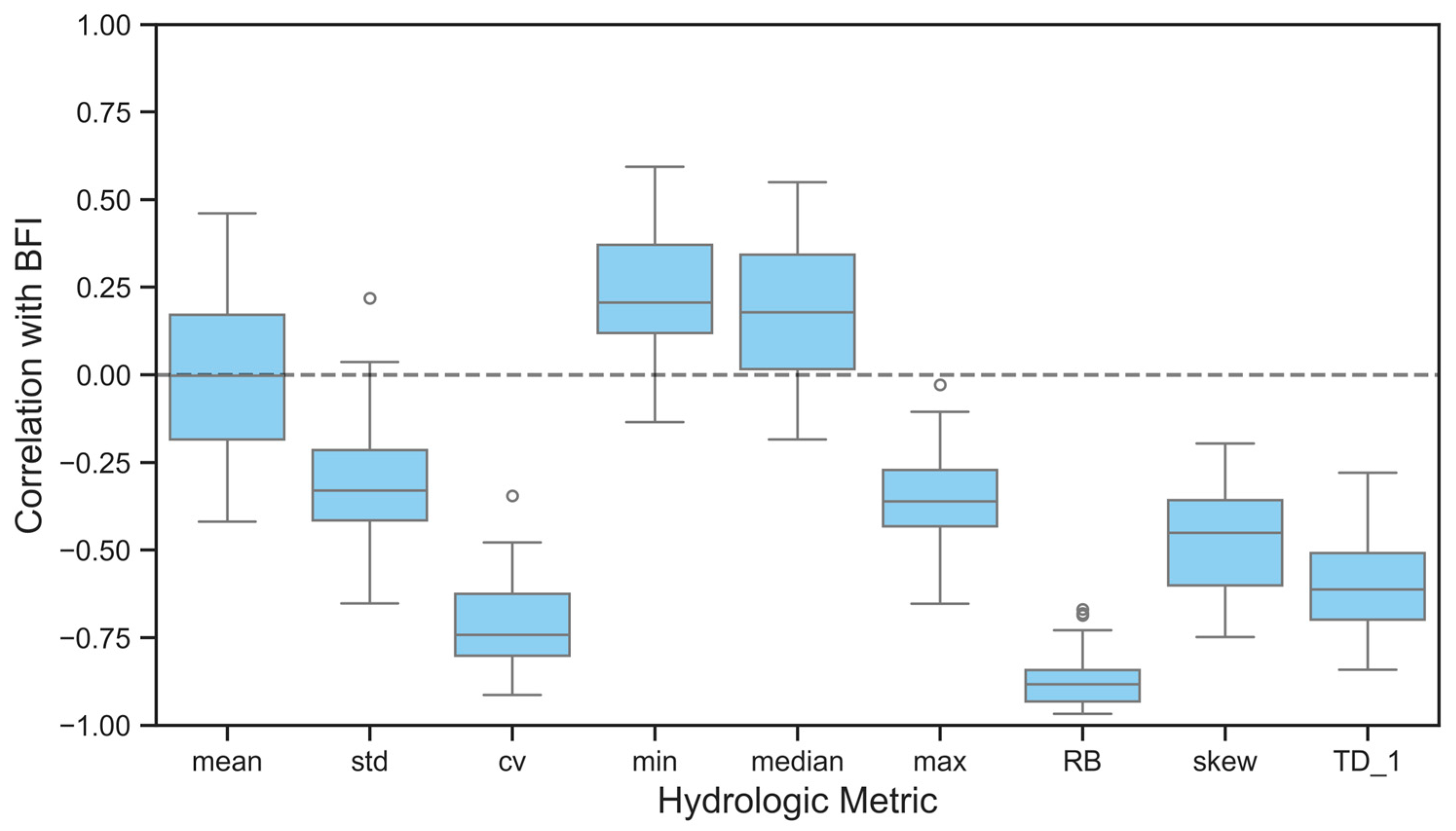
2.3.3. Correlations Between BFI and Other Metrics

Scatterplots were created to investigate the relationships between BFI and the hydrologic metrics in these river systems that plotted each site’s suite of hydrologic metrics against annual BFI (Supplementary Materials). Pearson correlation coefficients were also calculated to quantify the strength of these relationships, e.g., calculating the correlation between the BFI and CV values shown in Figure 2. Boxplots were created to summarize the correlation coefficients across the 42 gauges.

2.4. Trend Analysis

Temporal changes in hydrology were formally analyzed using a modified version of the Mann–Kendall monotonic trend test that accounts for positive autocorrelation within hydrologic datasets [67]. This nonparametric statistical test has proven effective at evaluating long-term behavior in streamflow [68] and baseflow [43]. In addition to calculating a p-value associated with trend significance, trend magnitude was also estimated using the Theil–Sen method, where a slope across the duration of the analysis period is quantified [69,70]. These tests were conducted for all annual timeseries of hydrologic metrics at the 42 regional sites, and all trend analyses were performed using the pymannkendall Python package [71].

Furthermore, to investigate changing hydrologic behavior at a higher temporal resolution, we subdivided the historical analysis period into three distinct 30-year periods: (1) 1935–1964, (2) 1965–1994, and (3) 1995–2024. Increments of 30 years are widely used in climatic analyses [72,73], and organizing timeframes in this manner allowed us to explore differences in trends that may have occurred throughout the past 90 years. The aforementioned trend test was performed on each of the 30-year periods for the 42 sites—the only exception being the 1935–1964 window for 12 gauges with insufficient data. Trends for this period were not evaluated for gauges that became operational after 1946, as we set a threshold of a timeframe needing at least 20 years of data for a trend test to be performed. The complete results of our trend analysis, including the slopes and p-values for the full analysis period and 30-year windows, have been included in the Supplementary Materials.

2.5. Statewide Analysis

To estimate BFI values for the state of Iowa, streamflow and baseflow volumes were aggregated from 16 gauges located along Iowa’s major rivers near its border (Figure 1E). These gauges represent the furthest downstream points within Iowa where each river’s streamflow is monitored. Their collective drainage area encompasses over 90% of Iowa’s land area, and thus, they effectively capture most hydrologic, geologic, and land use behavior in the state. Similar sets of sites (often called terminal sites) have been used to quantify streamflow behavior or pollutant loads for Iowa as a whole [74,75,76,77].

Table 1 lists the specific gauges used for the statewide totals, several of which were also included in the regional analysis. Each of these gauges has been operational for at least the last 50 years, and 14 of the 16 have data extending back to 1950. Consequently, 1950 was the earliest year in which we aggregated statewide flows. Annual streamflow and baseflow values were calculated for each site using the aforementioned methods, and these values were then summed for the 16 sites to generate Iowa’s overall streamflow and baseflow. Statewide yields were determined by dividing statewide streamflow and baseflow by the combined area of the 16 terminal sites, and statewide BFI values were found by dividing Iowa’s overall baseflow by its overall streamflow (Supplementary Materials). It should be noted that the calculation of statewide streamflow, baseflow, and BFI is possible since these values are found by aggregating water volumes together. Statewide versions of other metrics used in this study (e.g., CV, skew, and RB) are not feasible because they are statistical descriptions of streamflow behavior at a specific gauge and, therefore, do not lend themselves to aggregation across multiple streams.

3. Results

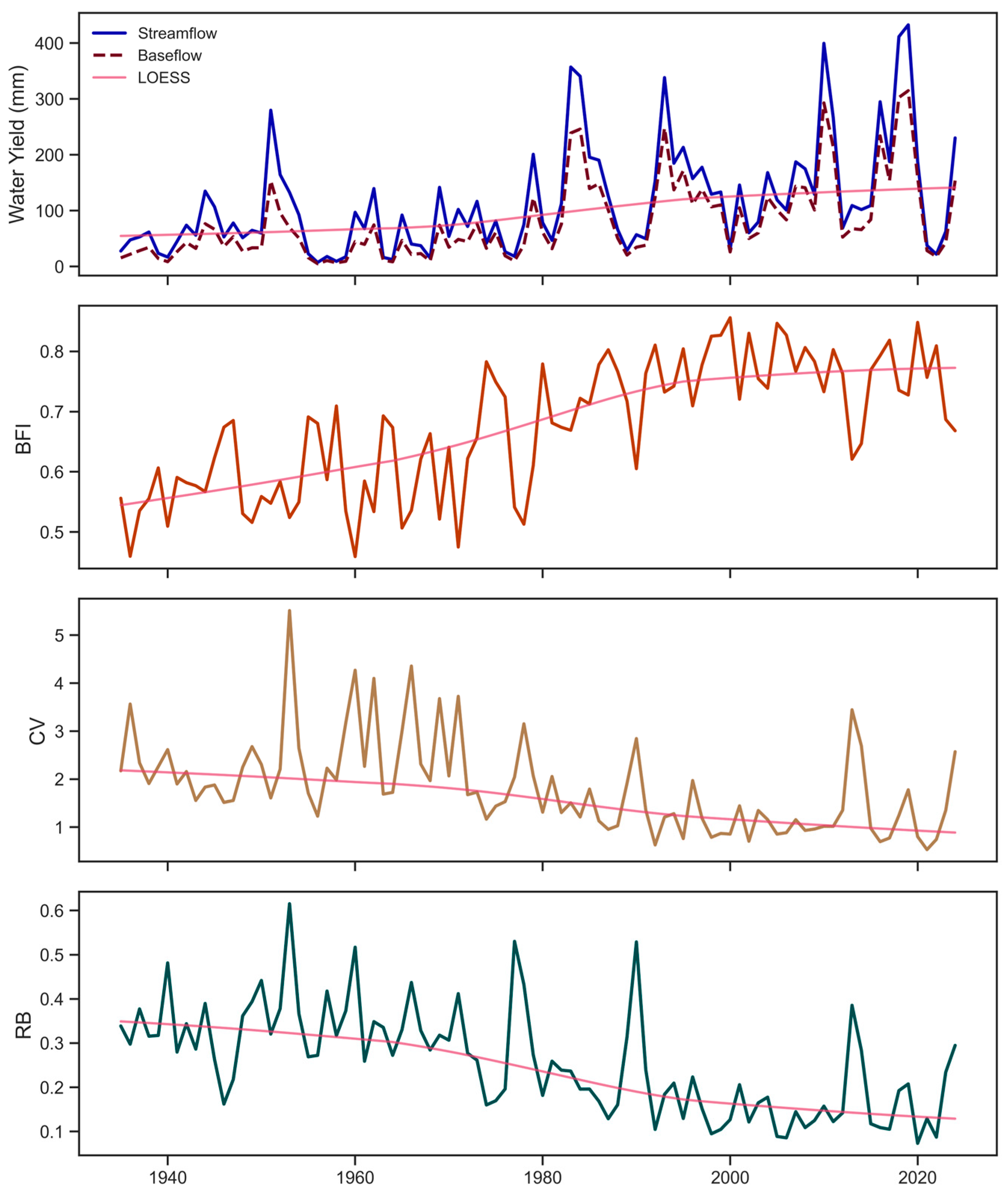
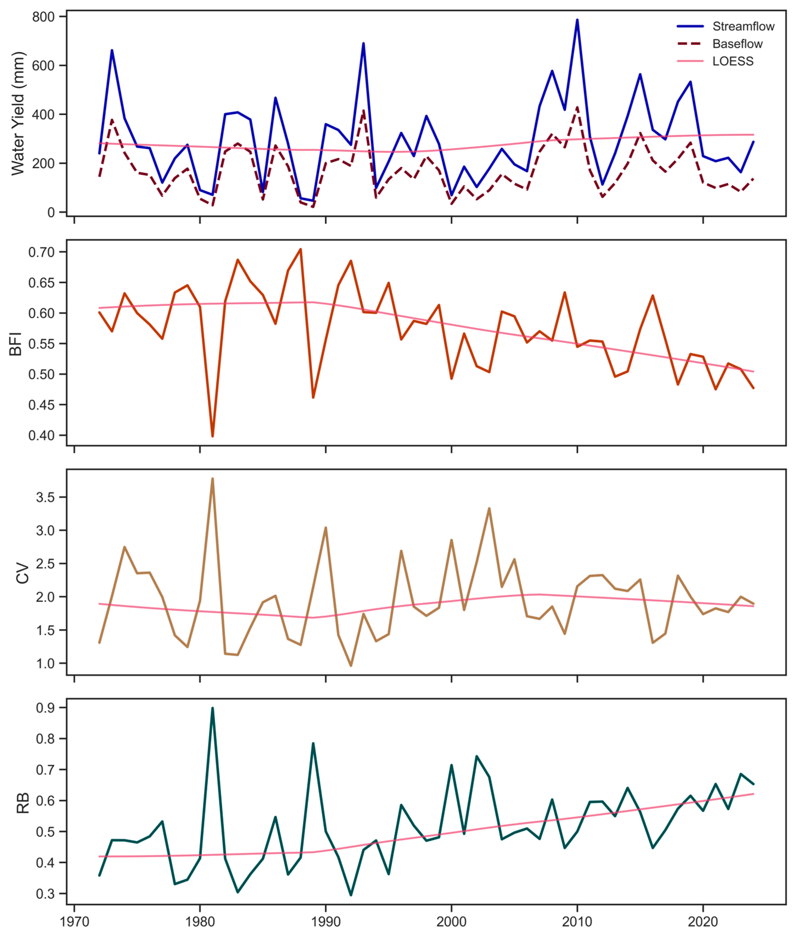
3.1. Hydrologic Metrics

All annual hydrologic metrics were calculated for each gauge. The complete list of calculated metrics included streamflow yield, baseflow yield, BFI, mean, std, CV, min, median, max, skew, RB, TD (1), TD (4), and TD (37). In general, there was great variation among the annual values, both from year to year and between gauges.

Table 2. Statistical summary of the annual hydrologic metrics.

Stat	Flow	Baseflow	BFI	Mean	Std	CV	Min	Median	Max	Skew	RB	TD1	TD4	TD37
mean	222	138	0.629	0.602	1.08	1.91	0.056	0.286	10.8	5.16	0.345	0.054	0.151	0.491
std	150	96.8	0.136	0.411	0.885	0.994	0.070	0.248	11.5	2.77	0.220	0.044	0.095	0.148
min	7.16	2.99	0.158	0.020	0.023	0.400	0	0	0.166	0.153	0.048	0.007	0.026	0.183
25%	104	61.6	0.548	0.284	0.478	1.21	0.010	0.096	3.83	3.04	0.171	0.024	0.083	0.375
50%	192	120	0.655	0.526	0.847	1.67	0.029	0.213	7.33	4.66	0.285	0.041	0.126	0.474
75%	298	189	0.730	0.817	1.41	2.33	0.079	0.400	13.6	6.77	0.471	0.069	0.195	0.586
max	1080	612	0.917	2.96	11.3	8.45	0.514	1.57	195	17.6	1.39	0.407	0.675	0.975

provides a statistical summary for each metric. Annual streamflow and baseflow yields ranged from 7.16–1080 mm and 2.99–612 mm, respectively. Among the other relevant metrics, annual BFI spanned 0.158–0.917, and flashiness values ranged from 0.048–1.39.

Plotting the annual hydrologic metrics and their corresponding LOESS smoothing lines revealed various changes in historical patterns at the sites. While each gauge demonstrated nuances and site-specific behavior associated with its local hydrology, several general patterns were evident. Figure 2 (annual hydrologic metrics at the Floyd site) provides a good illustration of the behavior discussed herein. First, both annual streamflow and baseflow yields were observed to gradually increase across the analysis period. The steepness of the rise varied. At some sites, it was more muted but, with the exception of one site, was never negative. Secondly, BFI values increased from the beginning of the analysis period but were observed to level off circa 1990. Again, the degree to which values leveled off varied among the 42 sites. Some BFI continued ascending, albeit at a reduced slope, whereas others appeared to become stationary. BFI appeared to decrease slightly at a few sites (e.g., Beaver Cr Grimes and Iowa Marshalltown). Finally, the behavior of CV and RB LOESS lines seemed inverse to those of BFI. While BFI rose, CV and RB generally decreased; when BFI leveled off, so did CV and RB.

The one site that displayed notably different behavior was Walnut Cr (Figure 3). Here, BFI values increased slightly until the late 1980s, when they began to decrease dramatically. RB rose over this same period, while CV showed some initial increases but then largely remained stationary. Walnut Cr was the only site with prolonged increases in BFI and decreases in RB.

The boxplots in Figure 4 summarize the correlation coefficients between annual BFI and the other hydrologic metrics, which were used to quantify the relationships between these datasets. At all sites, the correlation between BFI and RB was highly negative (spanning −0.97–−0.70) and statistically significant (p < 0.01). Similar correlations were present for BFI and CV (spanning −0.91–−0.35), although these correlations were not as strong as those for RB. Likewise, skewness and the TD metrics also contained negative correlations with BFI at all sites. All p-values were <0.01, except for five gauges where this relationship was less statistically significant (0.01 < p < 0.05). Max values were also negatively correlated with BFI, but not as strongly (spanning −0.65–−0.03). At six sites, p-values were >0.05. The results between BFI and the min and median metrics were more mixed. These tended to be positively correlated, although this relationship was only statistically significant (p < 0.05) at about half the sites. Finally, correlations between BFI and mean streamflow yield varied dramatically (spanning −0.41–0.46), with an equal number of sites having positive and negative coefficients. These correlations were statistically significant (p < 0.05) at 14 of the 42 gauges.

3.2. Trends

3.2.1. Multi-Decadal Timeframe

The results of our trend analysis more formally described the visual behavior noted in many of the timeseries plots (e.g., Figure 2 and Figure 3). For the analysis covering each site’s entire period of continuous streamflow data, we organized the results by the direction of the trend’s slope and the gradation of its statistical significance.

Table 3. Results of the monotonic trend analysis. Table values are the number of sites that contain increasing or decreasing slopes and are organized by statistical significance (i.e., p < 0.01, 0.01 ≤ p < 0.05, and p ≥ 0.05).

Stat	Decreasing			Increasing
	p < 0.01	0.01 ≤ p < 0.05	p ≥ 0.05	p < 0.01	0.01 ≤ p < 0.05	p ≥ 0.05
baseflow	0	0	1	28	6	7
BFI	1	0	0	34	1	6
CV	25	2	12	0	0	3
max	0	2	8	1	3	28
mean	0	0	0	21	6	15
median	0	0	0	24	8	10
min	0	0	2	27	4	9
RB	33	4	2	1	0	2
skew	17	7	13	0	0	5
std	0	1	6	6	2	27
TD (1)	24	2	11	0	0	5
TD (4)	25	4	10	0	0	3
TD (37)	28	3	9	0	0	2

lists the number of sites by metric where the trend was positive or negative. It further separates these values based on the p-values of the trend using three categories: (1) p < 0.01, (2) 0.01 ≤ p < 0.05, and (3) p ≥ 0.05.

Baseflow and BFI increased at 41 of the 42 sites. Walnut Cr was the lone site with decreasing baseflow, and its negative BFI trend proved statistically significant (p < 0.01). Mean and median streamflow values increased at all sites, with approximately half (21 and 24 sites, respectively) of these trends containing p-values < 0.01. Min values increased at all sites except two (Chariton near Char and SFork Chariton), with 27 of the positive trends being significant (p < 0.01). Both the max and std values increased at most sites (32 and 35, respectively), but most of these rising trends were not statistically significant.

The remaining metrics (CV, RB, skew, TD (1), TD (4), and TD (37)) all displayed trends that mainly were decreasing. CV values declined at 39 sites, with 25 containing p-values < 0.01. RB values demonstrated similar behavior (39 sites with negative slopes and 33 with p < 0.01), but Walnut Cr was again the lone exception—displaying increasing flashiness that was statistically significant. Skew declined at 37 sites, with 17 containing p < 0.01. The TD metrics all had similar results. Trends for TD (1), TD (4), and TD (37), with a majority of these trends containing p-values < 0.01.

3.2.2. 30-Year Periods

A similar analysis was conducted over the three distinct 30-year periods—primarily focusing on any changes in BFI slope across these timeframes.

Table 4. Slope values from monotonic trend test for BFI (left) and RB (right). Results are organized by timeframe and color-coded using a red-white-green color scale (corresponding to negative, zero, and positive values, respectively). All slopes have been multiplied by 1000 to improve readability; this has been indicated by the 1000 *#/Year units in the table header.

Short Name	BFI Slope (1000 *#/Year)				RB Slope (1000 *#/Year)
	Full Record	1935–1964	1965–1994	1995–2024	Full Record	1935–1964	1965–1994	1995–2024
Beaver Cr Grimes	0.87		3.37	−0.81	−0.77		−2.59	0.74
Beaver Cr Hartford	1.03	8.41	2.54	−0.28	−1.79	−14.3	−3.02	0.03
Big Bear Cr	2.25	3.82	1.60	1.05	−3.98	−6.30	−2.77	−2.31
Boone	0.66	0.89	1.45	0.18	−0.66	2.18	−1.07	−0.39
Boyer	3.80	6.93	5.31	2.07	−5.06	−4.23	−4.78	−2.58
Cedar Cr	0.50	3.38	−0.23	−0.07	−0.50	−7.21	2.44	−0.22
Cedar Janesville	0.91	5.26	2.24	−1.37	−1.03	−4.11	−2.31	1.36
Chariton near Char	0.01		−1.67	−0.19	0.41		2.13	−1.50
Clear Cr	1.98		1.47	−0.20	−2.77		−2.83	0.06
E Nish	3.28	6.52	4.81	2.02	−4.06	−6.74	−5.78	−2.74
EFork DM	0.84	−1.06	2.08	0.48	−0.63	1.49	−0.87	−0.18
English	1.34	−0.36	2.54	1.76	−1.24	1.15	−2.47	−1.94
Floyd	3.04	1.82	6.93	−2.00	−3.00	0.38	−5.56	0.42
Iowa Marshalltown	0.94	0.92	4.14	−1.06	−1.12	1.04	−2.18	0.85
L Sioux Correctionville	1.13	−0.51	2.95	−1.27	−1.06	1.09	−1.83	0.40
Maple	3.14	1.98	5.94	1.15	−3.71	−0.45	−5.36	−2.16
Maquoketa	1.51	1.45	3.55	0.69	−1.96	−1.95	−4.61	−0.64
Middle River	1.28	1.91	3.11	0.18	−1.88	0.12	−5.05	−2.63
N Raccoon	0.81	−0.32	2.17	0.81	−0.63	0.56	−1.03	−1.01
N Skunk	1.88	1.99	2.40	0.57	−1.83	−1.59	−1.49	−1.35
Nodaway	2.41	6.22	3.64	−0.42	−2.88	−6.04	−4.34	1.25
North River	2.07	0.70	4.59	1.37	−2.40	−1.87	−3.56	−1.57
Rapid Cr	2.49	0.30	3.64	0.40	−4.63	0.90	−7.21	−0.91
Richland Cr	2.26		3.77	−1.68	−4.59		−5.16	1.12
Rock	2.62		3.40	0.30	−2.28		−2.80	−0.46
S Raccoon	1.56	1.49	3.53	0.52	−1.91	−3.87	−3.45	−1.97
S Skunk	1.07	2.70	2.36	−0.22	−0.90	−0.44	−1.16	−0.47
Salt Cr	2.68	6.12	1.08	−1.40	−4.33	−13.7	−0.33	0.38
SFork Chariton	0.92		2.59	2.27	−2.49		−4.10	−6.99
Soldier	4.64	8.51	5.21	2.11	−7.35	−17.5	−8.02	−4.80
South River	1.12	−0.81	3.50	0.02	−1.54	2.35	−6.01	−2.06
Thompson	1.36	−1.51	1.31	0.67	−0.98	−0.51	−0.71	−2.25
Timber Cr	1.82		4.83	−0.72	−3.71		−9.02	0.27
Turkey	1.49	2.10	4.52	−0.34	−1.98	−1.86	−4.61	0.93
Upper Iowa	0.36		3.65	0.00	−0.47		−4.69	0.38
W Nish	3.70		5.55	2.76	−5.01		−5.97	−3.52
Walnut Cr	−2.30		2.24	−2.93	4.21		0.33	4.38
Wapsipinicon	0.37	0.64	0.96	−0.26	−0.48	−0.01	−1.14	−0.60
WFork Cedar	0.79	3.48	2.75	0.00	−1.09	−5.05	−2.37	−0.57
WFork DM	0.63		1.75	−0.55	−0.46		−0.74	−0.01
White Breast Cr	0.56		0.73	1.65	0.51		−0.07	−2.24
Winnebago	0.97	0.51	1.79	−0.77	−1.08	−0.41	−1.17	0.48

contains the slopes from the BFI trend tests for each timeframe. Given the strong negative correlations between BFI and RB, we also included similar slope values for the RB trends. To improve the table’s readability, we multiplied each slope by 1000 and color-coded the cells using a red-white-green color scale. This scale was used to indicate slopes that were exceptionally high (in green), low (in red), and close to 0 (in white).

For the most recent 30 years (1995–2024), 18 sites had negative BFI slopes. Walnut Cr contained the lowest slope (−2.93), followed by the Floyd site (−2.00), while the W Nish contained the largest (2.76). These values contrasted heavily with slopes from the previous period (1965–1994). Across this timeframe, only two slopes were negative (Chariton near Char and Cedar Cr). The steepest slope was at the Floyd site (6.93)—much larger than the maximum slope from the 1995–2024 window. At 39 sites, BFI slopes were lower in the most recent 30 years (1995–2024) than the previous 30 (1965–1994), the exceptions being Cedar Cr, Chariton near Char, and Whitebreast Cr. The first 30-year window (1935–1964) had more mixed results, as six out of the 29 sites contained negative slopes, with values ranging from −1.51 (Thompson)–8.51 (Soldier).

RB slopes were overwhelmingly in the opposite direction of their BFI counterparts. Flashiness decreased during the 1965–1994 window at 39 sites, but slopes were only negative at 24 sites during the 1995–2024 period. Flashiness values were greater in the most recent 30 years than the previous 30 at 37 gauges. The resulting pattern that emerged from the vast majority of sites was decreasing BFI slopes but increasing RB slopes when comparing 1965–1994 to 1995–2024. In other words, rising baseflow percentage rates and declining stream flashiness noted from 1965–1994 were widely diminished during 1995–2024.

To examine spatial patterns in these shifting trends, we mapped BFI slopes by color-coding each gauge’s watershed for both timeframes (Figure 5). The steepest slopes from the 1965–1994 period were mostly clustered in western Iowa, whereas the smallest slopes were primarily located in the south-central portion of the state. The wide-ranging spatial extent of the increasing BFI was particularly evident in the 1965–1994 period, with all major regions of Iowa containing many watersheds with positive slopes. This contrasts with the 1995–2024 period, when lower BFI slopes were evident throughout the state, albeit with a greater mixture of minor increasing and decreasing slopes. Many of the lowest slopes from the most recent 30-year period were in watersheds in Iowa’s northern half. Southwestern Iowa was the only region where most sites retained positive BFI slopes. The remaining watersheds with moderately increasing BFI trends (slopes of 1.0–2.0) were located in the southern and southeastern portions of Iowa.

3.3. Statewide Values

Iowa’s statewide water yields and BFI values were plotted from 1950–2024 (Figure 6). Statewide water yields ranged from 30.6 (in 1956)–683 (in 1993) mm, with an average of 221 mm. Baseflow yields ranged from 21.1–531 mm, averaging 166 mm. The lowest BFI occurred in 1950 (0.619) and the highest in 1988 (0.838); the average annual BFI was 0.744. The general shape of the BFI smoothing line was much like the overall behavior noted at many of the individual sites. BFI rose steadily from 1950 to 1990, after which it began to level off. Values appeared to level off near a BFI of 0.76 over the past couple of decades.

4. Discussion

4.1. Temporal Patterns in Baseflow Indices

The general pattern of rising streamflow and baseflow volumes, along with decreases in streamflow variability, aligns with previous research examining hydrologic trends in the Midwest. A shift towards wetter conditions throughout the 20th century has been noted by several studies [10,11,26,39], with the largest changes in streamflow occurring during low and average flow conditions [78,79,80]. Our trend results were consistent with this phenomenon, as most sites contained positive slopes for min, median, and mean annual flows—many of which were statistically significant (p < 0.01). Trends in baseflow and BFI were even more apparent, which also aligns with previous findings in midwestern streams [43,45,81], and these parameters increased at all sites except Walnut Cr. The observed decreases in CV, skew, and TD reported herein are also consistent with a general tendency towards less variation in streamflow [82]. This decrease in flow volatility has been noted in similar watersheds dominated by agricultural land use and tile drainage [78,82,83,84].

While largely in agreement with the existing literature, our results revealed several key insights not captured by previous studies. First and foremost, our more granular trend analyses highlighted that annual BFI has plateaued in Iowa post-1990. The previously noted trend of rising BFI values has not continued. Indeed, this leveling off commenced circa 1990, and this effect was not captured in the original work conducted in the early 2000s [40]. This result was further explored by subdividing the multi-decadal timeframes into distinct 30-year periods. Performing a monotonic trend analysis across the entire period of record still yielded statistically significant positive trends, but isolating the most recent 30 years revealed that these trends had either not continued or were considerably diminished. Similarly, applying LOESS smoothing lines to the annual values helped capture some of the more nuanced behavior lost when conducting a singular trend test spanning 50+ years [85].

The reasons behind the plateauing of BFI in Iowa cannot be directly ascertained from our methods, but several factors are likely at play. Iowa’s history has been marked by changes to its climate and land use, and it stands to reason that some combination of these two factors has led to more stationary BFI values over the past several decades. A major shift in Iowa’s water cycle throughout this period has been the adoption of conservation practices (e.g., farm ponds, wetlands, vegetated ditches, riparian buffers, cover crops, reduced tillage, or water and sediment control basins) designed to slow the movement of water by detaining it either on or adjacent to agricultural fields [31,32,86]. Most regions of Iowa have seen considerable implementation of conservation post-1980 [27,31], which was intended to reduce flood risk and improve water quality [87]. For example, total suspended sediment (TSS) monitoring in the Raccoon River in west-central Iowa showed a measurable decrease in TSS occurring around 1990 largely due to funding increases in financial and technical assistance from the US Department of Agriculture and enforcement of conservation compliance [88,89]. Conservation practices that reduce runoff and TSS export will contribute to increasing infiltration and stabilizing baseflow to rivers.

Another shift has been the reduced installation of new pattern tile drainage. While many landowners continue to install tile lines (mainly replacing old and failing systems), the extent of new installation in previously untiled areas has declined [34,90]. If previously untiled, newer tiles are often placed on slopes and uplands, because cropped lowlands and poorly drainage fields are most susceptible to consistent ponding have already been drained [91]. Both conservation and tile drainage factors have likely contributed to the leveling off of BFI [60,92,93]. Climate change may also play a role—possibly through shifts in precipitation totals and the dynamics of wet weather events [81]. However, most analyses of rainfall trends in Iowa have noted a tendency towards more transitions between exceptionally dry and wet periods [94]. Such behavior is likely to increase stream flashiness and volatility [95], suggesting that the impacts of land change use may be more consequential for producing the decreased flashiness and volatility evident in our results. Urbanization and industrial withdrawal and discharge of riverine waters may also play a role, but the combined effects of these processes in the agriculturally dominated basins examined in this study have often been found to be minimal [49,96,97,98]. It should be noted that any analysis striving to determine causes of BFI trends should consider all the aforementioned factors simultaneously. Baseflow has consistently been shown to respond to factors like land use changes, altered precipitation patterns, and groundwater extraction, so any analysis that does not incorporate these components will likely suffer from confounding.

The regional differences in BFI slopes were also particularly notable (Figure 5). The cluster of basins in southwest Iowa contained the greatest BFI slopes from 1995–2024, and their continued positive trends stand in contrast to much of the rest of the state. These watersheds broadly align with Iowa and Missouri Deep Loess Hills MLRA, and their geology is characterized by that of the Loess Hills and Southern Iowa Drift Plain. Conservation efforts are ongoing in this region because of its steep hillslopes and soil profiles that are especially erosion-prone due to intensive row crop cultivation [99]. Other watersheds containing positive BFI slopes over the past 30 years were also located in the Southern Iowa Drift Plain. This region has seen notable shifts in agricultural land use over the past few decades through the conversion of pastureland to more conventional row crop fields [100]. Conversely, several watersheds in the northern half of Iowa contained negative BFI slopes from 1995–2024. These watersheds, especially those in the Des Moines Lobe and Iowan Surface, were thoroughly drained throughout the 20th century [34], and tile drainage has contributed to the homogenization of streamflow and reduced complexity of watershed travel paths [82]. Overall, regional subtleties in geology and land management may account for some of the spatial differences in our analyses, where some BFI values have decreased while others continue to rise.

Despite the overwhelming pattern of BFI rising and then leveling off post-1990, Walnut Cr stood out as a distinct and unique counterexample. It was the one site to display trends in baseflow and flashiness at odds with the rest of Iowa (Figure 7). This is likely attributable to urbanization, as Walnut Cr was the one watershed to experience considerable gains in urban and suburban land cover over the past 50 years. The Des Moines metropolitan area (where Walnut Cr is located) has been one of the nation’s fastest growing urban areas, resulting in large-scale developments and the addition of impervious surfaces on what was previously agricultural fields. The fraction of artificial (urban) lands in the watershed increased from 13.9% in 1985 to 32.4% in 2016. Urban hardscapes and storm sewer networks expedite runoff water delivery to nearby streams. Increasing urbanization has likely resulted in Walnut Cr being the sole site with decreasing baseflow and increasing flashiness. Similar patterns have been noted in other locales experiencing urban sprawl [17,101] and may exist in other small streams in Iowa’s urban communities (e.g., Cedar Rapids, Iowa City, or Sioux City), but streamflow in such waterways has not been monitored as extensively as in Walnut Cr.

While the examples of Walnut Cr and the basins in southwestern Iowa were valuable in identifying spatial nuances associated with baseflow, aggregating baseflow at the statewide scale (Figure 6) was helpful in identifying the overarching behavior of BFI. The rise in BFI from 1950–1990 and its subsequent plateauing was particularly evident in the statewide BFI values. At this scale, the nuances of individual watersheds (e.g., Walnut Cr) are overwhelmed by the behavior exhibited by Iowa’s largest rivers. Consequently, these statewide values are a useful mechanism for succinctly describing the temporal behavior of baseflow in Iowa and providing a comparison point for BFI trends in other regions. Baseflow and BFI values can likewise be aggregated for other states or regions. Comparing Iowa’s statewide BFI to other aggregated values will help reveal regional differences and similarities in baseflow trends, which may be complicated by local factors for any particular basin [102].

4.2. Interconnectivity of Hydrologic Metrics

When exploring the connectivity between baseflow and other streamflow-based hydrologic metrics, one particular relationship was especially apparent: the inverse nature of BFI and RB. At every gauge, temporal trends in BFI and RB diverged. Gauges where BFI increased (all sites but one) had concurrent decreases in stream flashiness. For Walnut Cr (the lone exception), flashiness rose as BFI declined (Figure 3). The linkage between baseflow and RB has been documented in other river systems [95,103,104], and our results further demonstrate that they are closely related in midwestern streams. Namely, the same factors driving larger portions of baseflow in Iowa’s waterways also result in more consistent (less flashy) streamflow regimes.

Relationships between BFI and other metrics were also present (Figure 4), although these are not as definitely linked as BFI and RB. Significant inverse relationships were noted between BFI and CV, skew, and TD. These metrics all capture streamflow variability to a certain extent [18], and the inverse patterns suggest these also capture the declining hydrologic volatility of Iowa’s streams. Min and median streamflow values were usually positively correlated with BFI; i.e., these parameters tended to increase simultaneously. This is likely related to greater baseflow volumes preventing streams from drying out to the same degree they once did [43]. Baseflow now provides a more consistent supply of water to Iowa’s waterbodies, resulting in fewer ephemeral conditions present that were in streams pre-settlement [41]. Max flow values also were inversely correlated to BFI—but to a lesser extent than other metrics. Maximum annual flows were among the most stationary parameters observed by this study, so it may be the case that peak flows were mostly unchanged despite notable increases in baseflow.

Mean streamflow was the one parameter that appeared largely independent of BFI, as the median correlation between BFI and streamflow was near 0. While mean streamflow generally rose at most sites, these increases did not coincide with BFI. Increasing overall streamflow volumes have primarily been attributed to increased rainfall in Iowa [36,44], so it is possible that trends in total streamflow are largely independent of the partitioning of water transport pathways, which can be greatly affected by changes in land use [41]. These results suggest that while quantifying changes in mean flow conditions is important, it is insufficient to capture changes in the underlying streamflow dynamics.

Following our exploration of hydrologic metrics, it may be useful to distinguish between parameters that contain a temporal component and those that do not. For most traditional descriptive statistics (e.g., mean, median, CV, skew, TD), the order in which daily flow values occur does not impact their calculation. For example, a gauge’s daily streamflow record could be reordered at random, yet the mean streamflow over this period would remain unchanged. However, the process of baseflow separation and the calculation of RB heavily depend upon the temporal arrangement of streamflow values. This may contribute to the strong link noted between these two parameters [103]. Such metrics that incorporate the changes between daily flow values in their calculation may prove beneficial in tracking temporal trends for a wide variety of hydrologic processes, and any differences between them and descriptive statistics derived from such analyses likely warrant further examination.

4.3. Future Work and Implications of BFI Trends

While this study demonstrated several temporal patterns in BFI, future work could investigate the contribution of various factors that have influenced BFI. As previously mentioned, many potential causal factors have likely altered water transport in Iowa to various degrees [34,40,60,93]. Physics-based hydrologic models of Iowa watersheds have proven effective at capturing historical changes in land use, conservation adoption, and climate change [105,106], and similar models may be able to quantify the relative influence of these components on the observed BFI trends. Other more statistically centered methods may be able to infer the causal relationships between upstream factors (using historical land use datasets) and baseflow and attribute their importance in influencing BFI [42,107,108]. In any case, determining the reasons behind the plateauing of BFI observed over the past three decades would likely be of great interest.

Other studies could expand upon our methods through the inclusion of additional hydrologic metrics. However, our analyses highlighted the connectivity between BFI and several traditional descriptive statistics when applied to stream hydrographs. Including other common hydrologic measures, such as empirical percentiles of streamflow or low-flow metrics (e.g., 7Q10) [20], may yield similar levels of redundancy [22]. Still, there are a myriad of other hydrologic metrics that could be explored [23], and some of these may be of particular interest to specific domain areas [109,110]. For example, studies exploring the intercorrelation between streamflow metrics found that parameters like eco-surplus and eco-deficient, which describe the amount of water a stream needs to maintain its ecological functions [111], were more comprehensive in describing riverine flow characteristics [21]. Calculating these parameters, or others focused on particular areas of concern (e.g., recreational suitability or flood risk), may provide additional insights. Additionally, there are other parameters describing groundwater recharge or streamflow recession rates that could be explored. These parameters somewhat differ from the metrics explored in this study, as they aim to physically describe the influx of water to stream systems, rather than provide a statistical summary of historical hydrology.

Furthermore, our study could be expanded in its spatial or seasonal scope. While we conducted a full spatiotemporal assessment of streamflow and baseflow trends in Iowa, future work could likewise examine other states. In principle, our methods could be expanded to any location with sufficient continuous streamflow records. This would enable an exploration of the entire Midwest, Mississippi River Basin, or even conterminous US. While there may be great utility in replicating our methods on a continental scale, it should be noted that such analyses should use discretion to identify regional hydrologic differences that are widespread throughout the highly irregular climate and geology of the continental US [112]. Additionally, future studies could explore seasonal shifts in baseflow trends [113]. Our methods involved aggregating values on an annual scale to suppress the confounding influence of seasonal hydrologic behavior, but different techniques could explore how monthly BFI values have changed throughout the past century.

Due to the wide-ranging influence of streamflow, our study’s results have several potential implications. Perhaps the most important consequence of BFI trends is their effects on the transport of waterborne pollutants. Many nonpoint source pollutants follow distinct transport processes that direct the timing and magnitude of their delivery to waterways [114,115]. Some are predominantly delivered via runoff through overland flow following rainfall events [116], whereas others are primarily delivered via groundwater discharge [117]. As the ratio of baseflow-to-runoff has increased in Iowa streams, so has the presence of various contaminants in its surface water [118].

Sediment and nutrients are two pertinent examples, and both have long plagued Iowa surface waters [49,88,115,119]. For sediment, most soil loss in Iowa has traditionally occurred through sheet and rill erosion on agricultural fields [120]. With increasing BFI trends, the abundance of sediment stemming from sheet and erosion has declined [88], but sediment stemming from streambank erosion has likely increased [121]. Therefore, the portion of Iowa sediment moving along various transport pathways has changed along with the state’s hydrology. For nutrients, certain chemical species of nitrogen (N) and phosphorus (P) have marked differences in their delivery mechanisms. Nitrate, the most prevalent dissolved form of N in Iowa [74], is overwhelmingly delivered via tile and groundwater discharge [122], whereas organic nitrogen is contained mainly in sediment found in runoff [75]. P follows similar divisions concerning orthophosphate, Iowa’s most prevalent dissolved form of P [74], and particulate P [99]. Each nutrient form has specific concerns regarding its influence on eutrophication and human health, and understanding their propensity for entering surface waters is key to assessing their risks and enabling their remediation.

Finally, the pattern of rising and then plateauing BFI values may also have implications for stakeholders concerned with various water resources challenges. In most cases, these hydrologic changes are not inherently beneficial or problematic but depend upon the specific concerns of a stakeholder group. For example, more water is now routinely available for users—mostly drinking water providers and industrial factories—that draw water from Iowa’s rivers and streams. Higher baseflow levels with less volatility in flow rates may result in greater opportunities for aquatic recreation [5]. Conversely, prolonged periods of baseflow-dominated conditions may harm riverine ecosystems and disrupt the riparian habitats crucial to aquatic health [123]. It is difficult to infer the relationships between our findings and flood risk in Iowa. While maximum annual flows are not readily increasing, flooding may be becoming more common due to a greater number of high-flow days [124]. Flood risk is also heavily related to damages incurred on society, infrastructure, and economic activities [125], which are not captured in our analyses. Ultimately, the hydrologic trends identified in this study are important to quantify and continuously monitor, but their lack of predictability means that more sustainable solutions to water resources challenges should be sought when possible.

5. Conclusions

This study calculated several annual hydrologic metrics, including BFI, RB, CV, skew, and TD, using historical streamflow records from 42 Iowa stream gauges. It also aggregated statewide streamflow and baseflow volumes to calculate statewide BFI values. Trend analyses spanning 1935–2024 largely aligned with previous findings of increasing streamflow, baseflow, and BFI. However, increases in BFI slowed or stopped circa 1990, and BFI has become much more stationary over the past 30 years. While certain spatial differences in BFI trends existed between Iowa’s landform regions, the aforementioned behavior was present in most watersheds and highly evident in the statewide values. Walnut Cr was the only basin that displayed disparate hydrologic behavior; here, BFI markedly rose post-1990. This differing trend is likely attributable to urbanization and land development, as Walnut Cr was the only watershed to experience notable urban sprawl during our analysis period.

Additionally, there were high levels of correlation between historical changes in BFI and the other hydrologic metrics. Most notably, RB reliably decreased as BFI increased. Similar relationships were observed between BFI and the CV, skew, and TD metrics. This suggests that alterations to Iowa’s landscape and climate have simultaneously increased BFI and decreased streamflow flashiness and variability. Conversely, shifts in BFI were often independent of overall streamflow, suggesting that increased water volume in Iowa’s rivers can occur despite modifications to traditional water transport pathways. These results may be of interest to various stakeholders that rely on the water in Iowa’s rivers and streams, as they have implications for water availability, pollutant transport, and recreational opportunities. Future work may wish to explore the specific influence of various land use practices, such as land cover change, the installation of drainage networks or the adoption of conservation practices on BFI, along with other factors like climatic and subsurface geology.

References

1. Rantz, S.E. Measurement and Computation of Streamflow; US Department of the Interior, Geological Survey: Reston, VA, USA, 1982; Volume 2175.
2. Fenton, J.D.; Keller, R.J. The Calculation of Streamflow from Measurements of Stage. Technical Report Cooperative Research Centre for Catchment Hydrology. 2001. Available online: https://www.ewater.org.au/archive/crcch/archive/pubs/pdfs/technical200106.pdf (accessed on 23 March 2025).
3. Fleig, A.K.; Tallaksen, L.M.; Hisdal, H.; Demuth, S. A global evaluation of streamflow drought characteristics. Hydrol. Earth Syst. Sci. 2006, 10, 535–552. [Google Scholar] [CrossRef]
4. Carlisle, D.M.; Wolock, D.M.; Meador, M.R. Alteration of streamflow magnitudes and potential ecological consequences: A multiregional assessment. Front. Ecol. Environ. 2011, 9, 264–270. [Google Scholar] [CrossRef]
5. Brown, T.C.; Taylor, J.G.; Shelby, B. Assessing the direct affects of streamflow on recreation: A literature review. JAWRA J. Am. Water Resour. Assoc. 1991, 27, 979–989. [Google Scholar] [CrossRef]
6. Murphy, J.; Sprague, L. Water-quality trends in US rivers: Exploring effects from streamflow trends and changes in watershed management. Sci. Total Environ. 2019, 656, 645–658. [Google Scholar] [CrossRef]
7. Hodgkins, G.; Dudley, R.W.; Aichele, S.S. Historical Changes in Precipitation and Streamflow in the US Great Lakes Basin, 1915–2004; US Geological Survey: Reston, VA, USA, 2007.
8. Milly, P.C.; Betancourt, J.; Falkenmark, M.; Hirsch, R.M.; Kundzewicz, Z.W.; Lettenmaier, D.P.; Stouffer, R.J. Stationarity is dead: Whither water management? Science 2008, 319, 573–574. [Google Scholar] [CrossRef]
9. Gudmundsson, L.; Leonard, M.; Do, H.X.; Westra, S.; Seneviratne, S.I. Observed trends in global indicators of mean and extreme streamflow. Geophys. Res. Lett. 2019, 46, 756–766. [Google Scholar] [CrossRef]
10. Lins, H.F.; Slack, J.R. Streamflow trends in the United States. Geophys. Res. Lett. 1999, 26, 227–230. [Google Scholar] [CrossRef]
11. Rice, J.S.; Emanuel, R.E.; Vose, J.M.; Nelson, S.A. Continental US streamflow trends from 1940 to 2009 and their relationships with watershed spatial characteristics. Water Resour. Res. 2015, 51, 6262–6275. [Google Scholar] [CrossRef]
12. Ahiablame, L.; Sheshukov, A.Y.; Rahmani, V.; Moriasi, D. Annual baseflow variations as influenced by climate variability and agricultural land use change in the Missouri River Basin. J. Hydrol. 2017, 551, 188–202. [Google Scholar] [CrossRef]
13. Hamel, P.; Daly, E.; Fletcher, T.D. Source-control stormwater management for mitigating the impacts of urbanisation on baseflow: A review. J. Hydrol. 2013, 485, 201–211. [Google Scholar] [CrossRef]
14. Schilling, K.E.; Jindal, P.; Basu, N.B.; Helmers, M.J. Impact of artificial subsurface drainage on groundwater travel times and baseflow discharge in an agricultural watershed, Iowa (USA). Hydrol. Process. 2012, 26, 3092–3100. [Google Scholar] [CrossRef]
15. Saedi, J.; Sharifi, M.R.; Saremi, A.; Babazadeh, H. Assessing the impact of climate change and human activity on streamflow in a semiarid basin using precipitation and baseflow analysis. Sci. Rep. 2022, 12, 9228. [Google Scholar] [CrossRef] [PubMed]
16. Eckhardt, K. A comparison of baseflow indices, which were calculated with seven different baseflow separation methods. J. Hydrol. 2008, 352, 168–173. [Google Scholar] [CrossRef]
17. Rosburg, T.T.; Nelson, P.A.; Bledsoe, B.P. Effects of urbanization on flow duration and stream flashiness: A case study of Puget Sound streams, western Washington, USA. JAWRA J. Am. Water Resour. Assoc. 2017, 53, 493–507. [Google Scholar] [CrossRef]
18. Granato, G.E.; Ries, K.G., III; Steeves, P.A. Compilation of Streamflow Statistics Calculated from Daily Mean Streamflow Data Collected During Water Years 1901–2015 for Selected US Geological Survey Streamgages; US Geological Survey: Reston, VA, USA, 2017.
19. Ries, K.G.; Atkins, J. The National Streamflow Statistics Program: A Computer Program for Estimating Streamflow Statistics for Ungaged Sites; DIANE Publishing: Darby, PA, USA, 2007. [Google Scholar]
20. Reilly, C.F.; Kroll, C.N. Estimation of 7-day, 10-year low-streamflow statistics using baseflow correlation. Water Resour. Res. 2003, 39, 1236. [Google Scholar] [CrossRef]
21. Gao, Y.; Vogel, R.M.; Kroll, C.N.; Poff, N.L.; Olden, J.D. Development of representative indicators of hydrologic alteration. J. Hydrol. 2009, 374, 136–147. [Google Scholar] [CrossRef]
22. Olden, J.D.; Poff, N. Redundancy and the choice of hydrologic indices for characterizing streamflow regimes. River Res. Appl. 2003, 19, 101–121. [Google Scholar] [CrossRef]
23. Loritz, R.; Gupta, H.; Jackisch, C.; Westhoff, M.; Kleidon, A.; Ehret, U.; Zehe, E. On the dynamic nature of hydrological similarity. Hydrol. Earth Syst. Sci. 2018, 22, 3663–3684. [Google Scholar] [CrossRef]
24. Peres, D.J.; Cancelliere, A. Environmental flow assessment based on different metrics of hydrological alteration. Water Resour. Manag. 2016, 30, 5799–5817. [Google Scholar] [CrossRef]
25. Peñas, F.; Barquín, J.; Álvarez, C. Assessing hydrologic alteration: Evaluation of different alternatives according to data availability. Ecol. Indic. 2016, 60, 470–482. [Google Scholar] [CrossRef]
26. Lins, H.F.; Slack, J.R. Seasonal and regional characteristics of US streamflow trends in the United States from 1940 to 1999. Phys. Geogr. 2005, 26, 489–501. [Google Scholar] [CrossRef]
27. Gallant, A.L.; Sadinski, W.; Roth, M.F.; Rewa, C.A. Changes in historical Iowa land cover as context for assessing the environmental benefits of current and future conservation efforts on agricultural lands. J. Soil Water Conserv. 2011, 66, 67A–77A. [Google Scholar] [CrossRef]
28. Steinwand, A.; Fenton, T. Landscape evolution and shallow groundwater hydrology of a till landscape in central Iowa. Soil Sci. Soc. Am. J. 1995, 59, 1370–1377. [Google Scholar] [CrossRef]
29. Steffens, K.J.; Franz, K. Late 20th-century trends in Iowa watersheds: An investigation of observed and modelled hydrologic storages and fluxes in heavily managed landscapes. Int. J. Climatol. 2012, 32, 1373. [Google Scholar] [CrossRef]
30. Green, C.; Tomer, M.; Di Luzio, M.; Arnold, J. Hydrologic evaluation of the soil and water assessment tool for a large tile-drained watershed in Iowa. Trans. ASABE 2006, 49, 413–422. [Google Scholar] [CrossRef]
31. Kling, C.; Rabotyagov, S.; Jha, M.; Feng, H.; Parcel, J.; Gassman, P.; Campbell, T. Conservation practices in Iowa: Historical investments, water quality, and gaps. In A Report to the Iowa Farm Bureau and Partners. Final Report; Iowa State University Center for Agricultural and Rural Development: Ames, IA, USA, 2007. [Google Scholar]
32. Morris, C.; Arbuckle, J.G. Conservation plans and soil and water conservation practice use: Evidence from Iowa. J. Soil Water Conserv. 2021, 76, 457–471. [Google Scholar] [CrossRef]
33. Takle, E.S.; Gutowski, W.J. Iowa’s agriculture is losing its Goldilocks climate. Phys. Today 2020, 73, 26–33. [Google Scholar] [CrossRef]
34. Schilling, K.E.; Helmers, M. Effects of subsurface drainage tiles on streamflow in Iowa agricultural watersheds: Exploratory hydrograph analysis. Hydrol. Process. Int. J. 2008, 22, 4497–4506. [Google Scholar] [CrossRef]
35. Lenhart, C.F.; Peterson, H.; Nieber, J. Increased streamflow in agricultural watersheds of the Midwest: Implications for management. Watershed Sci. Bull. 2011, 2, 25–31. [Google Scholar]
36. Slater, L.J.; Villarini, G. Evaluating the Drivers of Seasonal Streamflow in the U.S. Midwest. Water 2017, 9, 695. [Google Scholar] [CrossRef]
37. Gupta, S.C.; Kessler, A.C.; Brown, M.K.; Zvomuya, F. Climate and agricultural land use change impacts on streamflow in the upper midwestern United States. Water Resour. Res. 2015, 51, 5301–5317. [Google Scholar] [CrossRef]
38. Douglas, E.; Vogel, R.; Kroll, C. Trends in floods and low flows in the United States: Impact of spatial correlation. J. Hydrol. 2000, 240, 90–105. [Google Scholar] [CrossRef]
39. Knapp, H.V. Analysis of Streamflow Trends in the Upper Midwest Using Long-Term Flowrecords. In Impacts of Global Climate Change; Illinois State Water Survey: Champaign, IL, USA, 2005; pp. 1–12. [Google Scholar]
40. Schilling, K.E.; Libra, R.D. Increased baseflow in Iowa over the second half of the 20th century. JAWRA J. Am. Water Resour. Assoc. 2003, 39, 851–860. [Google Scholar] [CrossRef]
41. Zhang, Y.-K.; Schilling, K. Increasing streamflow and baseflow in Mississippi River since the 1940s: Effect of land use change. J. Hydrol. 2006, 324, 412–422. [Google Scholar] [CrossRef]
42. Ayers, J.R.; Villarini, G.; Schilling, K.; Jones, C. On the statistical attribution of changes in monthly baseflow across the US Midwest. J. Hydrol. 2021, 592, 125551. [Google Scholar] [CrossRef]
43. Ayers, J.R.; Villarini, G.; Jones, C.; Schilling, K. Changes in monthly baseflow across the US Midwest. Hydrol. Process. 2019, 33, 748–758. [Google Scholar] [CrossRef]
44. Demaria, E.M.; Palmer, R.N.; Roundy, J.K. Regional climate change projections of streamflow characteristics in the Northeast and Midwest US. J. Hydrol. Reg. Stud. 2016, 5, 309–323. [Google Scholar] [CrossRef]
45. Xu, X.; Scanlon, B.R.; Schilling, K.; Sun, A. Relative importance of climate and land surface changes on hydrologic changes in the US Midwest since the 1930s: Implications for biofuel production. J. Hydrol. 2013, 497, 110–120. [Google Scholar] [CrossRef]
46. Arnold, J.G.; Allen, P.M. Automated methods for estimating baseflow and ground water recharge from streamflow records. JAWRA J. Am. Water Resour. Assoc. 1999, 35, 411–424. [Google Scholar] [CrossRef]
47. Prior, J.C. Landforms of Iowa; University of Iowa Press: Iowa City, IA, USA, 1991. [Google Scholar]
48. Austin, M.E. Land resource regions and major land resource areas of the United States (exclusive of Alaska and Hawaii). In Soil Conservation Service; US Department of Agriculture: Washington, DC, USA, 1965. [Google Scholar]
49. Jones, C.S.; Schilling, K.E.; Simpson, I.M.; Wolter, C.F. Iowa stream nitrate, discharge and precipitation: 30-year perspective. Environ. Manag. 2018, 62, 709–720. [Google Scholar] [CrossRef]
50. Son, J.-Y.; Bell, M.L. Exposure to animal feeding operations including concentrated animal feeding operations (CAFOs) and environmental justice in Iowa, USA. Environ. Res. Health 2022, 1, 015004. [Google Scholar] [CrossRef]
51. Falcone, J.A.; Murphy, J.C.; Sprague, L.A. Regional patterns of anthropogenic influences on streams and rivers in the conterminous United States, from the early 1970s to 2012. J. Land Use Sci. 2018, 13, 585–614. [Google Scholar] [CrossRef]
52. Hirsch, R.M.; Costa, J.E. US stream flow measurement and data dissemination improve. Eos Trans. Am. Geophys. Union 2004, 85, 197–203. [Google Scholar] [CrossRef]
53. Hodson, T.O.; DeCicco, L.A.; Hariharan, J.A.; Stanish, L.F.; Black, S.; Horsburgh, J.S. Reproducibility Starts at the Source: R, Python, and Julia Packages for Retrieving USGS Hydrologic Data. Water 2023, 15, 4236. [Google Scholar] [CrossRef]
54. Eckhardt, K. How to construct recursive digital filters for baseflow separation. Hydrol. Process. Int. J. 2005, 19, 507–515. [Google Scholar] [CrossRef]
55. Kang, T.; Lee, S.; Lee, N.; Jin, Y. Baseflow separation using the digital filter method: Review and sensitivity analysis. Water 2022, 14, 485. [Google Scholar] [CrossRef]
56. Collischonn, W.; Fan, F.M. Defining parameters for Eckhardt’s digital baseflow filter. Hydrol. Process. 2013, 27, 2614–2622. [Google Scholar] [CrossRef]
57. Dettinger, M.D.; Diaz, H.F. Global characteristics of stream flow seasonality and variability. J. Hydrometeorol. 2000, 1, 289–310. [Google Scholar] [CrossRef]
58. Baker, D.B.; Richards, R.P.; Loftus, T.T.; Kramer, J.W. A new flashiness index: Characteristics and applications to midwestern rivers and streams. JAWRA J. Am. Water Resour. Assoc. 2004, 40, 503–522. [Google Scholar] [CrossRef]
59. Gannon, J.; Kelleher, C.; Zimmer, M. Controls on watershed flashiness across the continental US. J. Hydrol. 2022, 609, 127713. [Google Scholar] [CrossRef]
60. Adelsperger, S.R.; Ficklin, D.L.; Robeson, S.M. Tile drainage as a driver of streamflow flashiness in agricultural areas of the Midwest, USA. Hydrol. Process. 2023, 37, e15021. [Google Scholar] [CrossRef]
61. Leander, R.; Buishand, T.; Tank, A.K. An alternative index for the contribution of precipitation on very wet days to the total precipitation. J. Clim. 2014, 27, 1365–1378. [Google Scholar] [CrossRef]
62. Schilling, K.E.; Anderson, E.S.; Mount, J.; Suttles, K.; Gassman, P.W.; Cerkasova, N.; White, M.J.; Arnold, J.G. Evaluation of flood metrics across the Mississippi-Atchafalaya River Basin and their relation to flood damages. PLoS ONE 2024, 19, e0307486. [Google Scholar] [CrossRef] [PubMed]
63. Sharma, A.; Tarboton, D.G.; Lall, U. Streamflow simulation: A nonparametric approach. Water Resour. Res. 1997, 33, 291–308. [Google Scholar] [CrossRef]
64. Archfield, S.A.; Hirsch, R.M.; Viglione, A.; Blöschl, G. Fragmented patterns of flood change across the United States. Geophys. Res. Lett. 2016, 43, 10232–10239. [Google Scholar] [CrossRef]
65. Hirsch, R.M.; Alexander, R.B.; Smith, R.A. Selection of methods for the detection and estimation of trends in water quality. Water Resour. Res. 1991, 27, 803–813. [Google Scholar] [CrossRef]
66. McKinney, W.; Perktold, J.; Seabold, S. Time Series Analysis in Python with statsmodels. In Proceedings of the 10th Python in Science Conference, Austin, TX, USA, 11–16 July 2011; pp. 107–113. [Google Scholar]
67. Hamed, K.H.; Rao, A.R. A modified Mann-Kendall trend test for autocorrelated data. J. Hydrol. 1998, 204, 182–196. [Google Scholar] [CrossRef]
68. Helsel, D.R.; Hirsch, R.M.; Ryberg, K.R.; Archfield, S.A.; Gilroy, E.J. Statistical Methods in Water Resources; US Geological Survey: Reston, VA, USA, 2020.
69. Theil, H. A rank-invariant method of linear and polynomial regression analysis. Indag. Math. 1950, 12, 173. [Google Scholar]
70. Sen, P.K. Estimates of the regression coefficient based on Kendall’s tau. J. Am. Stat. Assoc. 1968, 63, 1379–1389. [Google Scholar] [CrossRef]
71. Hussain, M.; Mahmud, I. pyMannKendall: A python package for non parametric Mann Kendall family of trend tests. J. Open Source Softw. 2019, 4, 1556. [Google Scholar] [CrossRef]
72. Arguez, A.; Vose, R.S. The definition of the standard WMO climate normal: The key to deriving alternative climate normals. Bull. Am. Meteorol. Soc. 2011, 92, 699–704. [Google Scholar] [CrossRef]
73. Giorgi, F.; Bi, X.; Pal, J.S. Mean, interannual variability and trends in a regional climate change experiment over Europe. I. Present-day climate (1961–1990). Clim. Dyn. 2004, 22, 733–756. [Google Scholar] [CrossRef]
74. Anderson, E.S.; Schilling, K. The speciation of Iowa’s nutrient loads and the implications for midwestern nutrient reduction strategies. J. Soil Water Conserv. 2024, 79, 233–246. [Google Scholar] [CrossRef]
75. Anderson, E.S.; Schilling, K.E.; Jones, C.S.; Weber, L.J. Estimating Iowa’s riverine phosphorus concentrations via water quality surrogacy. Heliyon 2024, 10, e37377. [Google Scholar] [CrossRef]
76. Jones, C.S.; Davis, C.A.; Drake, C.W.; Schilling, K.E.; Debionne, S.H.; Gilles, D.W.; Demir, I.; Weber, L.J. Iowa statewide stream nitrate load calculated using in situ sensor network. JAWRA J. Am. Water Resour. Assoc. 2018, 54, 471–486. [Google Scholar] [CrossRef]
77. Schilling, K.E. Relation of baseflow to row crop intensity in Iowa. Agric. Ecosyst. Environ. 2005, 105, 433–438. [Google Scholar] [CrossRef]
78. Hammond, J.C.; Simeone, C.; Hecht, J.S.; Hodgkins, G.A.; Lombard, M.; McCabe, G.; Wolock, D.; Wieczorek, M.; Olson, C.; Caldwell, T. Going beyond low flows: Streamflow drought deficit and duration illuminate distinct spatiotemporal drought patterns and trends in the US during the last century. Water Resour. Res. 2022, 58, e2022WR031930. [Google Scholar] [CrossRef]
79. Kam, J.; Sheffield, J. Changes in the low flow regime over the eastern United States (1962–2011): Variability, trends, and attributions. Clim. Change 2016, 135, 639–653. [Google Scholar] [CrossRef]
80. Kay, A.L.; Bell, V.; Guillod, B.; Jones, R.G.; Rudd, A.C. National-scale analysis of low flow frequency: Historical trends and potential future changes. Clim. Change 2018, 147, 585–599. [Google Scholar] [CrossRef]
81. Ficklin, D.L.; Robeson, S.M.; Knouft, J.H. Impacts of recent climate change on trends in baseflow and stormflow in United States watersheds. Geophys. Res. Lett. 2016, 43, 5079–5088. [Google Scholar] [CrossRef]
82. Boland-Brien, S.J.; Basu, N.B.; Schilling, K.E. Homogenization of spatial patterns of hydrologic response in artificially drained agricultural catchments. Hydrol. Process. 2013, 28, 5010–5020. [Google Scholar] [CrossRef]
83. Li, C.; Wang, L.; Wanrui, W.; Qi, J.; Linshan, Y.; Zhang, Y.; Lei, W.; Cui, X.; Wang, P. An analytical approach to separate climate and human contributions to basin streamflow variability. J. Hydrol. 2018, 559, 30–42. [Google Scholar] [CrossRef]
84. Chang, J.; Zhang, H.; Wang, Y.; Zhu, Y. Assessing the impact of climate variability and human activities on streamflow variation. Hydrol. Earth Syst. Sci. 2016, 20, 1547–1560. [Google Scholar] [CrossRef]
85. Burn, D.H.; Elnur, M.A.H. Detection of hydrologic trends and variability. J. Hydrol. 2002, 255, 107–122. [Google Scholar] [CrossRef]
86. Varble, S.; Secchi, S.; Druschke, C.G. An examination of growing trends in land tenure and conservation practice adoption: Results from a farmer survey in Iowa. Environ. Manag. 2016, 57, 318–330. [Google Scholar] [CrossRef]
87. Weber, L.J.; Muste, M.; Bradley, A.A.; Amado, A.A.; Demir, I.; Drake, C.W.; Krajewski, W.F.; Loeser, T.J.; Politano, M.S.; Shea, B.R. The Iowa Watersheds Project: Iowa’s prototype for engaging communities and professionals in watershed hazard mitigation. Int. J. River Basin Manag. 2018, 16, 315–328. [Google Scholar] [CrossRef]
88. Jones, C.S.; Schilling, K.E. From agricultural intensification to conservation: Sediment transport in the Raccoon River, Iowa, 1916–2009. J. Environ. Qual. 2011, 40, 1911–1923. [Google Scholar] [CrossRef]
89. Villarini, G.; Schilling, K.E.; Jones, C.S. Assessing the relation of USDA conservation expenditures to suspended sediment reductions in an Iowa watershed. J. Environ. Manag. 2016, 180, 375–383. [Google Scholar] [CrossRef]
90. Mitchell, M.E.; Newcomer-Johnson, T.; Christensen, J.; Crumpton, W.; Dyson, B.; Canfield, T.J.; Helmers, M.; Forshay, K.J. A review of ecosystem services from edge-of-field practices in tile-drained agricultural systems in the United States Corn Belt Region. J. Environ. Manag. 2023, 348, 119220. [Google Scholar] [CrossRef]
91. Helmers, M.; Christianson, R.; Brenneman, G.; Lockett, D.; Pederson, C. Water table, drainage, and yield response to drainage water management in southeast Iowa. J. Soil Water Conserv. 2012, 67, 495–501. [Google Scholar] [CrossRef]
92. Schilling, K.E.; Langel, R.J.; Wolter, C.F.; Arenas-Amado, A. Using baseflow to quantify diffuse groundwater recharge and drought at a regional scale. J. Hydrol. 2021, 602, 126765. [Google Scholar] [CrossRef]
93. Cueff, S.; Coquet, Y.; Aubertot, J.-N.; Bel, L.; Pot, V.; Alletto, L. Estimation of soil water retention in conservation agriculture using published and new pedotransfer functions. Soil Tillage Res. 2021, 209, 104967. [Google Scholar] [CrossRef]
94. Ford, T.W.; Chen, L.; Schoof, J.T. Variability and transitions in precipitation extremes in the Midwest United States. J. Hydrometeorol. 2021, 22, 533–545. [Google Scholar] [CrossRef]
95. Johnson, B.G.; Morris, C.S.; Mase, H.L.; Whitehouse, P.S.; Paradise, C.J. Seasonal flashiness and high frequency discharge events in headwater streams in the North Carolina Piedmont (United States). Hydrol. Process. 2022, 36, e14550. [Google Scholar] [CrossRef]
96. Schilling, K.E.; Tomer, M.D.; Gassman, P.W.; Kling, C.L.; Isenhart, T.M.; Moorman, T.B.; Simpkins, W.W.; Wolter, C.F. A tale of three watersheds: Nonpoint source pollution and conservation practices across Iowa. Choices 2007, 22, 87–95. [Google Scholar]
97. Hu, X.; McIsaac, G.; David, M.; Louwers, C. Modeling riverine nitrate export from an east-central Illinois watershed using SWAT. J. Environ. Qual. 2007, 36, 996–1005. [Google Scholar] [CrossRef]
98. Cowell, C.M.; Urban, M.A. The changing geography of the US water budget: Twentieth-century patterns and twenty-first-century projections. Ann. Assoc. Am. Geogr. 2010, 100, 740–754. [Google Scholar] [CrossRef]
99. Schilling, K.E.; Streeter, M.T.; Seeman, A.; Jones, C.S.; Wolter, C.F. Total phosphorus export from Iowa agricultural watersheds: Quantifying the scope and scale of a regional condition. J. Hydrol. 2020, 581, 124397. [Google Scholar] [CrossRef]
100. Anderson, E.S.; Schilling, K.; Jones, C.; Weber, L.; Wolter, C. Iowa’s Annual Phosphorus Budget: Quantifying the Inputs and Outputs of Phosphorus Transport Processes. Land 2024, 13, 1483. [Google Scholar] [CrossRef]
101. McPhillips, L.; Earl, S.; Hale, R.; Grimm, N. Urbanization in arid central Arizona watersheds results in decreased stream flashiness. Water Resour. Res. 2019, 55, 9436–9453. [Google Scholar] [CrossRef]
102. Arnold, J.G.; Muttiah, R.S.; Srinivasan, R.; Allen, P.M. Regional estimation of base flow and groundwater recharge in the Upper Mississippi river basin. J. Hydrol. 2000, 227, 21–40. [Google Scholar] [CrossRef]
103. Van Noordwijk, M.; Tanika, L.; Lusiana, B. Flood risk reduction and flow buffering as ecosystem services–Part 1: Theory on flow persistence, flashiness and base flow. Hydrol. Earth Syst. Sci. 2017, 21, 2321–2340. [Google Scholar] [CrossRef]
104. Holko, L.; Parajka, J.; Kostka, Z.; Škoda, P.; Blöschl, G. Flashiness of mountain streams in Slovakia and Austria. J. Hydrol. 2011, 405, 392–401. [Google Scholar] [CrossRef]
105. Quintero, F.; Krajewski, W.F.; Seo, B.-C.; Mantilla, R. Improvement and evaluation of the Iowa Flood Center Hillslope Link Model (HLM) by calibration-free approach. J. Hydrol. 2020, 584, 124686. [Google Scholar] [CrossRef]
106. Politano, M.; Arenas, A.; Weber, L. A process-based hydrological model for continuous multi-year simulations of large-scale watersheds. Int. J. River Basin Manag. 2023, 23, 15–28. [Google Scholar] [CrossRef]
107. Feng, D.; Zheng, Y.; Mao, Y.; Zhang, A.; Wu, B.; Li, J.; Tian, Y.; Wu, X. An integrated hydrological modeling approach for detection and attribution of climatic and human impacts on coastal water resources. J. Hydrol. 2018, 557, 305–320. [Google Scholar] [CrossRef]
108. Harrigan, S.; Murphy, C.; Hall, J.; Wilby, R.; Sweeney, J. Attribution of detected changes in streamflow using multiple working hypotheses. Hydrol. Earth Syst. Sci. 2014, 18, 1935–1952. [Google Scholar] [CrossRef]
109. Whittaker, D.; Shelby, B.; Jackson, W.; Beschta, R. Instream flows for recreation: A handbook on concepts and research methods. In Instream Flows for Recreation: A Handbook on Concepts and Research Methods; National Park Service-RTCA: Washington, DC, USA, 1993; Volume 104. [Google Scholar]
110. Meko, D.M.; Woodhouse, C.A. Application of streamflow reconstruction to water resources management. Dendroclimatology Prog. Prospect. 2011, 11, 231–261. [Google Scholar]
111. Vogel, R.M.; Sieber, J.; Archfield, S.A.; Smith, M.P.; Apse, C.D.; Huber-Lee, A. Relations among storage, yield, and instream flow. Water Resour. Res. 2007, 43, 5. [Google Scholar] [CrossRef]
112. Santhi, C.; Allen, P.; Muttiah, R.; Arnold, J.; Tuppad, P. Regional estimation of base flow for the conterminous United States by hydrologic landscape regions. J. Hydrol. 2008, 351, 139–153. [Google Scholar] [CrossRef]
113. Murray, J.; Ayers, J.; Brookfield, A. The impact of climate change on monthly baseflow trends across Canada. J. Hydrol. 2023, 618, 129254. [Google Scholar] [CrossRef]
114. Renwick, W.H.; Vanni, M.J.; Zhang, Q.; Patton, J. Water quality trends and changing agricultural practices in a Midwest US watershed, 1994–2006. J. Environ. Qual. 2008, 37, 1862–1874. [Google Scholar] [CrossRef] [PubMed]
115. Liang, X.; Schilling, K.E.; Jones, C.S.; Zhang, Y.-K. Temporal scaling of long-term co-occurring agricultural contaminants and the implications for conservation planning. Environ. Res. Lett. 2021, 16, 094015. [Google Scholar] [CrossRef]
116. Lee, J.; Bang, K.; Ketchum Jr, L.; Choe, J.; Yu, M. First flush analysis of urban storm runoff. Sci. Total Environ. 2002, 293, 163–175. [Google Scholar] [CrossRef]
117. Mackay, D.M.; Roberts, P.V.; Cherry, J.A. Transport of organic contaminants in groundwater. Environ. Sci. Technol. 1985, 19, 384–392. [Google Scholar] [CrossRef]
118. Schilling, K.E.; Zhang, Y.-K. Baseflow contribution to nitrate-nitrogen export from a large, agricultural watershed, USA. J. Hydrol. 2004, 295, 305–316. [Google Scholar] [CrossRef]
119. Wang, C.; Chan, K.S.; Schilling, K.E. Total phosphorus concentration trends in 40 Iowa rivers, 1999 to 2013. J. Environ. Qual. 2016, 45, 1351–1358. [Google Scholar] [CrossRef]
120. Cruse, R.; Flanagan, D.; Frankenberger, J.; Gelder, B.; Herzmann, D.; James, D.; Krajewski, W.; Kraszewski, M.; Laflen, J.; Opsomer, J. Daily estimates of rainfall, water runoff, and soil erosion in Iowa. J. Soil Water Conserv. 2006, 61, 191–199. [Google Scholar] [CrossRef]
121. Schilling, K.E.; Isenhart, T.; Wolter, C.F.; Streeter, M.T.; Kovar, J.L. Contribution of streambanks to phosphorus export from Iowa. J. Soil Water Conserv. 2022, 77, 103–112. [Google Scholar] [CrossRef]
122. Schilling, K.E.; Wolter, C.F. Modeling nitrate-nitrogen load reduction strategies for the Des Moines River, Iowa using SWAT. Environ. Manag. 2009, 44, 671–682. [Google Scholar] [CrossRef]
123. Ma, D.; Luo, W.; Yang, G.; Lu, J.; Fan, Y. A study on a river health assessment method based on ecological flow. Ecol. Model. 2019, 401, 144–154. [Google Scholar] [CrossRef]
124. Neri, A.; Villarini, G.; Napolitano, F. Statistically-based projected changes in the frequency of flood events across the US Midwest. J. Hydrol. 2020, 584, 124314. [Google Scholar] [CrossRef]
125. Messner, F.; Meyer, V. Flood damage, vulnerability and risk perception–challenges for flood damage research. In Flood Risk Management: Hazards, Vulnerability and Mitigation Measures; Springer: Berlin, Germany, 2006; pp. 149–167. [Google Scholar]
Figure 1. (A) Location map of Iowa. (B) Landform regions of Iowa. (C) Major land resource areas of Iowa. (D) Stream gauges (red dots) and corresponding watersheds used in regional analysis. (E) Stream gauges (blue dots) used to determine statewide water yields and BFI values. Watersheds are color-coded using BFI values from the past 50 years (1975–2024).
Hydrology 12 00116 g001
Figure 2. Annual hydrologic metrics at the Floyd site. A LOESS smoothing line (red) has been applied to each annual timeseries.
Hydrology 12 00116 g002
Figure 3. Annual hydrologic metrics at the Walnut Cr site. A LOESS smoothing line (red) has been applied to each annual timeseries.
Hydrology 12 00116 g003
Figure 4. Boxplots of correlation coefficients between BFI and various hydrologic metrics. Boxplots are comprised of correlations calculated at each of the 42 regional sites.
Hydrology 12 00116 g004
Figure 5. Regional stream gauges (red dots) and their watersheds color-coded by slopes from BFI monotonic trend analysis across the 1965–1994 (left) and 1995–2024 (right) timeframes. Slope values have been multiplied by 1000 to improve readability.
Hydrology 12 00116 g005
Figure 6. Statewide water yields and BFI values. Statewide values were calculated by aggregating streamflow values from the 16 terminal monitoring sites.
Hydrology 12 00116 g006
Figure 7. LOESS smoothed lines for annual BFI (top) and RB (bottom) values at selected regional sites.
Hydrology 12 00116 g007