Hydrological Modelling and Remote Sensing for Assessing the Impact of Vegetation Cover Changes

Abstract

This study presents a multi-temporal analysis of vegetation cover changes in the Guayepo stream watershed (Cartagena de Indias, Colombia) for 2000, 2010, and 2020 and their impact on surface runoff generation. Hydrological data from 1974 to 2019 were processed to model intensity–duration–frequency (IDF) curves and simulate heavy rainfall events using six storms of nine-hour duration. Following the Soil Conservation Service guidelines, these were used to estimate runoff flows for return periods of 25, 50, and 100 years via the curve number method in HEC-HMS. Vegetation cover was assessed using the CORINE land cover methodology applied to official land use maps. The analysis revealed a significant loss of natural vegetation: dense forest cover declined dramatically from 14.38% in 2000 to 0% in 2020, and clean pastures were reduced by 46%. In contrast, weedy pastures and pasture mosaics with natural areas increased by 299% and 136%, respectively, reflecting a shift towards more degraded land cover types. As a result of these changes, total runoff flows of the model increased by 9.7% and 4.3% under antecedent moisture conditions I and II, respectively, for the 100-year return period. These findings reveal ongoing degradation of the watershed’s natural cover, linked to expanding agricultural uses and changes in vegetation structure. The decline in forested areas has increased surface runoff, elevating flood risk and compromising the watershed’s hydrological regulation. The study suggests that integrated land management and ecological restoration strategies could be key in preserving hydrological ecosystem services and reducing the negative impacts of land use change.

1. Introduction

Understanding natural processes within watersheds is often challenging due to the lack of consistent data, which is attributed to the high costs of long-term equipment maintenance [1]. Surface runoff, or adequate precipitation, originates from rainfall that is neither intercepted nor infiltrated into the soil, flowing toward the basin outlet [2]. The variability of runoff depends on factors beyond rainfall, such as basin area, vegetation cover, soil type, terrain slope, and human activity [3]. Climate change also significantly impacts hydrological processes, with expected changes in precipitation and runoff patterns [4,5,6,7].

At the beginning of the 21st century, hydrological prediction focused on developing empirical tools and simulation models that relied heavily on calibration. Most frequency analysis techniques used to assess rare events generally assume stationarity. Addressing the need to improve understanding of hydrological processes and supporting incorporation of this knowledge into tools that reduce predictive uncertainty is necessary [8,9,10].

Predicting runoff flood risk in unmeasured watersheds is an important and complex task for water resource planners and managers. Given the number of poorly gauged watersheds worldwide and others with poor or no gauges, it requires considerable research and practical applications, especially in countries and regions where resource constraints are a determining factor, as is the case in Colombia [11,12].

Vegetation cover is crucial to hydrological dynamics, influencing runoff and other processes like evapotranspiration, infiltration, and soil moisture [13,14]. Various models, including HEC-HMS software(version 4.12) using the SCS curve number method, have been used to estimate runoff, with accuracy depending on field data availability [1,15,16,17].

Some international research has addressed how changes in vegetation cover directly affect key processes such as infiltration and runoff generation. For example, Miyata et al., in 2019 [18], highlighted that the loss of vegetation cover significantly increases surface runoff in areas with bare soil. Meanwhile, studies conducted in China, such as those by References [10,11], analysed vegetation restoration’s spatial and temporal effects. In the Pisha sandstone slopes of the Loess Plateau, China, an investigation (2014–2020) was conducted to quantify surface runoff and soil loss generated by different land uses and precipitation regimes. The study found that the average rates of runoff and erosion followed the order bare soil > crops > artificial pastures > native pastures > shrubs > forests, highlighting that the interaction between land use changes and precipitation regimes produces diverse responses in both runoff and erosion [19].

These studies concluded that reforestation helps reduce erosion and regulate runoff; however, its impacts are not always immediate or uniform, depending on local conditions and the type of vegetation used [19,20,21,22,23].

Another relevant international approach is that of Liu et al. in 2019 [24], who analysed the efficiency of different types of grasslands in regulating runoff and controlling sediment in semi-arid areas of China. They compared species of grasses and legumes, identifying the former as a viable solution for sustainable watershed management during vegetation restoration. These results underscore how different vegetation cover types have varying impacts on runoff and soil quality, which is essential for water resource planning and risk mitigation in watersheds affected by anthropogenic activities.

At the national level, in 2019, studies by Vargas et al. [25] evaluated hydrological models in ungauged basins in northern Santander, Colombia. Using the SCS curve number method, unit hydrograph, and vegetation cover data under the CORINE land cover methodology, vegetation cover was demonstrated to be a critical factor in runoff estimation, as its absence can lead to a significant overestimation of peak flows. In this context, stream gauging stations play a vital role in calibrating and validating hydrological models, thereby improving the reliability of flood predictions.

Another national study compared vegetation cover variations in the upper sub-basin of the Palacé River using Landsat images from 1989 to 2016. Five main cover types were identified based on an adaptation of the National Land Cover Legend: dense herbaceous cover, forest, peatlands, pastures, and transient crops. Through the analysis of spectral bands with ArcGIS, the study revealed that anthropogenic activities such as agriculture and livestock farming have replaced mainly natural covers with pastures and crops [26].

In 2020, Yabrudy and Sotomayor [27] assessed the impact of land cover changes on runoff in the Ricaurte Canal micro-basin in Cartagena using satellite imagery to quantify increases in impervious surfaces between 2005 and 2019. They reported a rise in paved areas (from 16.33 ha to 24.13 ha) and roofed regions (from 31.67 ha to 37.00 ha), reflecting urban growth. These changes increased the runoff coefficient from 0.698 to 0.799 (a 14.41% rise), which was used to estimate peak flows through the rational method. Estimated discharges rose from 17.91 m³/s in 2005 to 20.49 m³/s in 2019 for a 50-year return period. While the variation is not critical for hydraulic design, it highlights the sensitivity of urban watersheds to land cover change. The calculated coefficients also exceeded those recommended by RAS (maximum of 0.47), indicating potential overestimation and underscoring the importance of using localised, updated data for accurate hydrological modelling in urbanising areas.

These studies demonstrated that the impact of changes in vegetation cover on hydrological dynamics is an ongoing issue in Colombia, particularly in regions such as Cartagena, where rapid urban development has transformed the natural characteristics of watersheds.

The research is conducted in the Guayepo stream basin, which has an area of 21.06 $\mathrm{k}{\mathrm{m}}^2$ and a perimeter of 40.7 km, located 25 km from the centre of Cartagena de Indias (see Figure 1). The 17.8 km long stream flows from the La Unión quarry to its mouth in the Caribbean Sea near the Karibana Golf Club, covering an area of approximately 38 km² and incorporating parts of the Punta Canoas, Pontezuela, and Guayepo townships.

According to the Technical Support Document of the General Component of Cartagena’s Territorial Planning Scheme [28], the Guayepo stream is designated as a key area for conserving the water system. The urbanisation scenarios identify two specific zones of high development attraction—the northern triangle between Punta Canoa, Tierra Baja, Pontezuela, and Ciudad Bicentenario. This strategic planning underlines the importance of safeguarding the Guayepo Basin’s hydrological functions, reinforcing our study’s relevance in developing sustainable management and restoration strategies amid ongoing urban growth.

A multitemporal analysis of vegetation cover changes in 2000, 2010, and 2020—combined with hydrological modelling using HEC-HMS—quantifies variations in simulated runoff and assesses the impact of vegetation loss on the modelled hydrological dynamics.

A key innovation of this research lies in its rigorous data integration strategy. Although no field samples were collected, the study relies on robust secondary data, including GIS-derived morphometric parameters (e.g., drainage area, perimeter, Gravelius index, form factor, concentration time, slope, and runoff coefficient) and validated findings from previous studies by the University of Cartagena on the “Estimation of the Influence of Infiltration on the Runoff Coefficient in the Soil of the Guayepo Stream Basin of Pontezuela, Cartagena” [29]. This previous investigation aimed to estimate the runoff coefficient through infiltration measurements at various points and soil types within the Guayepo basin, comparing the experimental results with coefficients proposed by international methodologies such as the Soil Conservation Service. The critical insights from that study provided a solid basis for understanding the interplay between soil infiltration and runoff, thereby reinforcing the credibility and reliability of our integrated data approach. Employing infiltrometers can significantly reduce uncertainties associated with selecting rainfall abstraction methods.

By merging high-resolution satellite imagery with established geoportal data, this investigation provides novel insights into how urban expansion and vegetation loss shape runoff generation. These findings underscore the critical role of vegetation cover in maintaining hydrological balance and support the need for targeted ecological restoration and adaptive water resource management strategies in rapidly urbanising regions.

2. Materials and Methods

This study employed an applied research approach to analyse the hydrological impact of vegetation cover changes in the Guayepo stream basin. The methodology integrated geospatial analysis, hydrological modelling, and multi-temporal land cover assessment to ensure robust and verifiable results (see Figure 2).

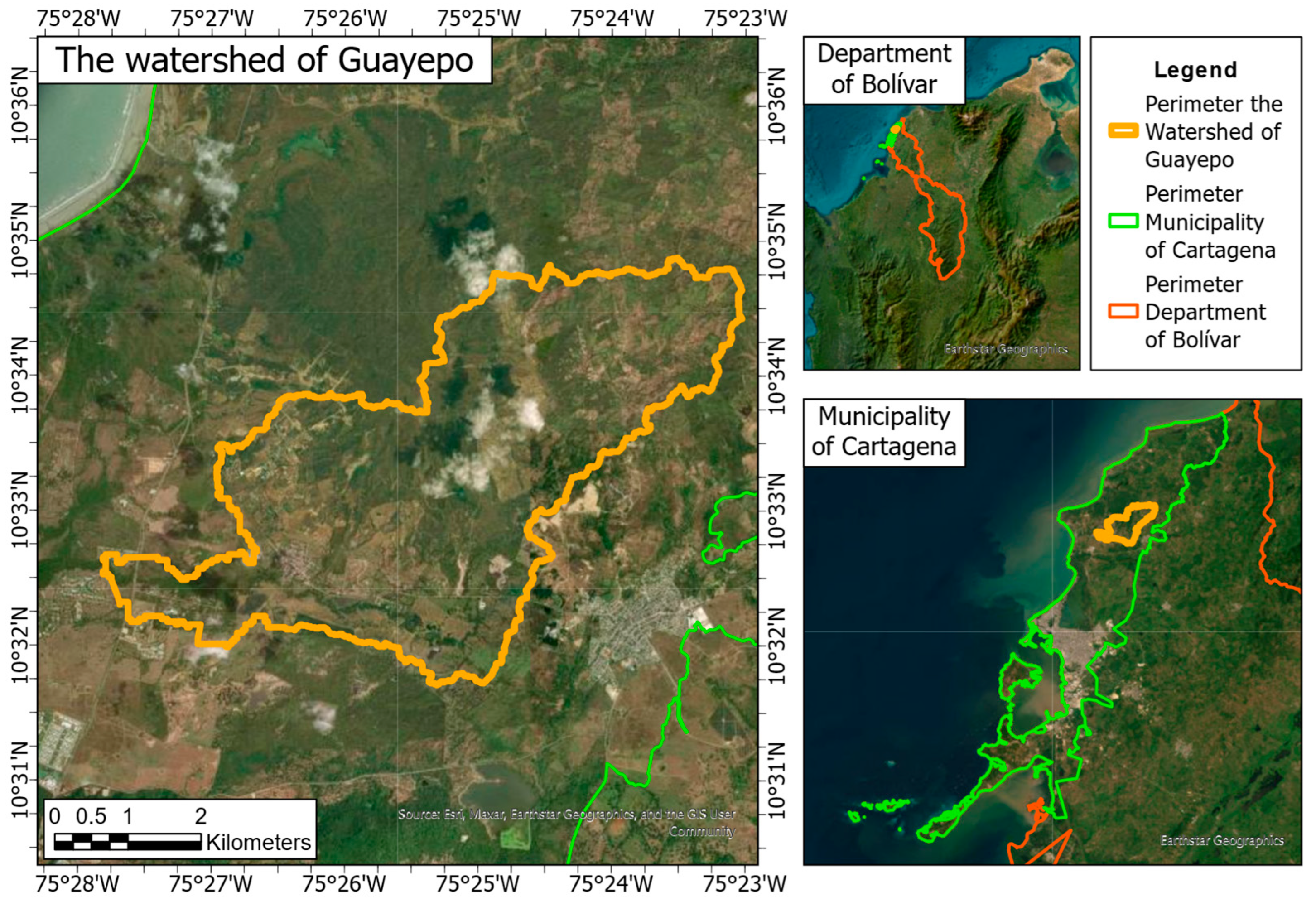
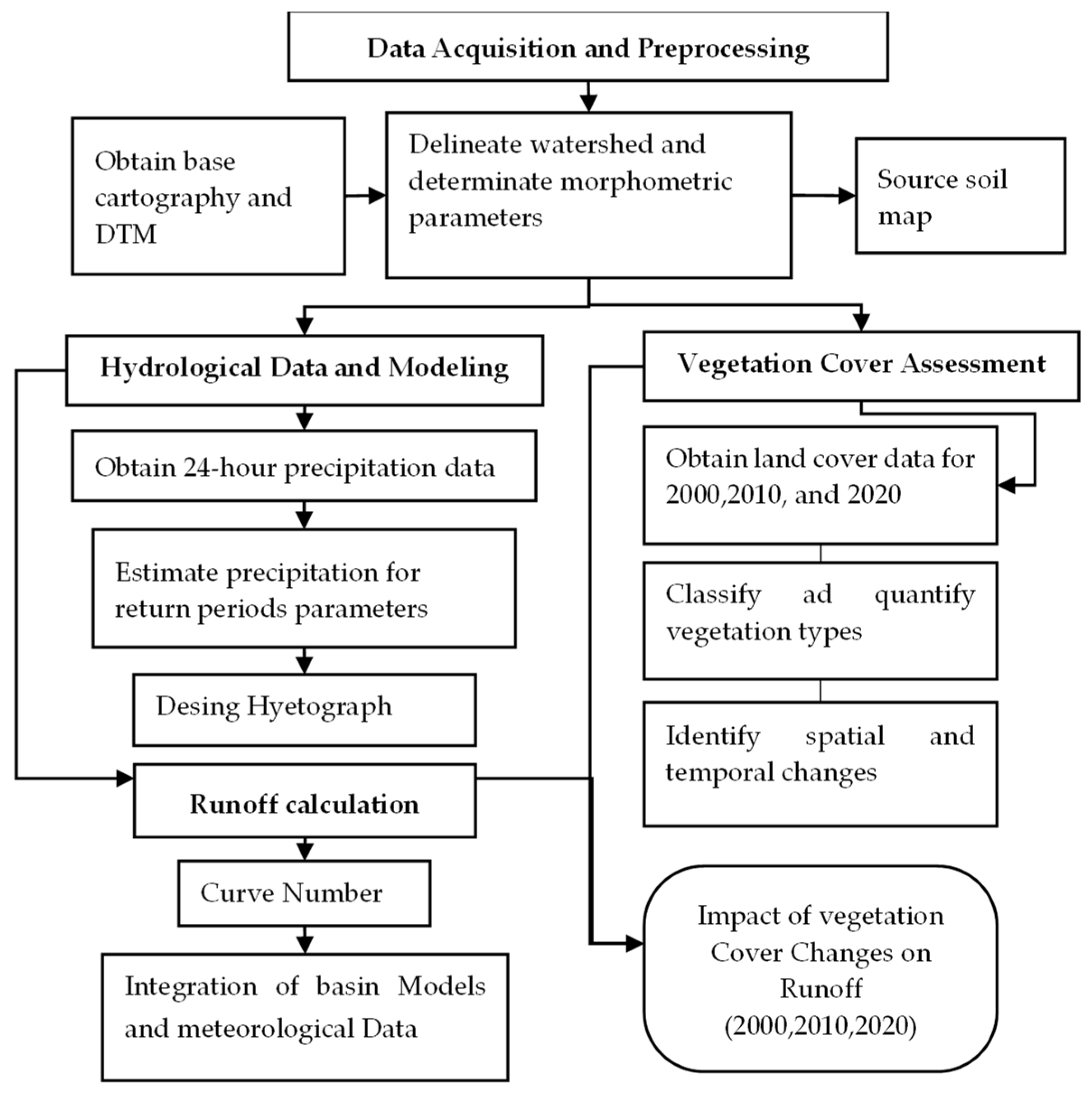
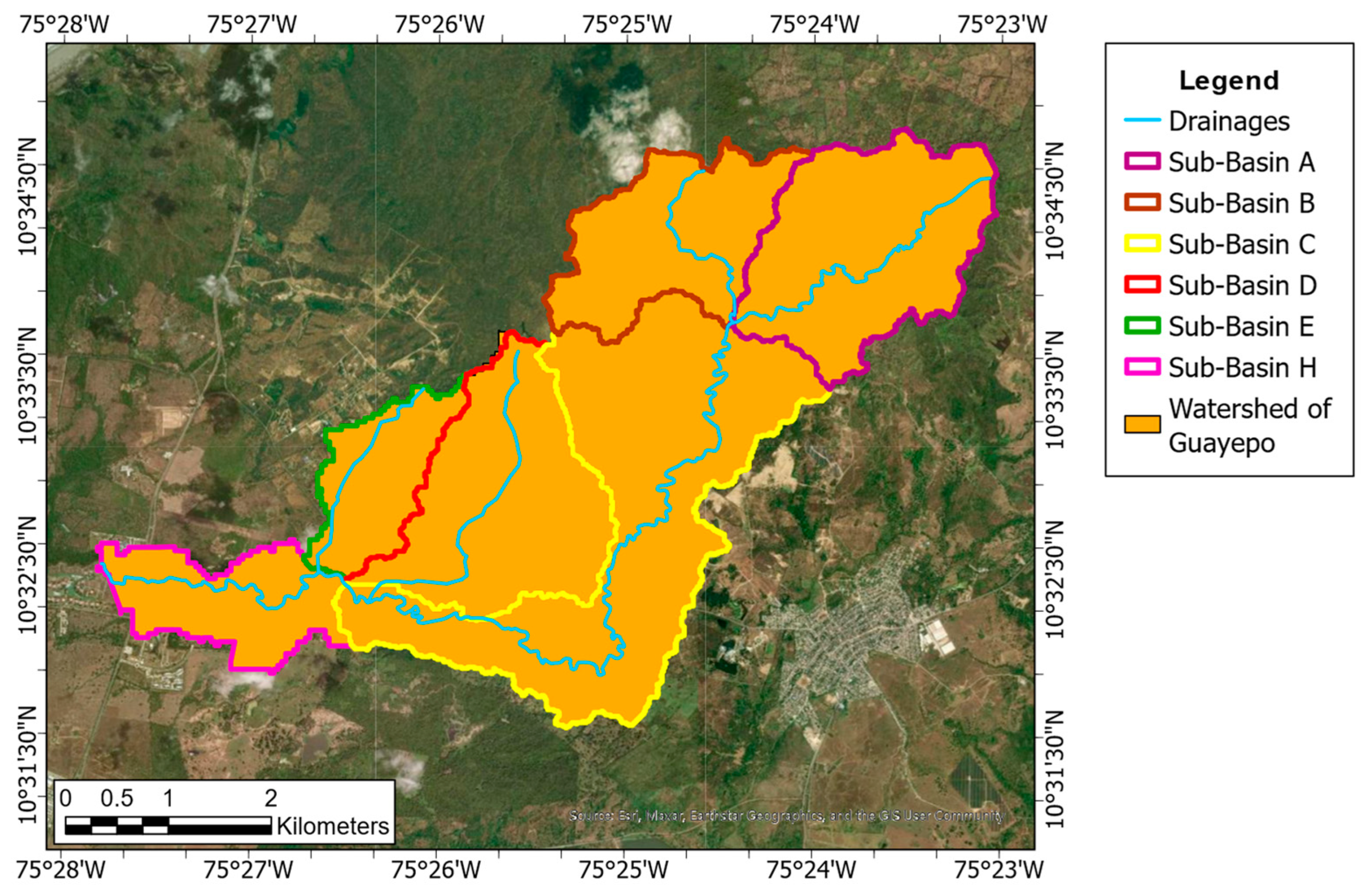
2.1. Data Acquisition and Preprocessing

The base cartography and digital terrain model (DTM) were obtained from the U.S. Geological Survey (USGS) geoportal (SRTM satellite) and the Agustin Codazzi Geographic Institute (IGAC). Land cover classification followed the CORINE land cover methodology adapted for Colombia at a 1:100,000 scale. The minimum mapping unit using Landsat imagery was set at 25 hectares for categories 2 to 5 and 5 hectares for category 1 of the national legend. For linear features such as roads and rivers, a minimum width of 50 m was applied, using the highest-resolution data available. This approach ensured consistent and reliable land cover identification for hydrological and environmental analysis.

These datasets facilitated the delineation of the watershed and the extraction of key morphometric parameters, including drainage area, perimeter, Gravelius index, form factor, concentration time, slope, and runoff coefficient. The compactness index ($K_c$) was determined using the perimeter and area of each sub-basin, indicating their shape and flood susceptibility. The form factor ($K_f$) was calculated to evaluate the elongation of the sub-basins and their potential for rapid runoff. Drainage density ($D_d$) was obtained by dividing the total stream length by the sub-basin area, providing insights into drainage efficiency. Sinuosity ($S)$ was measured as the ratio of the actual stream length to the straight-line distance, classifying streams as meandering or straight.

The time of concentration is one of the most important and challenging parameters to estimate in watershed studies due to the variety of available formulations. This study applied the most commonly used empirical methods, including the Kirpich formula, the California Culverts Practice, and the Bransby Williams approach [2,12,16]. The lag time, required as input data for the HEC-HMS model, was estimated as 60% of the average concentration time.

ArcGIS and Global Mapper were employed for the spatial analysis and characterisation of watershed morphology.

The soil map was sourced from the IGAC geoportal to determine soil profiles, classifications, and hydrological groups, complemented by previous soil studies conducted in the region. These datasets defined soil infiltration capacity and hydrological behaviour in runoff modelling.

2.2. Hydrological Data and Modelling

Maximum 24 h precipitation data from the Bayunca meteorological station, recorded between 1974 and 2019, were obtained from the IDEAM portal. These measured values served as the basis for estimating precipitation intensities associated with return periods of 25, 50, and 100 years. The Generalised Extreme Value (GEV) distribution was applied under stationary conditions to model these events, as it provided the best fit for the dataset. The used distribution is presented as follows:

$$f\left(x\right)={\displaystyle \frac{1}{\alpha }}{\left[1-{\displaystyle \frac{k}{\alpha }}(x-\mu )\right]}^{{\displaystyle \frac{1}{k}}-1}\exp \left\{-{\left[1-{\displaystyle \frac{k}{\alpha }}(x-\mu )\right]}^{{\displaystyle \frac{1}{k}}}\right\}$$

(1)

where $\mu$, $k$, and $\alpha$ are the distribution parameters.

Creating the IDF curves began with collecting historical maximum 24 h precipitation data from the Bayunca station (

Table A1. Annual 24 h maximum rainfall record.

Year	Precipitation (mm)	Year	Precipitation (mm)
1974	137	1997	94
1975	174	1998	62.5
1976	95	1999	106
1977	120	2000	32.5
1978	140	2001	112.2
1979	140	2002	90.3
1980	83	2003	80.5
1981	78.8	2004	122
1982	52.8	2005	106
1983	120	2006	138
1984	84	2007	122
1985	95.7	2008	108.5
1986	60.34	2009	81
1987	72.73	2010	109.3
1988	150	2011	75
1989	100	2012	105.1
1990	137	2013	56.1
1991	85.5	2014	132
1992	56.6	2015	50.5
1993	87.4	2016	121.8
1994	85	2017	50
1995	84	2018	85.4
1996	80	2019	127

), covering the period from 1974 to 2019, based on records from Diaz and Dávila [29].

Additionally, based on this precipitation series, intensity–duration–frequency (IDF) curves were derived using methodologies previously applied in hydrological analyses for the Cartagena de Indias airport station, as documented in several civil engineering undergraduate theses [30,31,32]. These methodologies were refined using precipitation–duration relationships proposed by Chang and Bolívar (1997) [33], allowing the adjustment of 24 h precipitation data to shorter durations required for hydrological modelling.

A correction was also applied to account for the recording method of 24 h rainfall data, which span from 7:00 a.m. to 7:00 a.m. the following day. Following the approach of Weiss Leonard [34] and Chulsang Yoo [35], a 13% increase was applied to the precipitation values to more accurately reflect continuous storm durations.

The watershed’s concentration time was first estimated to define the duration of the storm event. A representative rainfall duration of 9 h was selected, corresponding to approximately two to three times the concentration time, as recommended for hydrological modelling. Since storm temporal distribution directly affects the watershed’s hydrological response, a regional dimensionless rainfall distribution was used to construct the design hyetograph. To adjust the 24 h precipitation to a 9 h duration, a reduction factor of 0.94 was applied. This value was derived from the average of individual reduction factors calculated for each of the six historical storm events selected for the study. The reduction factor is calculated by dividing the total 24 h precipitation of the rainfall event chosen by the total precipitation during the selected 9 h period. This factor represents the percentage of the maximum 24 h rainfall that fell within the 9 h interval.

Storms recorded on 14 November 2020, 25 November 1997, 13 June 1971, 23 October 1978, 28 July 1980, and 3 October 1981 were analysed to establish the distribution of rainfall events. These storms were selected because they exhibited a representative rainfall duration of approximately 9 h, and in some of these periods, the occurrence of the La Niña phenomenon was observed.

The selected storms were chosen based on two criteria: (i) they presented rainfall durations close to 9 h, and (ii) some occurred during La Niña conditions, which are associated with high-intensity rainfall in the region. From these storms, exceedance percentages were derived. A 50% exceedance probability storm profile was selected for modelling purposes. The final hyetograph, constructed using the distributions of the six rainfalls adopted for the project, served as input for the HEC-HMS model to simulate runoff under different return periods.

2.3. Vegetation Cover Assessment

For land cover analysis, this study adopted a multi-temporal approach based on the CORINE land cover methodology adapted for Colombia. Land cover data were obtained from official sources at a 1:100,000 scale for 2000, 2010, and 2020 through the Colombian Environmental Information System (SIAC). These maps were processed in ArcGIS Pro3.4.0 to classify and quantify the vegetation types in the watershed for each reference year. This allowed for the accurate identification of spatial and temporal changes in vegetation cover and the calculation of percentage variations across the three decades.

2.4. Hydrological Modelling

Hydrological modelling in HEC-HMS was carried out using the curve number (CN) method to estimate peak flows, integrating four main components. First, the basin model was developed by importing a shapefile containing sub-basin boundaries and stream networks, defining elements such as sub-basin, reach, and sink. The curve number method was selected for losses, the curve number method unit hydrograph for runoff transformation, and the Muskingum–Cunge method for flood routing. Key input parameters included initial abstraction, CN values, lag times, reach length and slope, Manning’s roughness coefficient, and cross-sectional data.

Second, the time-series data component was configured by interpreting the results from the rain gauges, which record precipitation every 10 min in Colombia, and then aggregating the data into 20 min intervals. This approach was based on six representative nine-hour rainfall events. Third, the meteorological model was defined by linking the previously constructed hyetograph. Finally, the control specifications component was set up to define simulation intervals and output formats.

After running the model, outputs such as hydrographs, infiltration, and runoff tables were analysed and are presented in the Section 3.

3. Results

3.1. Data Processing and Preliminary Analysis

The watershed was delineated using the 30 m resolution Digital Elevation Model (DEM) from the United States Geological Survey’s geoportal and the contour lines obtained from the IGAC geoportal, as shown in Figure 3.

Next, the main watershed characteristics were calculated, as presented in

Table 1. Principal parameters of the watershed.

Parameters	Value
$\mathrm{Area}\left({\mathrm{k}\mathrm{m}}^2\right)$	21.06
$\mathrm{Perimeter}\left(\mathrm{k}\mathrm{m}\right)$	38.98
$\mathrm{Length}\mathrm{of}\mathrm{main}\mathrm{channel}\left(\mathrm{k}\mathrm{m}\right)$	22.9
$\mathrm{Maximum}\mathrm{axial}\mathrm{length}\left(\mathrm{k}\mathrm{m}\right)$	13.02

.

The Guayepo Basin watershed was considered for vegetation cover and runoff analysis and was divided into six sub-basins, as shown in Figure 4.

The morphometric parameters of the watershed, including compactness index, form factor, drainage density, and sinuosity, were calculated for all sub-basins to assess their hydrological characteristics, which are detailed in

Table 2. Calculated morphometric parameters in sub-basins A, B, C, D, E, and H.

Sub-Basin	Area ($\mathbf{k}{\mathbf{m}}^2$)	Length of the Channel (m)	Slope (m/m)	${\mathit{K}}_{\mathit{c}}$	${\mathit{K}}_{\mathit{f}}$	$\mathit{S}$
A	3.935	4067.21	0.00836	1.76	0.456	1.18
B	2.758	2283.19	0.01577	2.06	1.221	1.14
C	7.087	10,152.77	0.00217	2.61	0.265	1.52
D	3.840	3641.75	0.01922	1.83	0.443	1.03
E	1.552	2265.42	0.01501	1.89	0.375	1.09
H	1.885	3413.16	0.00234	1.94	0.350	1.25

.

Table 2 shows that Sub-basin C has the longest main channel, indicating an elongated shape based on its form factor. All sub-basins have a Gravelius Index (Kc) greater than 1, confirming their irregular shapes. Most sub-basins have a low form factor, suggesting they are elongated and less prone to flooding, except for Sub-basin B, which exceeds 1, indicating a higher tendency to concentrate runoff and generate large floods. Regarding sinuosity, Sub-basins A, B, D, and E have values below 1.25, meaning their main channels are straight, likely resulting in faster flow velocities. At the same time, the remaining sub-basins exhibit normal sinuosity.

Table 3. Concentration and lag times for sub-basins A, B, C, D, E, and H.

Sub-Basin	Tc Kirpich Minutes	Tc California Minutes	Tc Bransby Williams Minutes	Tc Mean Minutes	Lag Time Minutes
A	73.88	71.77	130.31	91.99	55.19
B	37.10	36.04	66.76	46.63	27.98
C	251.30	244.13	401.77	299.07	179.44
D	49.25	47.84	99.02	65.37	39.22
E	37.58	36.51	70.86	48.32	28.99
H	105.32	102.32	151.79	119.81	71.89

summarises the estimated values for the time of concentration and lag time obtained from the different methods.

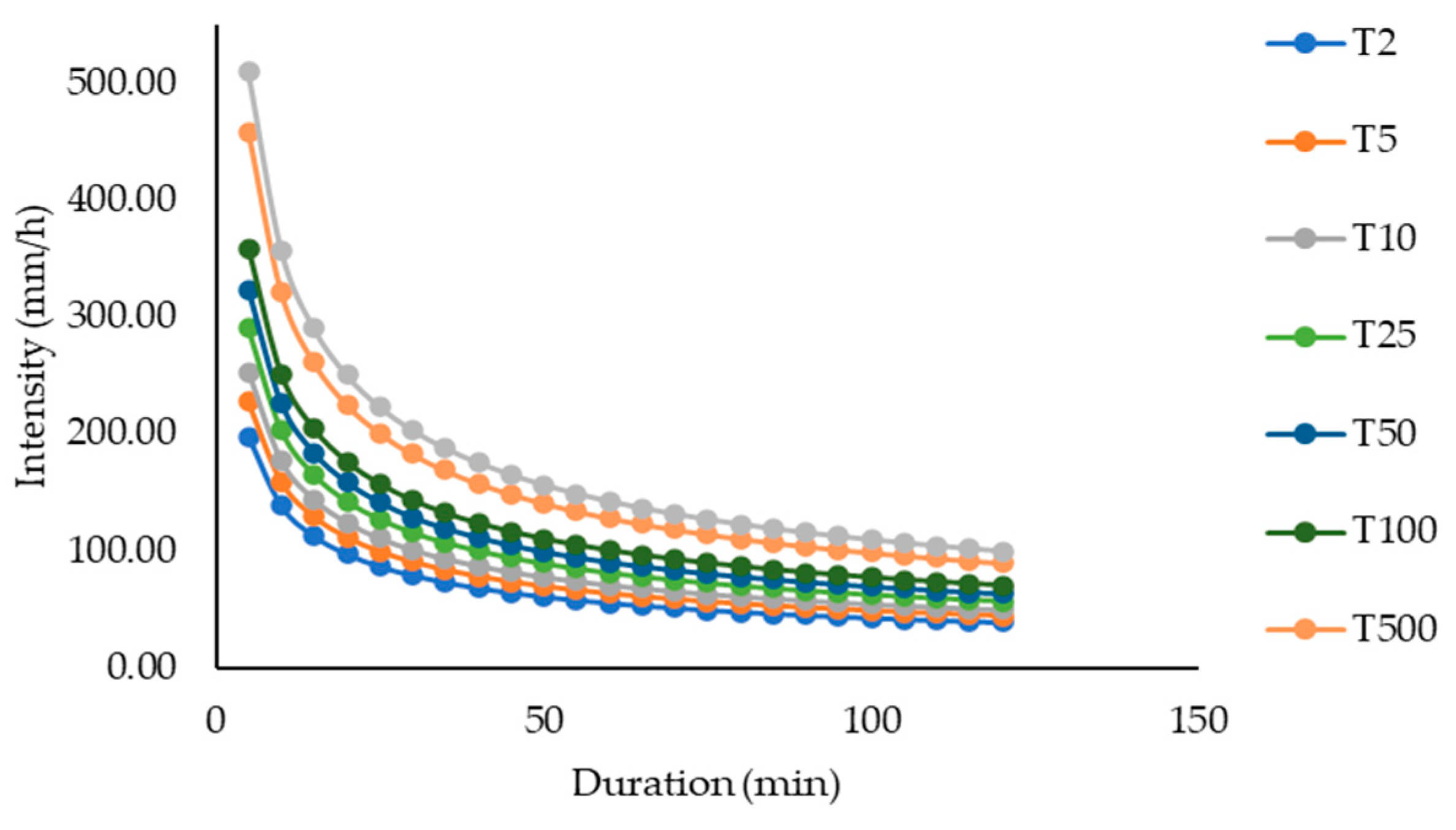
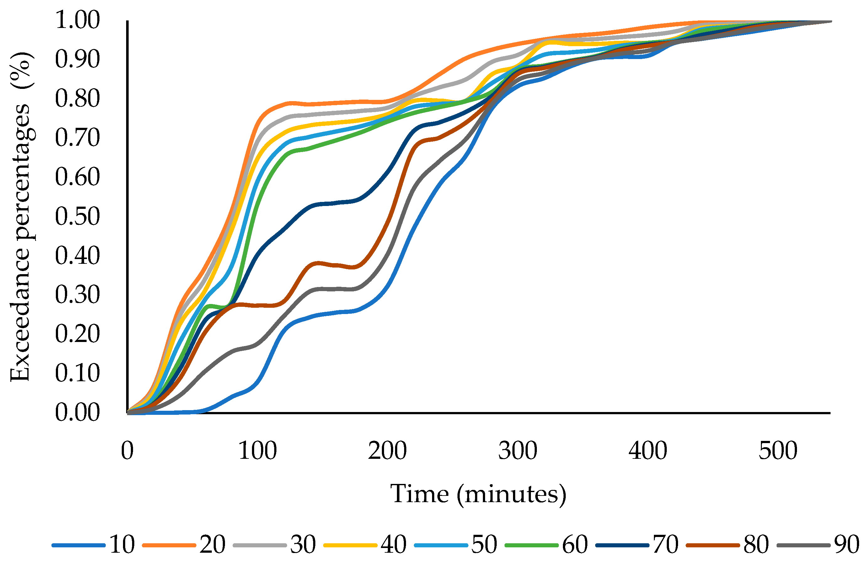
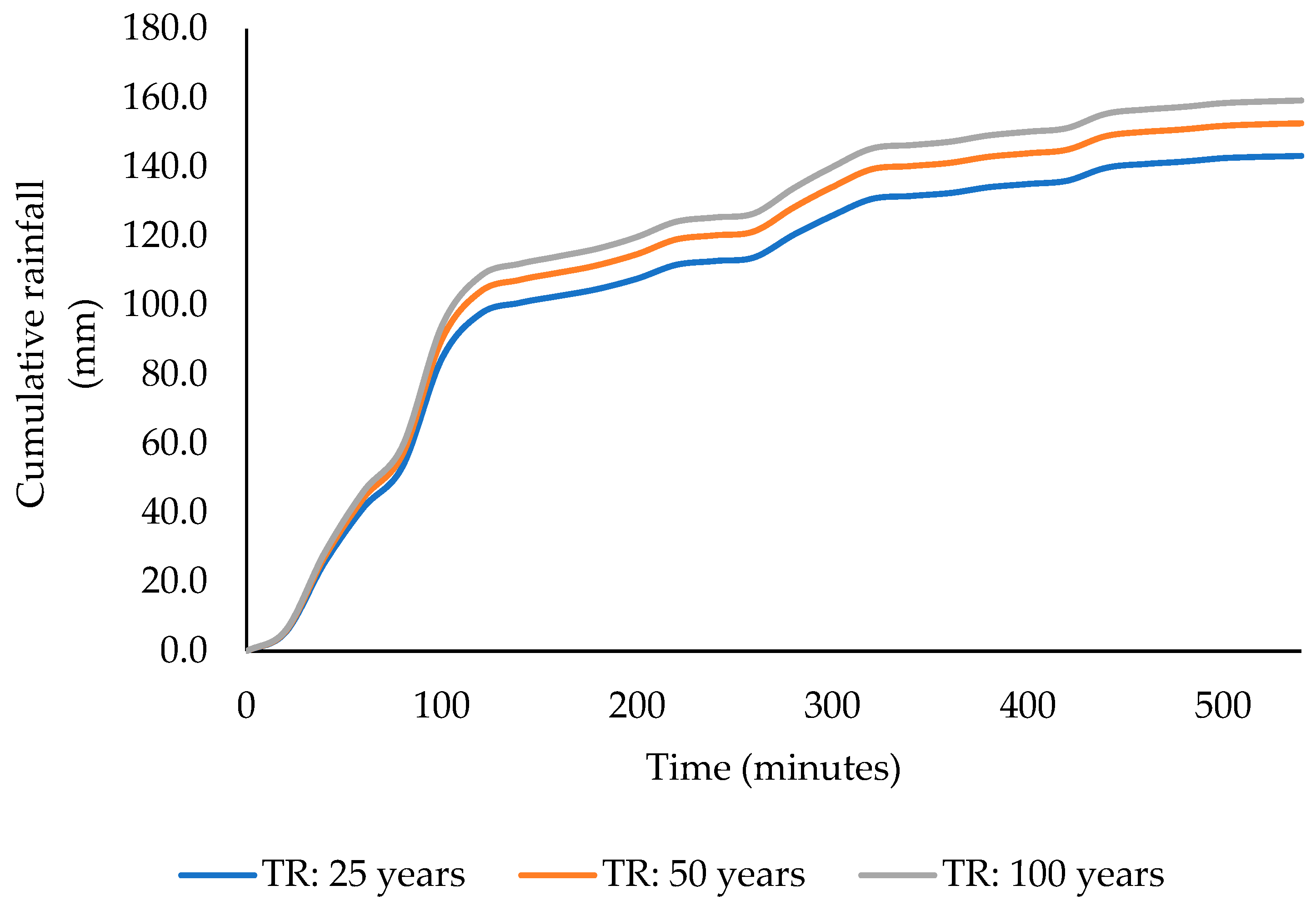
3.2. Precipitation Analysis and IDF Curves

Figure 5 presents the intensity–duration–frequency (IDF) curves for the Bayunca station, illustrating rainfall intensities and duration across different storm durations and return periods.

The annual maximum 24 h precipitation at the Bayunca station was estimated using the Generalised Extreme Value (GEV) probability distribution, as it provided the best fit according to the Chi-square test, with a value of 5.26, based on the maximum likelihood method for parameter estimation. The results for the mean and the 95% confidence intervals of the maximum daily precipitation are presented in

Table 4. Probabilistic adjustment of maximum 24 h precipitation using the Gumbel probability distribution, Bayunca Station.

Tr (Years)	Pmax-24 h (mm)
	Mean *	Confidence Intervals **
100	169	148–190
50	162	144–179
25	152	138–167
20	149	135–163
10	138	126–150
5	123	113–134
3	110	99.9–120
2	96.4	86.9–106

* Values used for hydrological analysis. ** The results are presented with 95% confidence intervals to indicate the range of uncertainty.

. The Chi-square values for the Gumbel distribution (maximum likelihood method) and the Log-Pearson Type III distribution (method of moments) were 13.09 and 5.65, respectively.

For this analysis, a rainfall duration of 9 h was considered for modelling, based on a range between 2 and 3 times the basin’s concentration time.

Table A2. Cumulative rainfall from design storms.

	1	2	3	4	5	6
P Max 24 h (mm)	142.55	101.7	108.5	65.1	135.3	72.4
Factor Reduction Time	0.89	0.94	0.92	0.92	0.99	0.99
t (min)	14-nov-20	25-nov-97	13-jun-71	23-oct-78	28-jul-80	3-oct-81
0	0.00	0.00	0.00	0.00	0.00	0.00
20	0.09	2.00	5.10	4.00	3.40	10.20
40	0.19	8.30	27.00	8.00	30.10	19.10
60	0.93	30.00	37.20	12.40	52.60	19.10
80	5.15	57.30	46.50	16.90	69.00	19.40
100	10.11	79.30	64.80	31.90	98.90	19.60
120	26.51	84.50	71.20	39.00	105.60	20.30
140	31.03	87.50	73.20	40.40	105.70	26.80
160	32.54	88.10	73.90	41.60	106.20	26.90
180	33.90	88.30	74.60	42.90	106.60	27.20
200	41.22	89.20	76.10	44.50	106.80	34.80
220	59.70	89.90	82.00	45.80	106.90	48.10
240	74.13	89.90	86.30	46.70	107.00	50.20
260	83.31	89.90	90.30	47.60	107.00	52.90
280	98.66	89.90	92.50	49.00	107.10	61.70
300	109.87	89.90	94.00	49.90	118.90	62.50
320	111.80	89.90	96.00	51.10	127.90	63.30
340	113.73	89.90	97.10	52.90	129.10	64.20
360	115.66	89.90	97.30	54.20	129.80	64.60
380	117.59	90.20	98.40	55.70	130.80	64.90
400	119.00	90.20	98.70	56.50	132.10	65.10
420	120.14	90.50	98.90	57.10	133.30	67.40
440	121.28	91.10	99.40	58.20	133.80	70.10
460	122.42	92.40	99.70	58.80	134.00	70.50
480	123.59	93.90	99.90	59.20	134.20	70.70
500	124.92	95.20	99.90	59.60	134.30	70.80
520	126.25	95.40	99.90	59.80	134.40	71.00
540	127.16	95.60	99.90	59.90	134.40	71.50

presents the accumulated precipitation for each storm at 20 min intervals. Based on these storms, exceedance percentages were calculated, as shown in Figure 6.

For the analysis, a rainfall event with an exceedance probability of 50% or greater was considered.

Using a dimensionless temporal rainfall distribution allowed for the development of a storm hyetograph design based on the pluviograph records of the six storms analysed in this study (see Table A2).

Based on the obtained results, the design rainfall distributions for various return periods were developed, as presented in Figure 7; the detailed results can be seen in

Table A3. Design rainfall distributions for various return periods.

Return Periods
t (min)	5	10	20	25	50	100
0	0.0	0.0	0.0	0.0	0.0	0.0
20	4.4	5.0	5.4	5.5	5.8	6.1
40	20.7	23.2	25.1	25.6	27.3	28.5
60	33.7	37.8	40.8	41.6	44.3	46.3
80	43.3	48.6	52.5	53.5	57.1	59.5
100	68.5	76.8	82.9	84.6	90.2	94.1
120	79.0	88.7	95.7	97.7	104.1	108.6
140	81.5	91.5	98.8	100.8	107.4	112.0
160	83.1	93.3	100.7	102.7	109.5	114.2
180	84.8	95.1	102.7	104.8	111.7	116.5
200	87.2	97.8	105.6	107.8	114.8	119.8
220	90.4	101.4	109.5	111.7	119.1	124.2
240	91.3	102.5	110.6	112.8	120.3	125.5
260	92.2	103.4	111.7	113.9	121.4	126.7
280	97.4	109.3	118.0	120.4	128.3	133.8
300	101.9	114.4	123.5	126.0	134.2	140.0
320	105.8	118.7	128.2	130.7	139.3	145.4
340	106.5	119.5	129.1	131.6	140.3	146.4
360	107.2	120.3	129.9	132.5	141.2	147.3
380	108.6	121.8	131.5	134.2	143.0	149.2
400	109.3	122.7	132.5	135.1	144.0	150.2
420	110.1	123.5	133.4	136.1	145.0	151.3
440	113.1	126.9	137.0	139.8	149.0	155.4
460	114.0	127.9	138.1	140.9	150.2	156.7
480	114.6	128.6	138.8	141.6	150.9	157.4
500	115.4	129.4	139.8	142.6	152.0	158.5
520	115.7	129.8	140.1	143.0	152.4	158.9
540	115.9	130.0	140.4	143.2	152.7	159.2

.

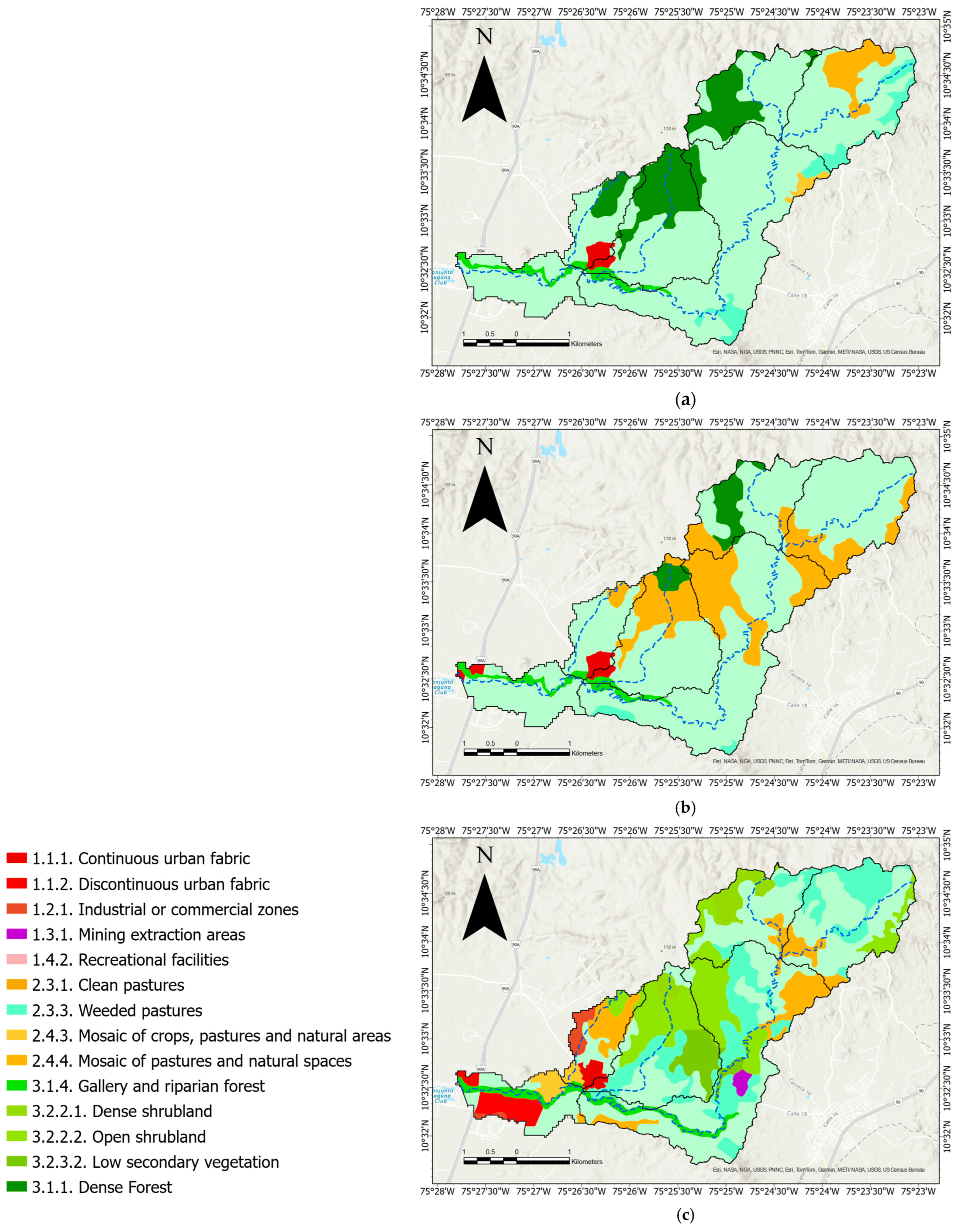
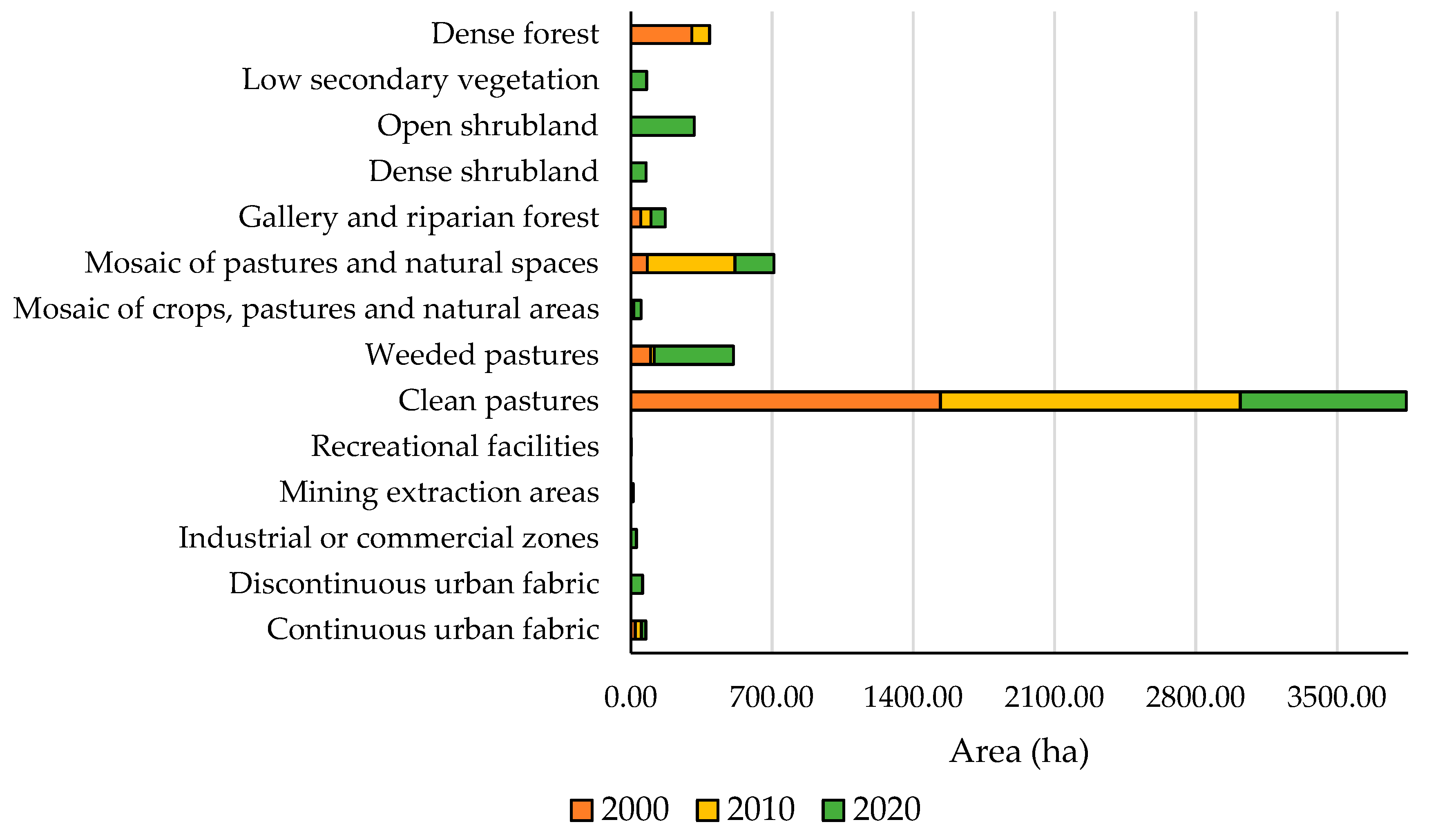
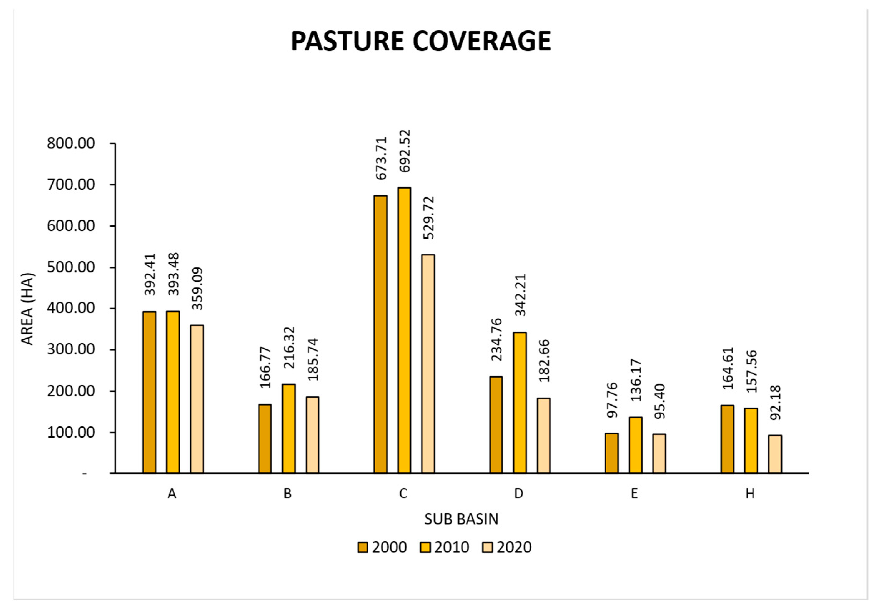
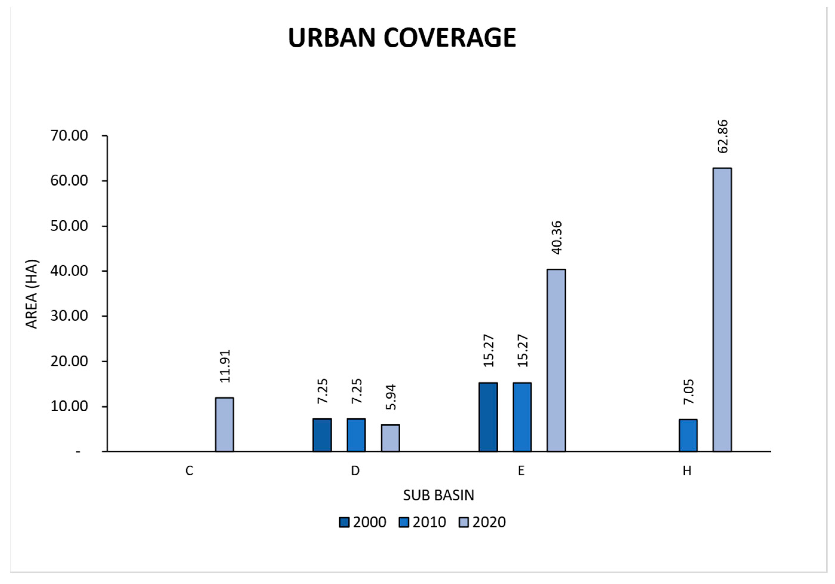
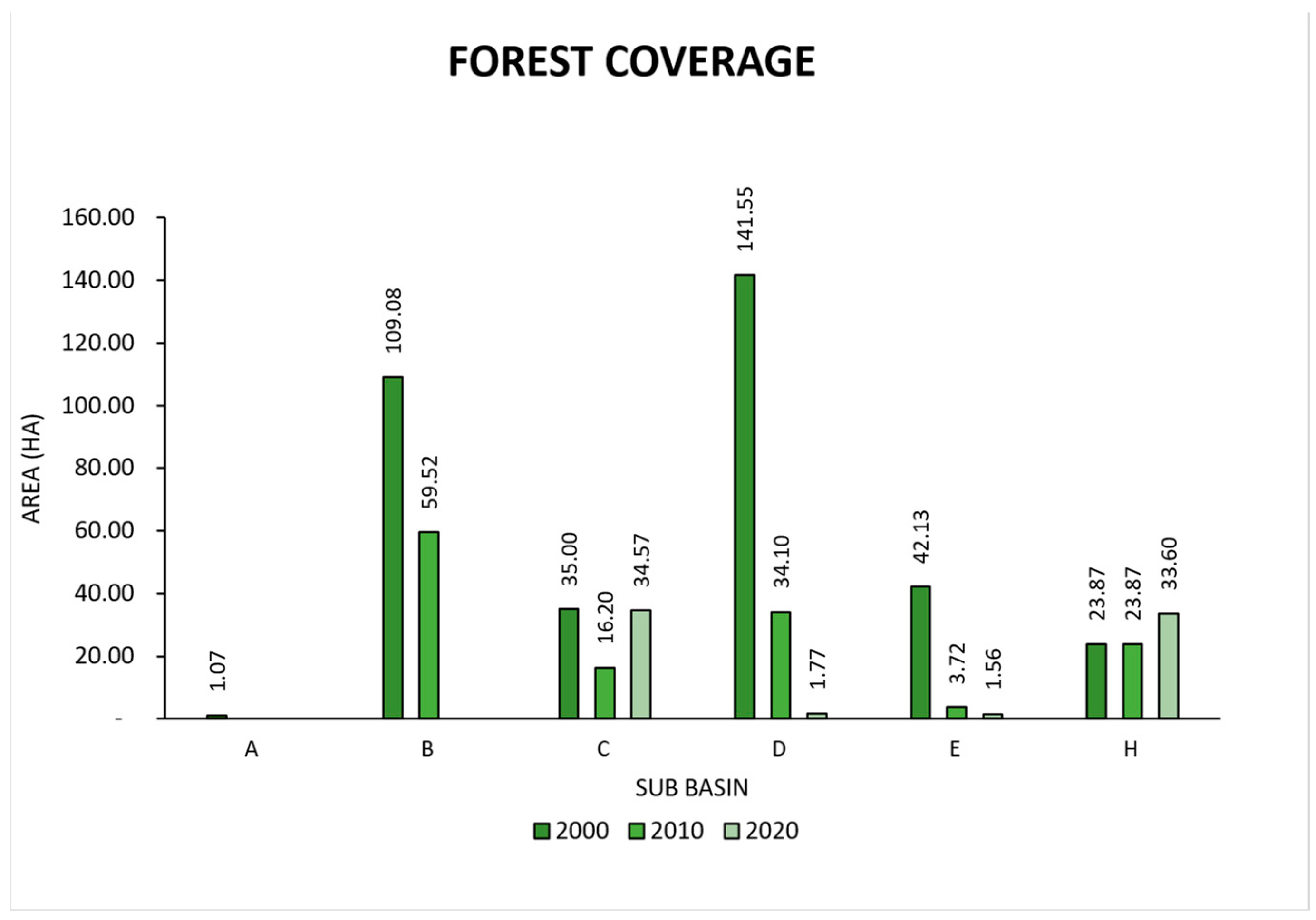
3.3. Vegetation Cover Change Assessment

This study conducted a multitemporal analysis of land cover changes in the area using the CORINE land cover methodology adapted for Colombia and Google’s digitalisation tool. The results for 2000, 2010, and 2019 are presented in Figure 8.

The areas (%) of each cover were determined for each year, and the data were plotted in the table to analyse the variations found between each study period.

Table 5. Change in cover in 2000, 2010, and 2020.

	Area (%)
Coverage	2000	2010	2020
Continuous urban fabric	1.07	1.40	1.06
Discontinuous urban fabric	0.00	0.00	2.77
Industrial or commercial zones	0.00	0.00	1.33
Mining extraction areas	0.00	0.00	0.57
Recreational facilities	0.00	0.00	0.01
Clean pastures	72.90	70.56	39.07
Weeded pastures	4.68	0.85	18.65
Mosaic of crops, pastures, and natural areas	0.72	0.00	1.70
Mosaic of pastures and natural spaces	3.88	20.65	9.15
Gallery and riparian forest	2.37	0.00	3.39
Dense shrubland	0.00	0.00	3.61
Open shrubland	0.00	0.00	14.93
Low secondary vegetation	0.00	0.00	3.76
Dense forest	14.38	4.16	0.00
Gallery and riparian forest	0.00	2.37	0.00

reveals land cover transformations in the study area over the 20 years from 2000 to 2020, reflecting a shift from predominantly rural and natural landscapes toward more urbanised and fragmented systems.

In 2000, clean pastures largely dominated the landscape, covering 72.90% of the area, followed by dense forest (14.38%) and riparian forest (2.37%). Urban coverage was minimal at just 1.07%, which aligns with the Cartagena Territorial Ordering Plan (POT) of 2001, which designated the area primarily for agriculture and livestock.

By 2010, clean pastures remained dominant (70.56%), but early signs of transformation were evident. Dense forest had declined to 4.16%—a 71% reduction. Urban areas expanded moderately, with continuous urban fabric increasing by 31%, and industrial/commercial areas appeared for the first time (1.33%). Meanwhile, a rise in mosaics of pastures and natural spaces (20.65%) pointed to early fragmentation of the landscape and a shift toward mixed-use rural systems.

The most drastic changes occurred by 2020, marking a turning point in the region’s ecological structure. Dense forest cover was lost entirely, and riparian zones had vanished, totalling a forest loss of over 268 hectares. Urbanisation intensified, with the emergence of discontinuous urban fabric (2.77%), and total urban land uses (continuous and discontinuous urban fabric, industrial or commercial zones, and mining extraction areas) rose to 5.73%—a 435% increase since 2000 (1.07%). Simultaneously, clean pastures declined to 39.07%, while improved pastures grew to 18.65%, indicating a transition to more intensive livestock systems. Mosaic landscapes continued expanding, reinforcing a shift away from natural ecosystems toward human-dominated land uses.

Additionally, new vegetation types emerged between 2010 and 2020, such as dense shrubland (3.61%), open shrubland (14.93%), and low secondary vegetation (3.76%), likely reflecting early regeneration or degradation responses. The appearance of mining zones (0.57%) and recreational spaces (0.01%) further highlighted a growing trend toward land transformation for urban, industrial, and infrastructural development.

Similarly, a detailed spatial analysis was conducted to identify the area covered by each land use category.

Figure 9 reveals that in 2000, the landscape was dominated mainly by clean pastures, occupying 1534.78 hectares or 72.91% of the total basin area. This was followed by dense forest, 302.81 ha (14.37%), and riparian or gallery forest, 49.89 ha (2.37%). Urban land use was minimal, with continuous urban fabric accounting for just 1.07% and no presence of industrial, commercial, or mining activities.

By 2010, clean pastures remained dominant, slightly decreasing to 1485.53 ha (70.51%). However, signs of transformation began to emerge. Dense forest shrank to 87.52 ha (4.15%), marking a 71% loss, while riparian forest remained unchanged. Urbanisation showed moderate growth: continuous urban fabric rose to 29.57 ha, a 31% increase, and industrial/commercial zones appeared for the first time, covering 28.05 ha (1.33%). Most notably, the mosaic of pastures and natural areas expanded to 434.75 ha (20.64%), signalling early fragmentation of the landscape and a shift toward mixed rural uses.

By 2020, the most drastic changes became evident. Dense forest was utterly lost, and riparian forest also disappeared, resulting in a total forest (gallery and riparian forest and dense forest) loss exceeding 352 hectares, equivalent to 16.7% of the basin. Urbanisation intensified with discontinuous urban fabric (58.48 ha or 2.78%). In contrast, total urban and related land uses (continuous, discontinuous, industrial, mining, and recreational) reached 98.57 ha or 4.68%, marking a 337% increase from 2000.

Simultaneously, clean pastures declined to 823.24 ha (39.08%), while weeded or improved pastures increased significantly to 392.92 ha (18.65%), reflecting a shift toward more intensive livestock systems. Mosaic landscapes continued to grow, with pasture–natural mosaics covering 192.72 ha (9.15%) and a mosaic of crops, pastures, and natural areas reappearing with 35.91 ha (1.71%)—both reinforcing the transition away from pristine ecosystems.

Analysing which areas have experienced the most significant changes is essential to better understanding land cover variations. Therefore, Figure 10, Figure 11 and Figure 12 present the analysis of land cover variation in each sub-basin over the years we studied.

Figure 10 shows notable spatial variability in pasture coverage across the sub-basins during the study period (2000–2020). Sub-basin C consistently held the largest pasture area, peaking in 2010 (691.52 ha), but it experienced a marked decline of approximately 23% by 2020 (529.72 ha), suggesting a potential land use shift toward urbanisation, natural regeneration, or abandonment. Similarly, Sub-basin H recorded the most significant relative decrease, with a 37% loss in pasture area over two decades, likely linked to urban expansion or ecological restoration. Sub-basin E also followed a declining trend, though less pronounced, hinting at gradual transformation processes.

In contrast, Sub-basin D exhibited a moderate reduction in pasture coverage, decreasing from 342.21 ha in 2010 to 234.76 ha in 2020, which may reflect land conversion to other uses or natural vegetation recovery. Sub-basins A and B exhibited excellent stability, with A maintaining nearly constant values and B showing a slight upward trend. These variations reflect differing land management dynamics across the sub-basins, highlighting both pressures from urban growth and efforts to preserve or restore rural land uses.

Figure 11 reveals significant spatial and temporal variability in urban land cover across Sub-basins C, D, E, and H between 2000 and 2020. Sub-basin H experienced the most dramatic increase, from 7.05 ha in 2000 to 62.86 ha in 2020. This sharp rise suggests intense urbanisation pressure, likely driven by population growth, infrastructure development, or changes in land use planning. Similarly, Sub-basin E showed a notable shift, maintaining a stable urban area of 15.27 ha from 2000 to 2010 before more than doubling to 40.36 ha by 2020, indicating recent urban expansion or settlement consolidation.

In contrast, Sub-basin D displayed a slight decline in urban area, decreasing from 7.25 ha in 2000 and 2010 to 5.94 ha in 2020, possibly reflecting urban retreat, land use reclassification, or abandonment. Meanwhile, Sub-basin C—initially with no recorded urban cover—saw a moderate increase to 11.91 ha in 2020, suggesting emerging urban development. These divergent patterns highlight the varied dynamics of urban growth, emphasising the need for adaptive and spatially sensitive land use planning.

Figure 12 illustrates distinct patterns in forest coverage across Sub-basins A through H from 2000 to 2020, revealing significant losses and relative stability areas. Sub-basin D experienced the most dramatic deforestation, decreasing from 141.55 ha in 2000 to just 1.77 ha in 2020—a loss of nearly 99%, likely due to urban expansion, agricultural development, or land degradation. Similarly, Sub-basin B saw a marked decline, from 109.08 ha in 2000 to 59.52 ha in 2020, underscoring sustained pressure on forested areas over two decades.

In contrast, Sub-basin C maintained relatively stable forest coverage, with only a slight decrease from 35 ha in 2000 to 34.57 ha in 2020, suggesting effective conservation or limited development pressure. Sub-basin H also showed minimal change, fluctuating between 23.87 ha and 39.60 ha. Meanwhile, with very low forest cover initially, Sub-basins A and E experienced minor increases by 2020, possibly due to natural regeneration or reforestation efforts. These contrasting trends highlight critical areas for targeted forest management and reflect the varied impact of land use dynamics across the watershed.

3.4. Hydrological Simulation Using the HEC-HMS Model

One of the input parameters for modelling in HEC-HMS software is the curve number, which is used to apply the curve number method for abstraction. Estimating this parameter requires knowledge of the soil hydrologic group.

Since all identified profiles have clayey or silty clay textures, the hydrologic group was classified as D. With this classification, curve numbers were selected from tables provided by the SCS curve number method, available in the HEC-HMS Technical Reference Manual.

The hydrological soil group for the basin was determined using the relationship established by Rawls et al. (1983) [36,37] based on the depth of the soil layers, the soil in each profile belongs to Group D. This means the soil has a loam–clay, silt–clay–loam, sand–clay, or silt–clay texture with an average permeability characteristic for semi-permeable soils.

All curve numbers refer to antecedent moisture condition (AMC) II, representing normal soil moisture. Curve numbers for dry antecedent moisture (AMC I) and fully saturated antecedent moisture, the most critical condition (AMC III), were also considered.

Table 6. Curve number of Sub-basins A, B, C, D, E and F for each antecedent moisture condition.

	The Year 2000			The Year 2010			The Year 2020
Sub-Basins	CN (I)	CN (II)	CN (III)	CN (I)	CN (II)	CN (III)	CN (I)	CN (II)	CN (III)
A	64.48	83.10	91.87	63.04	82.13	91.36	65.33	83.66	92.17
B	58.36	78.81	89.54	60.87	80.62	90.54	63.51	82.44	91.52
C	60.92	80.65	90.55	63.43	82.39	91.50	65.85	84.00	92.35
D	58.94	79.23	89.77	63.78	82.63	91.62	66.94	84.71	92.72
E	61.35	80.96	90.72	64.00	82.78	91.70	73.02	88.45	94.63
H	59.47	79.62	89.99	60.41	80.29	90.36	68.49	85.70	93.23

presents the curve number values for each antecedent moisture condition.

Table 7. Initial abstraction of Sub-basins A, B, C, D, E and F for each antecedent moisture condition.

	The Year 2000			The Year 2010			The Year 2020
Sub-Basins	CN (I)	CN (II)	CN (III)	CN (I)	CN (II)	CN (III)	CN (I)	CN (II)	CN (III)
A	27.98	10.33	4.49	29.78	11.06	4.81	26.96	9.93	4.32
B	36.24	13.66	5.94	32.65	12.21	5.31	29.19	10.82	4.70
C	32.59	12.19	5.30	29.29	10.86	4.72	26.35	9.68	4.21
D	35.40	13.31	5.79	28.84	10.68	4.64	25.08	9.17	3.99
E	32.00	11.95	5.20	28.57	10.57	4.60	18.77	6.63	2.88
H	34.62	13.00	5.65	33.29	12.47	5.42	23.37	8.48	3.69

presents the initial abstraction values used in this research, considering 20% of the maximum potential retention.

Subsequently, modelling was performed for each study year (2000, 2010, and 2020) and each corresponding return period (25, 50, and 100 years). The curve number parameter was determined for antecedent moisture conditions AMC I and AMC II to calculate runoff flows in HEC-HMS software (see

Table 8. Peak flow for various return periods and antecedent moisture conditions.

Year	Return Period (Years)	Flow (m3/s)
		AMC I	AMC II
2000	25	40.20	80.70
	50	46.00	89.20
	100	49.60	94.80
2010	25	43.30	83.20
	50	49.00	91.60
	100	52.60	97.20
2020	25	49.20	93.40
	50	54.50	101.70
	100	58.90	108.80

).

Data on sub-basin areas were entered, the loss method was selected, and the curve numbers and initial abstraction were added. Then, the transformation method was chosen, and the lag times were provided to the model.

The analysis of runoff flow variations calculated with the HEC-HMS model under different antecedent moisture conditions (AMCs) and return periods reveals significant hydrological changes in the study area between 2000, 2010, and 2020. These variations reflect the progressive transformation of land cover and its influence on the basin’s hydrological response, especially as vegetation cover was reduced and impervious surfaces expanded.

Under AMC I conditions, which correspond to dry antecedent moisture, the basin exhibits a marked increase in flow across all return periods. For a 25-year return period, flow increased from 40.20 m³/s in 2000 to 49.20 m³/s in 2020, representing an increment of 22.4% in the modelled peak. For 50- and 100-year return periods, flows rose from 46.00 to 54.50 m³/s and from 49.60 to 58.90 m³/s, with respective increases of 18.5% and 18.8%. These trends suggest that even under dry soil conditions, the basin’s capacity to absorb rainfall has diminished over time, likely due to reduced natural vegetation and the increase in compacted or urbanised land covers. Such land transformation limits infiltration and enhances surface runoff, making the watershed more hydrologically reactive.

Similarly, runoff flows also increased under AMC II conditions, which represent intermediate soil moisture levels, though with moderate variations. In the year 2000, for a 25-year return period, the flow was 80.70 m³/s, increasing to 93.40 m³/s by 2020, representing a 15.7% rise. The increases for the 50- and 100-year return periods were 14.0% and 14.8%, respectively, reaching 101.70 m³/s and 108.80 m³/s. These increases indicate that, although the soil was already moist, the reduction in infiltration capacity and loss of forest cover continued to influence runoff generation. Notably, even in conditions with higher antecedent moisture, the transformation of the landscape exacerbates peak flows, increasing the risks of flash floods and soil erosion.

4. Discussion

The results obtained from the HEC-HMS model highlight notable variations in runoff flows across the years 2000, 2010, and 2020, driven by changes in land cover and antecedent moisture conditions (AMCs). These findings underscore the increasing hydrological sensitivity of the watershed, as the reduction in vegetation and expansion of impervious surfaces have progressively diminished its infiltration capacity, resulting in higher peak discharges even under dry conditions (AMC I).

Given these trends, it becomes evident that instrumenting the watershed is essential to accurately measure surface runoff and key parameters needed for flood routing using the Muskingum–Cunge method. Such instrumentation would enable real-time data collection and facilitate the calibration of the curve number (CN) model in HEC-HMS, ultimately enhancing the reliability of the simulated hydrographs and supporting better flood risk management in the area.

It is of utmost importance that decision-makers invest in Cartagena de Indias, which currently lacks such infrastructure. These efforts are essential for enhancing the quantification of flood hazards and, consequently, for reducing flood risk in the area. The selection of methods and parameters was based on previous studies widely recognised and accepted in Colombia [12,25].

The increase in flow rates between 2000 and 2020, observed across all return periods, confirms a general trend of rising water availability in the study area. Events with a 50-year return period show a more notable increase in the last decade (2010–2019), while events with 25-year and 100-year return periods exhibit a more significant rise in the first decade (2000–2010).

Although the increases in estimated peak flows are moderate, the upward trend is steady, implying that land use or climate changes have yet to produce drastic impacts but are contributing to gradual shifts. These results highlight the importance of long-term monitoring, as the gradual rise in flow rates could have significant implications for the region’s water resource management and infrastructure.

Results indicate that between 2000 and 2020, vegetation cover significantly declined. Dense forests, for instance, disappeared entirely, dropping from 14.38% of the basin area in 2000 to 0% by 2020, representing a loss of over 5.4 km². This was compounded by the disappearance of gallery and riparian forests by 2020, which had covered 2.37% of the area in 2010. In contrast, new land cover types emerged, such as discontinuous urban fabric and open shrubland, which reached 2.77% and 14.93%, respectively, in 2020. Additionally, weeded pastures expanded dramatically from 0.85% to 18.65% between 2010 and 2020. These changes reveal an accelerated process of landscape transformation, primarily driven by urban expansion and extensive livestock farming, highlighting the urgent need for integrated watershed management strategies that support ecological restoration and water sustainability.

Riparian vegetation is essential for maintaining a healthy river ecological system, improving carbon sequestration rates; controlling temperature, moisture, sediment, and nutrient pollution entering the river; and more. Vegetation in watersheds has historically transformed from natural forests to cultivation and urbanisation. Human intervention is an essential factor affecting vegetation conditions in riparian zones. In regions where river channels have primarily gentle slopes and extensive floodplains, riparian vegetation reduces the amplitude and peak of flood hydrographs [38].

Given climate change scenarios, proper management of water resources is essential to achieve sustainable development and avoid crises due to limitations in water availability, especially for human consumption. If the stressors that gave rise to a degraded ecosystem are removed, natural regeneration will begin with community support, given that community participation is significant throughout the restoration process [38,39,40].

For ecological restoration, it is necessary to review ecological descriptions of natural vegetation, species lists, and their composition and dynamics before disturbance, using primary data collection, aerial photographs, satellite images, etc., which can be complemented by studies already conducted by government institutions. Evaluate the current state of the ecosystem to be restored; this requires locating remnants or patches of the original ecosystem in terms of the number of patches, size, shape, and connectivity. Also, consider the types of land uses where the relics are found, the location of seed-dispersing fauna, regional climate conditions regarding rainfall distribution, dry season length, daily temperature fluctuations, and other climatic factors. In the Guayepo study area, it is essential to restore the tropical dry forest zone with its main species (Gliricidia sepium, Ceiba pentandra, Tabebuia rosea, Tabebuia chrysantha, Aspidosperma dugandii, Crescentia cujete, Juglans neotropica, Manilkara zapota, Chrysophyllum cainito, Melicoccus bijugatus, etc.) by seeking to transform pasture and crop areas into natural spaces, especially in the upper and middle-upper parts of the basin. This requires constructing and maintaining nurseries to propagate and grow native plants. If necessary, establish experimental plots for species combinations and the design of specific treatments. Above all, secure the support of the local community in these processes. Finally, the cost-effectiveness of different restoration techniques should be evaluated based on available resources [41].

5. Conclusions

The Guayepo Stream basin, covering a drainage area of 21.06 km² with a central channel extending 22.9 km, has significantly changed its vegetation cover due to urban development in recent decades.

The vegetation cover analysis employed advanced methodologies, including the National Land Cover Legend and CORINE land cover. These methods facilitated the classification of the basin into areas with and without vegetation cover, revealing an increase in urban zones and bare land. Over time, these areas will likely become impervious surfaces, exacerbating runoff flows during rainfall events.

Over two decades, the studied watershed experienced a drastic transformation in its land cover. A significant loss of natural ecosystems was observed, particularly dense forest cover, which dropped from occupying 14.38% of the territory in 2000 to completely disappearing by 2020, representing a loss of over 5.4 km². Likewise, gallery and riparian forests vanished by 2020, reflecting severe landscape fragmentation and a loss of key ecosystem services.

Hydrological analysis using the HEC-HMS model revealed a general increase in peak flows across all analysed return periods (25, 50, and 100 years) and under different antecedent moisture conditions (AMC I and II). This indicates a progressive reduction in the soil’s infiltration capacity, associated with the loss of natural vegetation and the expansion of impervious surfaces.

Between 2010 and 2020, new land covers such as dense and open shrublands and low secondary vegetation emerged, suggesting natural regeneration or secondary degradation processes. Although their presence may partially mitigate ecological impact, their hydrological function is less efficient than that of original ecosystems.

Sub-watershed analysis showed differentiated dynamics. For example, Sub-watershed D lost nearly 99% of its forest cover, while Sub-watersheds C and H maintained some stability or even forest recovery. Likewise, grassland cover decreased in most sub-watersheds, except in D, which showed a recovery likely due to renewed agricultural activities.

Although the increase in peak flows has not been drastic, the trend is clear and sustained, with increases of up to 22% under dry conditions (AMC I) for the 25-year return period. This suggests that while current changes do not yet pose a critical impact, their persistence could trigger more frequent and intense extreme events.

From a management perspective, the findings underscore the urgency of implementing strategies to curb urban sprawl, protect forested areas, and restore degraded zones. These actions would mitigate the negative impacts on the Guayepo Stream basin and serve as a model for other basins experiencing similar dynamics.

In conclusion, this study reaffirms the crucial role of vegetation cover in regulating runoff and ensuring the sustainability of water resources. The results provide a robust foundation for land use planning and management, prioritising ecological conservation in urban and hydrological decision-making processes.

References

1. dos Santos, F.M.; De Oliveira, R.P.; Mauad, F.F. Evaluating a Parsimonious Watershed Model versus SWAT to Estimate Streamflow, Soil Loss and River Contamination in Two Case Studies in Tietê River Basin, São Paulo, Brazil. J. Hydrol. Reg. Stud. 2020, 29, 100685. [Google Scholar] [CrossRef]
2. Te Chow, V.; Maidment, D.R.; Mays, L.W. Hidrología Aplicada; McGraw-Hill: New York, NY, USA, 1994; ISBN 958-600-171-7. [Google Scholar]
3. Aparicio Mijares, F.J. Fundamentos de Hidrología de Superficie; Grupo Noriega, Ed.; Limusa: Cuernavaca, Mexico, 1989; Volume 53, ISBN 9788578110796. [Google Scholar]
4. Huntington, T.G. Evidence for Intensification of the Global Water Cycle: Review and Synthesis. J. Hydrol. 2006, 319, 83–95. [Google Scholar] [CrossRef]
5. Chen, D.; Li, J.; Yang, X.; Zhou, Z.; Pan, Y.; Li, M. Quantifying Water Provision Service Supply, Demand and Spatial Flow for Land Use Optimisation: A Case Study in the YanHe Watershed. Ecosyst. Serv. 2020, 43, 101117. [Google Scholar] [CrossRef]
6. Obeysekera, J.; Salas, J.D. Frequency of Recurrent Extremes under Nonstationarity. J. Hydrol. Eng. 2016, 21, 04016005. [Google Scholar] [CrossRef]
7. Yazdanfar, Z.; Sharma, A. Urban Drainage System Planning and Design—Challenges with Climate Change and Urbanization: A Review. Water Sci. Technol. 2015, 72, 165–179. [Google Scholar] [CrossRef]
8. Spence, C.; Whitfield, P.H.; Pomeroy, J.W.; Pietroniro, A.; Burn, D.H.; Peters, D.L.; St-Hilaire, A. A Review of the Prediction in Ungauged Basins (PUB) Decade in Canada. Can. Water Resour. J. 2013, 38, 253–262. [Google Scholar] [CrossRef]
9. Butts, M.B.; Payne, J.T.; Kristensen, M.; Madsen, H. An Evaluation of the Impact of Model Structure on Hydrological Modelling Uncertainty for Streamflow Simulation. J. Hydrol. 2004, 298, 242–266. [Google Scholar] [CrossRef]
10. Shin, M.-J.; Kim, C.-S. Analysis of the Effect of Uncertainty in Rainfall-Runoff Models on Simulation Results Using a Simple Uncertainty-Screening Method. Water Resour. 2019, 11, 1361. [Google Scholar] [CrossRef]
11. Alipour, M.H. Streamflow Prediction in Ungauged Basins Located within Data-Scarce Areas Using XGBoost: Role of Feature Engineering and Explainability. Int. J. River Basin Manag. 2025, 23, 71–92. [Google Scholar] [CrossRef]
12. Sierra-Sánchez, A.; Coronado-Hernandez, O.E.; Paternina-Verona, D.A.; Gatica, G.; Ramos, H.M. Statistical Analysis to Quantify the Impact of Map Type on Estimating Peak Discharge in Non-Instrumented Basins. Trans. Energy Syst. Eng. Appl. 2023, 4, 1–17. [Google Scholar] [CrossRef]
13. Genxu, W.; Guangsheng, L.; Chunjie, L. Effects of Changes in Alpine Grassland Vegetation Cover on Hillslope Hydrological Processes in a Permafrost Watershed. J. Hydrol. 2012, 444–445, 22–33. [Google Scholar] [CrossRef]
14. Zhang, X.; Liu, Y.; Fang, Y.; Liu, B.; Xia, D. Modeling and Assessing Hydrologic Processes for Historical and Potential Land-Cover Change in the Duoyingping Watershed, Southwest China. Phys. Chem. Earth Parts A/B/C 2012, 53–54, 19–29. [Google Scholar] [CrossRef]
15. Jehanzaib, M.; Ajmal, M.; Achite, M.; Kim, T.-W. Comprehensive Review: Advancements in Rainfall-Runoff Modelling for Flood Mitigation. Climate 2022, 10, 147. [Google Scholar] [CrossRef]
16. Sahu, M.K.; Shwetha, H.R.; Dwarakish, G.S. State-of-the-Art Hydrological Models and Application of the HEC-HMS Model: A Review. Model. Earth Syst. Environ. 2023, 9, 3029–3051. [Google Scholar] [CrossRef]
17. Castro, C.V.; Maidment, D.R. GIS Preprocessing for Rapid Initialization of HEC-HMS Hydrological Basin Models Using Web-Based Data Services. Environ. Model. Softw. 2020, 130, 104732. [Google Scholar] [CrossRef]
18. Miyata, S.; Gomi, T.; Sidle, R.C.; Hiraoka, M.; Onda, Y.; Yamamoto, K.; Nonoda, T. Assessing Spatially Distributed Infiltration Capacity to Evaluate Storm Runoff in Forested Catchments: Implications for Hydrological Connectivity. Sci. Total Environ. 2019, 669, 148–159. [Google Scholar] [CrossRef]
19. Yu, Y.; Zhu, R.; Ma, D.; Liu, D.; Liu, Y.; Gao, Z.; Yin, M.; Bandala, E.R.; Rodrigo-Comino, J. Multiple Surface Runoff and Soil Loss Responses by Sandstone Morphologies to Land-Use and Precipitation Regimes Changes in the Loess Plateau, China. Catena 2022, 217, 106477. [Google Scholar] [CrossRef]
20. Gao, H.; Wu, Z.; Jia, L.; Pang, G. Vegetation Change and Its Influence on Runoff and Sediment in Different Landform Units, Wei River, China. Ecol. Eng. 2019, 141, 105609. [Google Scholar] [CrossRef]
21. Xu, G.; Zhang, J.; Li, P.; Li, Z.; Lu, K.; Wang, X.; Wang, F.; Cheng, Y.; Wang, B. Vegetation Restoration Projects and Their Influence on Runoff and Sediment in China. Ecol. Indic. 2018, 95, 233–241. [Google Scholar] [CrossRef]
22. Gao, Q.; Yu, M. Forest Cover and Locality Regulate Response of Watershed Discharge to Rainfall Variability in Caribbean Region. Forests 2024, 15, 154. [Google Scholar] [CrossRef]
23. Liu, W.; Xu, Z.; Wei, X.; Li, Q.; Fan, H.; Duan, H.; Wu, J. Assessing Hydrological Responses to Reforestation and Fruit Tree Planting in a Sub-Tropical Forested Watershed Using a Combined Research Approach. J. Hydrol. 2020, 590, 125480. [Google Scholar] [CrossRef]
24. Liu, Y.F.; Liu, Y.; Wu, G.L.; Shi, Z.H. Runoff Maintenance and Sediment Reduction of Different Grasslands Based on Simulated Rainfall Experiments. J. Hydrol. 2019, 572, 329–335. [Google Scholar] [CrossRef]
25. Vargas Garay, L.; Torres Goyeneche, O.D.; Carrillo Soto, G.A. Evaluation of SCS—Unit Hydrograph Model to Estimate Peak Flows in Watersheds of Norte de Santander. Respuestas 2019, 24, 6–15. [Google Scholar] [CrossRef]
26. Chantre Velasco, M. Análisis Comparativo de Cambios de Área En Coberturas En La Parte Alta de La Subcuenca Rio Palacé, a Través de Imágenes Landsat Entre 1989 y 2016; Especialización en Sistemas De Información Geográfica, Universidad de Manizales: Manizales, Colombia, 2017. [Google Scholar]
27. Yabrudy, H.; Sotomayor, A. Variación Histórica Del Coeficiente de Escorrentía En La Microcuenca Del Canal Ricaurte de La Ciudad de Cartagena; Universidad de Cartagena: Cartagena, Colombia, 2020. [Google Scholar]
28. Secretaría de Planeación Distrital de Cartagena de Indias. Documento Técnico de Soporte del Componente General del Plan de Ordenamiento Territorial; Secretaría de Planeación Distrital de Cartagena de Indias: Cartagena, Colombia, 2023. [Google Scholar]
29. Diaz Chamorro, I.; Dávila Sinning, J. Estimación de la Influencia de la Infiltración en el Coeficiente de Escorrentía en el Suelo de la Cuenca del Arroyo de Guayepo de Pontezuela Cartagena; Universidad de Cartagena: Cartagena, Colombia, 2020. [Google Scholar]
30. Almanza Agámez, L.E.; Martínez Blanco, O.E.; Velásquez Agámez, R.D. Prediseño Del Alcantarillado Pluvial Del Sector de San Vicente de Paúl, Cartagena de Indias; Ingeniería Civil, Universidad de Cartagena: Cartagena de Indias, Colombia, 1995. [Google Scholar]
31. Herrera Herrera, J.B.; Llamas Castro, A.d.J. Actualización de las Curvas de Intensidad, Duración y Frecuencia (IDF) para la Estación “Aeropuerto Rafael Núñez” de la Ciudad de Cartagena de Indias D. T. y C. (1970–2016); Ingeniería Civil, Universidad de Cartagena: Cartagena de Indias, Colombia, 2018. [Google Scholar]
32. Torne Angulo, L.M. Construcción de Las Curvas de Intensidad, Duración y Frecuencia En El Municipio de Arjona, Bolívar (1999–2020); Ingeniería Civil, Universidad de Cartagena: Cartagena de Indias, Colombia, 2023. [Google Scholar]
33. Chang Nieto, G.A.; Bolívar Lovato, M.I. Establecimiento de Relaciones Entre la Precipitación de 24 Horas y las Precipitaciones de Una Duración Diferente Pt para la Estación Metereológica del Aereopuerto Rafael Nuñez de la Ciudad de Cartagena; Ingeniería Civil, Universidad de Cartagena: Cartagena de Indias, Colombia, 1997. [Google Scholar]
34. Weiss, L.L. Ratio of True to Fixed-Interval Maximum Rainfall. J. Hydraul. Div. 1964, 90, 77–82. [Google Scholar] [CrossRef]
35. Yoo, C.; Jun, C.; Park, C. Effect of Rainfall Temporal Distribution on the Conversion Factor to Convert the Fixed-Interval into True-Interval Rainfall. J. Hydrol. Eng. 2015, 20, 04015018. [Google Scholar] [CrossRef]
36. Brakensiek, D.L.; Rawls, W.J.; Stephenson, G.R. Modifying SCS Hydrologic Soil Groups and Curve Numbers for Rangeland Soils; ASAE paper no. PNR-84203; St. Joseph, MI, USA, 1984. [Google Scholar]
37. Rawls, W.J.; Brakensiek, D.L.; Saxtonn, K.E. Estimation of Soil Water Properties. Trans. ASAE 1982, 25, 1316–1320. [Google Scholar] [CrossRef]
38. Asaeda, T.; García de Jalón, D.; O’Hare, M.; Rahman, M. Sequential Riparian Vegetation Alteration in Japanese River Landscapes. Int. J. River Basin Manag. 2025, 23, 183–195. [Google Scholar] [CrossRef]
39. Jähnig, S.C.; Brabec, K.; Buffagni, A.; Erba, S.; Lorenz, A.W.; Ofenböck, T.; Verdonschot, P.F.M.; Hering, D. A Comparative Analysis of Restoration Measures and Their Effects on Hydromorphology and Benthic Invertebrates in 26 Central and Southern European Rivers. J. Appl. Ecol. 2010, 47, 671–680. [Google Scholar] [CrossRef]
40. Li, P.; Li, D.; Sun, X.; Chu, Z.; Xia, T.; Zheng, B. Application of Ecological Restoration Technologies for the Improvement of Biodiversity and Ecosystem in the River. Water 2022, 14, 1402. [Google Scholar] [CrossRef]
41. Vargas Ríos, O.; Díaz Triana, J.E.; Reyes Bejarano, S.P.; Gómez Ruiz, P.A. Guías Técnicas para la Restauración Ecológica de los Ecosistemas de Colombia; Universidad Nacional de Colombia: Bogotá, Colombia, 2012. [Google Scholar]
Figure 1. Delimitation of the Guayepo Creek basin and its primary source.
Hydrology 12 00107 g001
Figure 2. Methodology used in this research.
Hydrology 12 00107 g002
Figure 3. The watershed of Guayepo delimitation.
Hydrology 12 00107 g003
Figure 4. The watershed sub-basins of the study area are considered for analysis.
Hydrology 12 00107 g004
Figure 5. Intensity–duration–frequency curves of Bayunca station for different return periods.
Hydrology 12 00107 g005
Figure 6. Exceedance percentages of storms.
Hydrology 12 00107 g006
Figure 7. Design rainfall distributions for return periods of 25, 50, and 100 years.
Hydrology 12 00107 g007
Figure 8. Vegetation cover map: (a) 2000, (b) 2010, and (c) 2020.
Hydrology 12 00107 g008
Figure 9. Change in cover areas in 2000, 2010, and 2020.
Hydrology 12 00107 g009
Figure 10. Variation of pasture coverage in each sub-basin in 2000, 2010 and 2019.
Hydrology 12 00107 g010
Figure 11. Variation of urban coverage in each sub-basin in 2000, 2010 and 2019.
Hydrology 12 00107 g011
Figure 12. Variation of forest coverage in each sub-basin in 2000, 2010 and 2019.
Hydrology 12 00107 g012