
Estimation of Infiltration Parameters for Groundwater Augmentation in Cape Town, South Africa


Abstract
1. Introduction
2. Materials and Methods
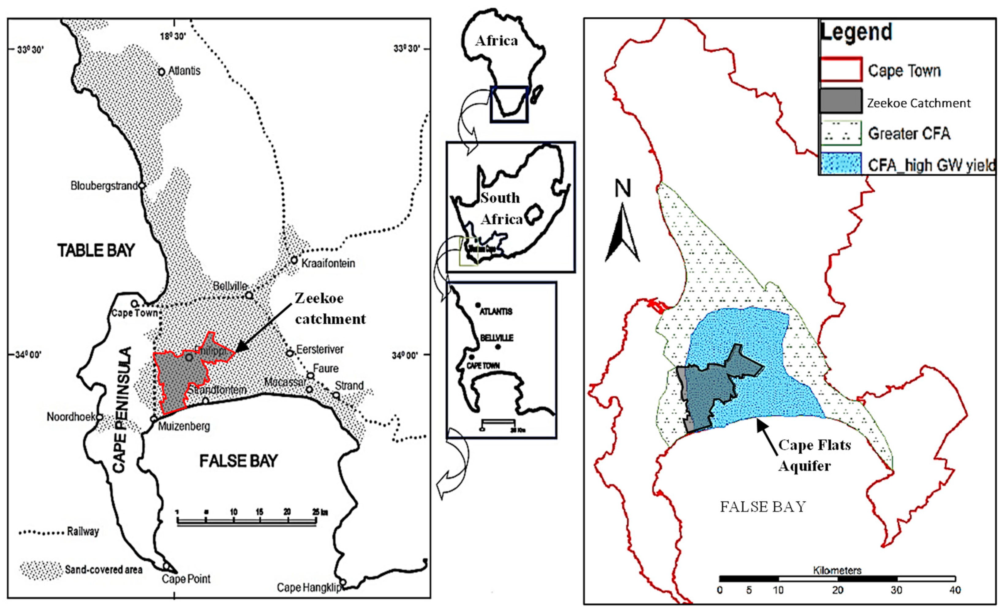
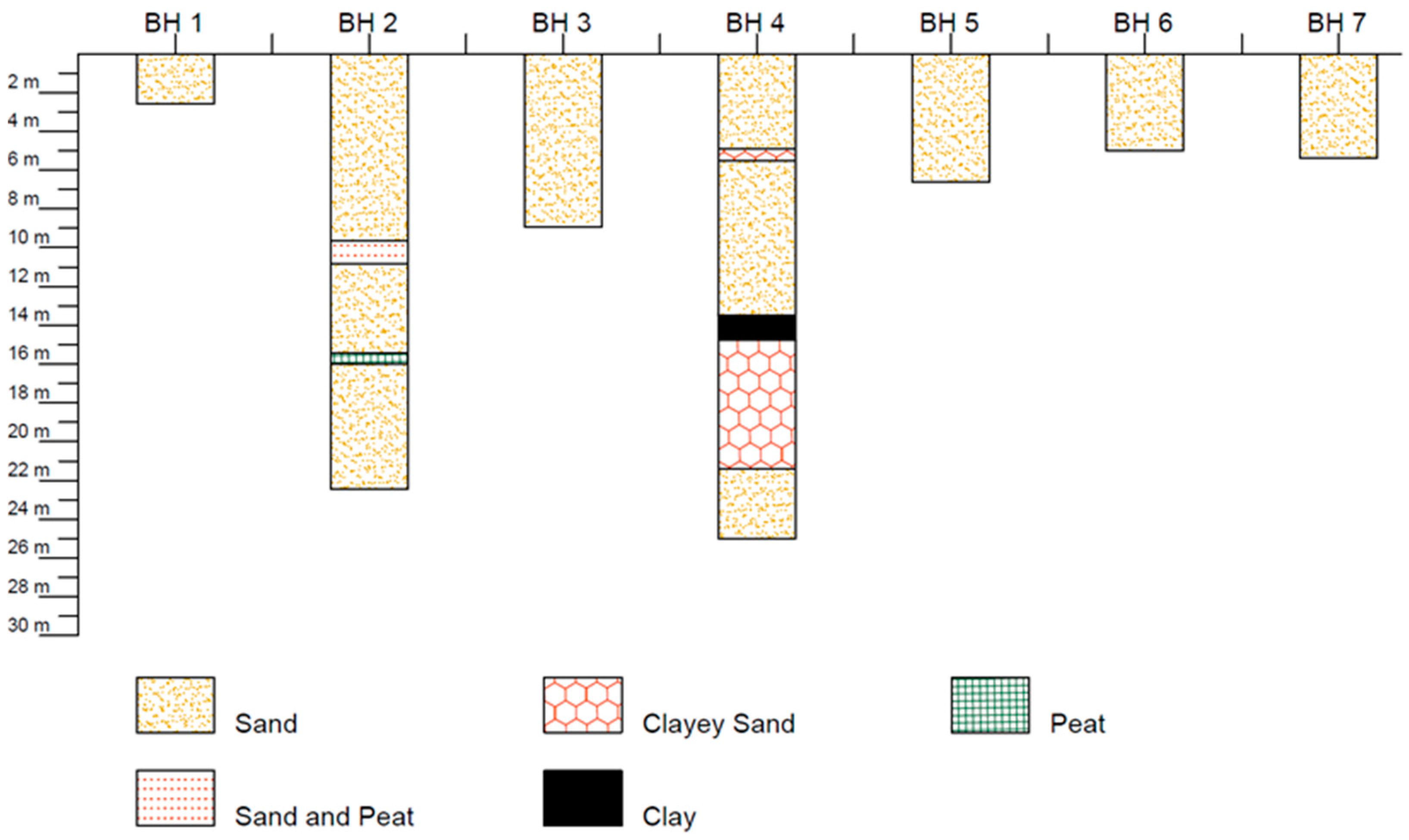
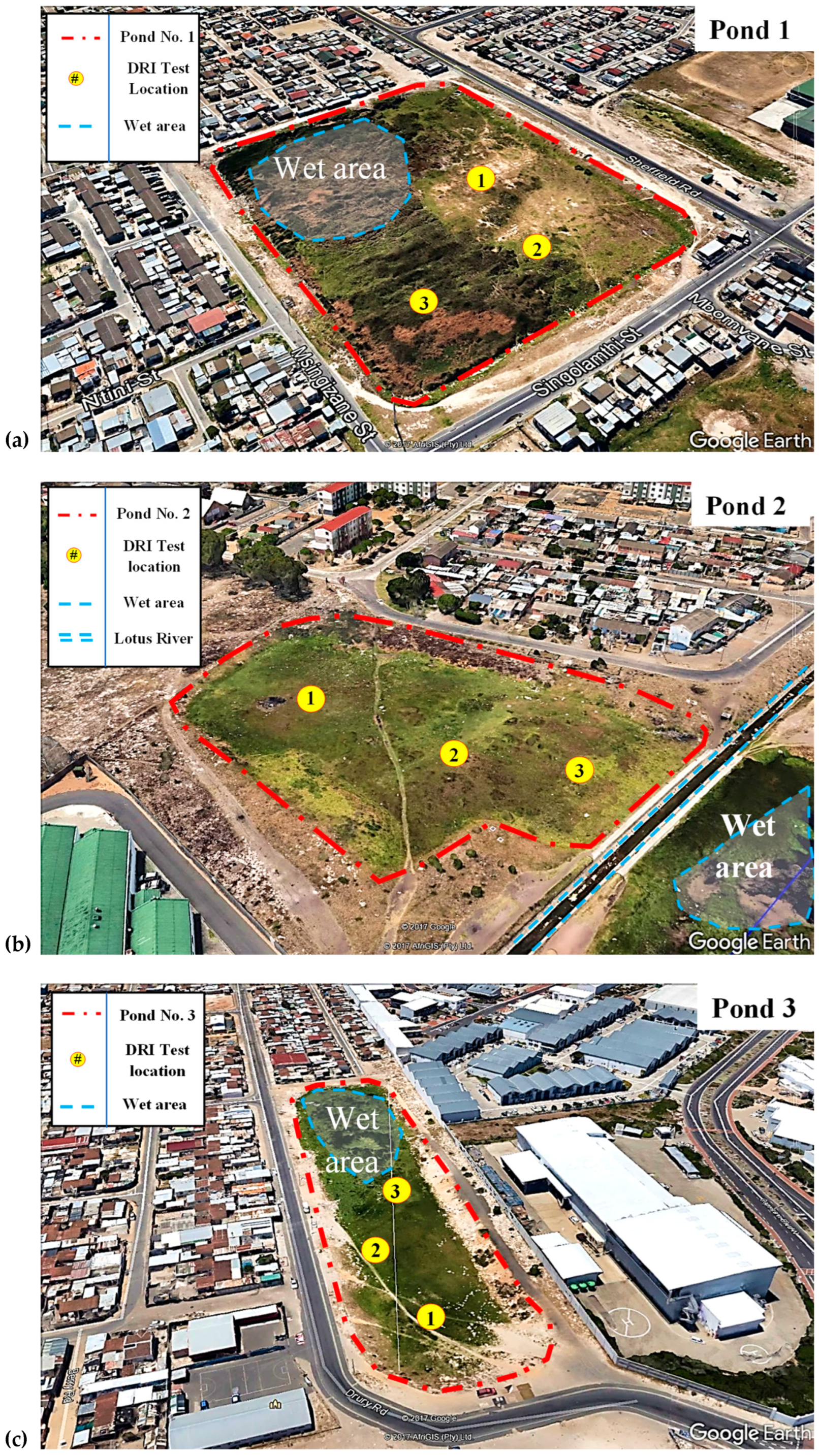
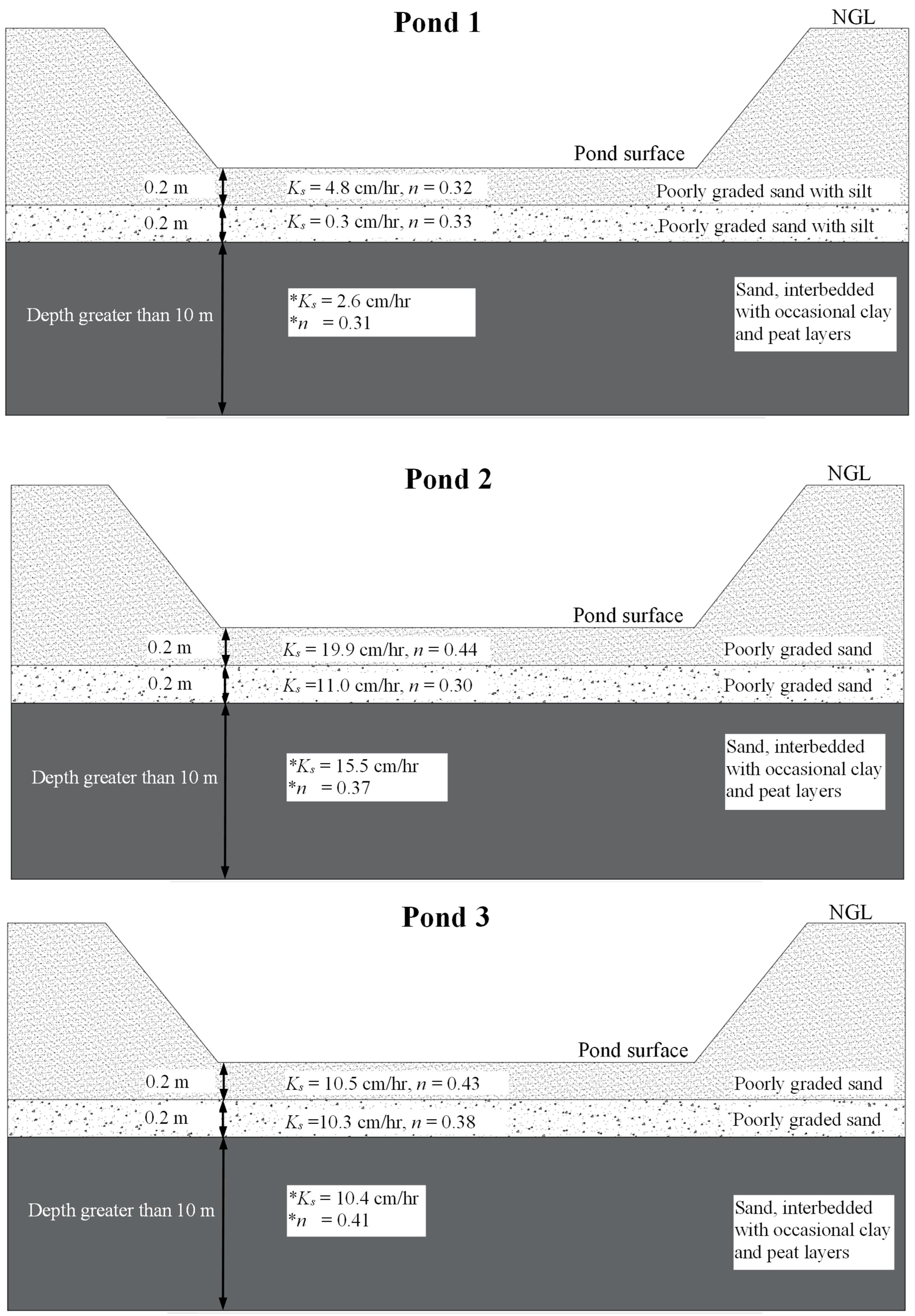
2.1. Study Area
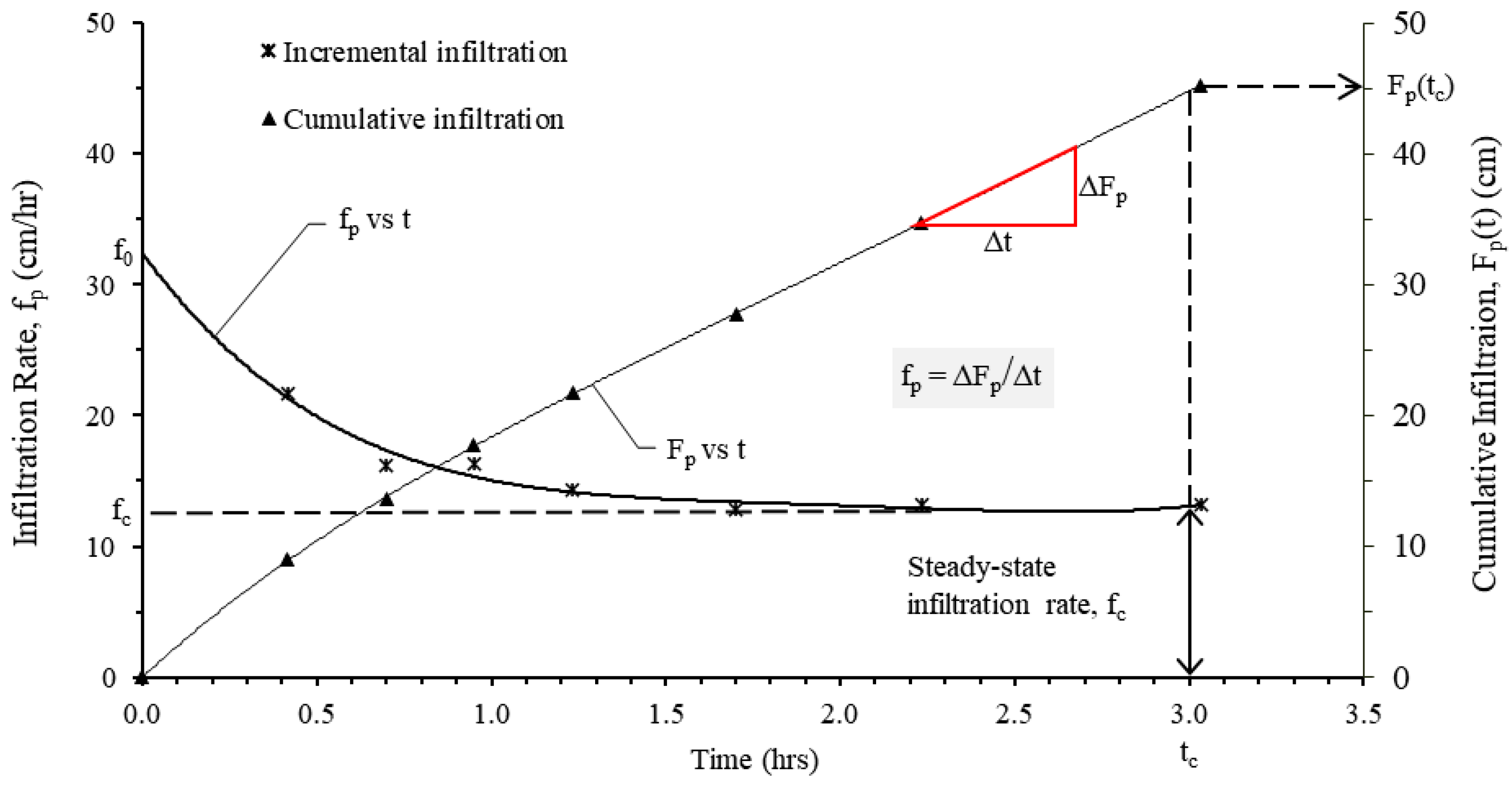
2.2. Field Tests
2.3. Laboratory Tests
2.4. HYDRUS-2D Models
- Small-scale models to replicate field infiltration tests;
- Large-scale models to estimate vertical water movement through the unsaturated zone to the water table, located approximately 5.5 m below the pond surfaces.
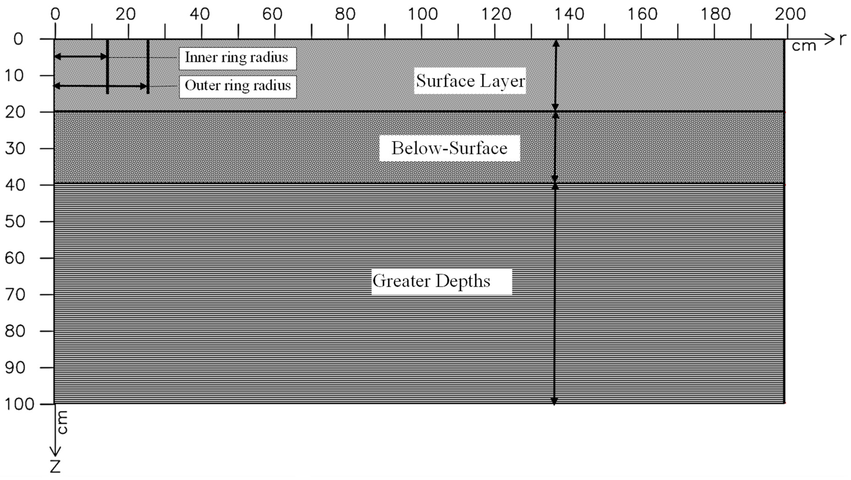
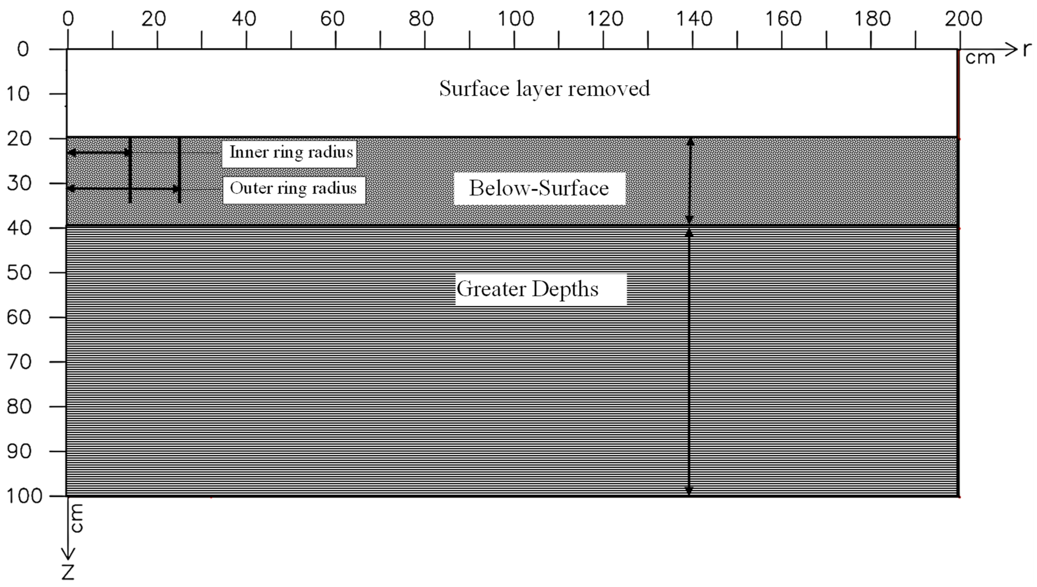
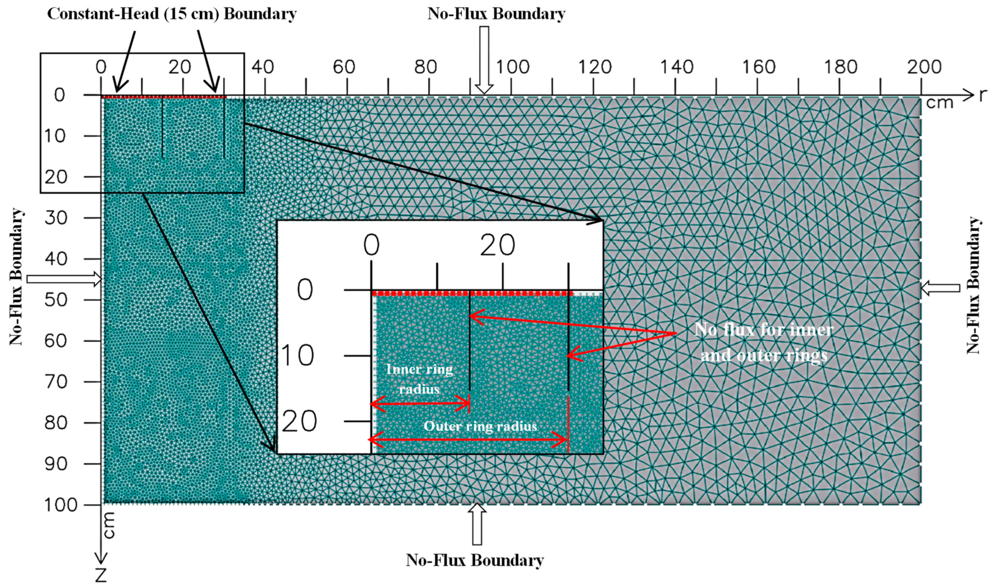
2.4.1. Simulation of Double-Ring Infiltrometer (DRI) Field Tests
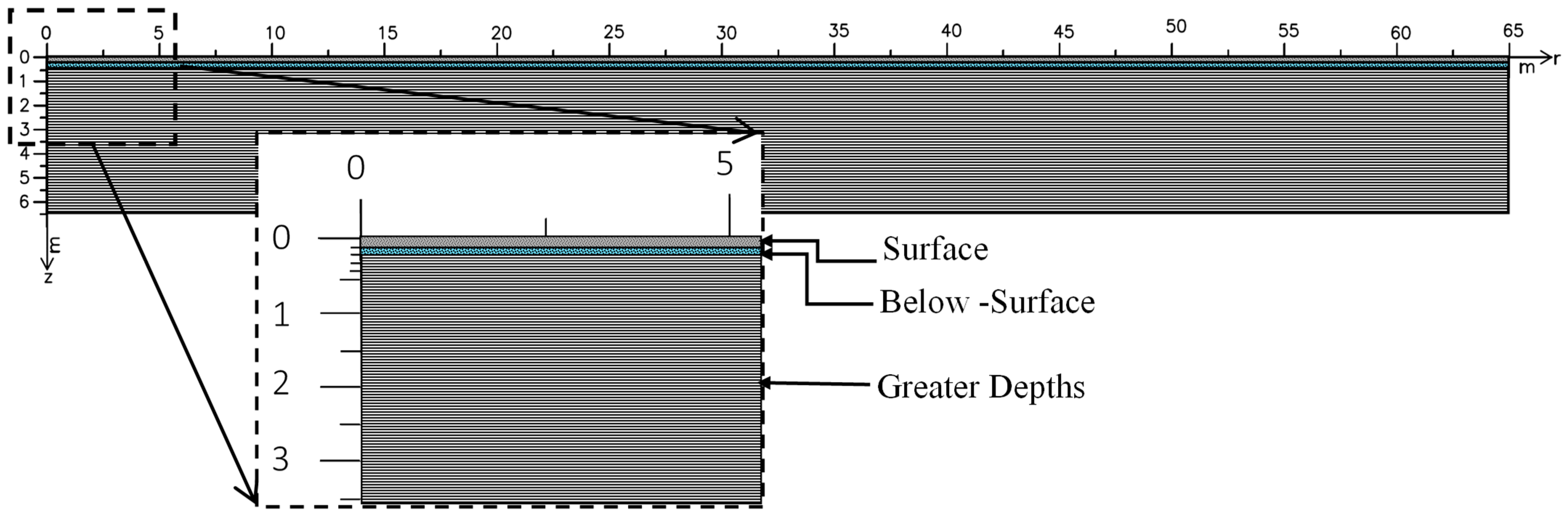
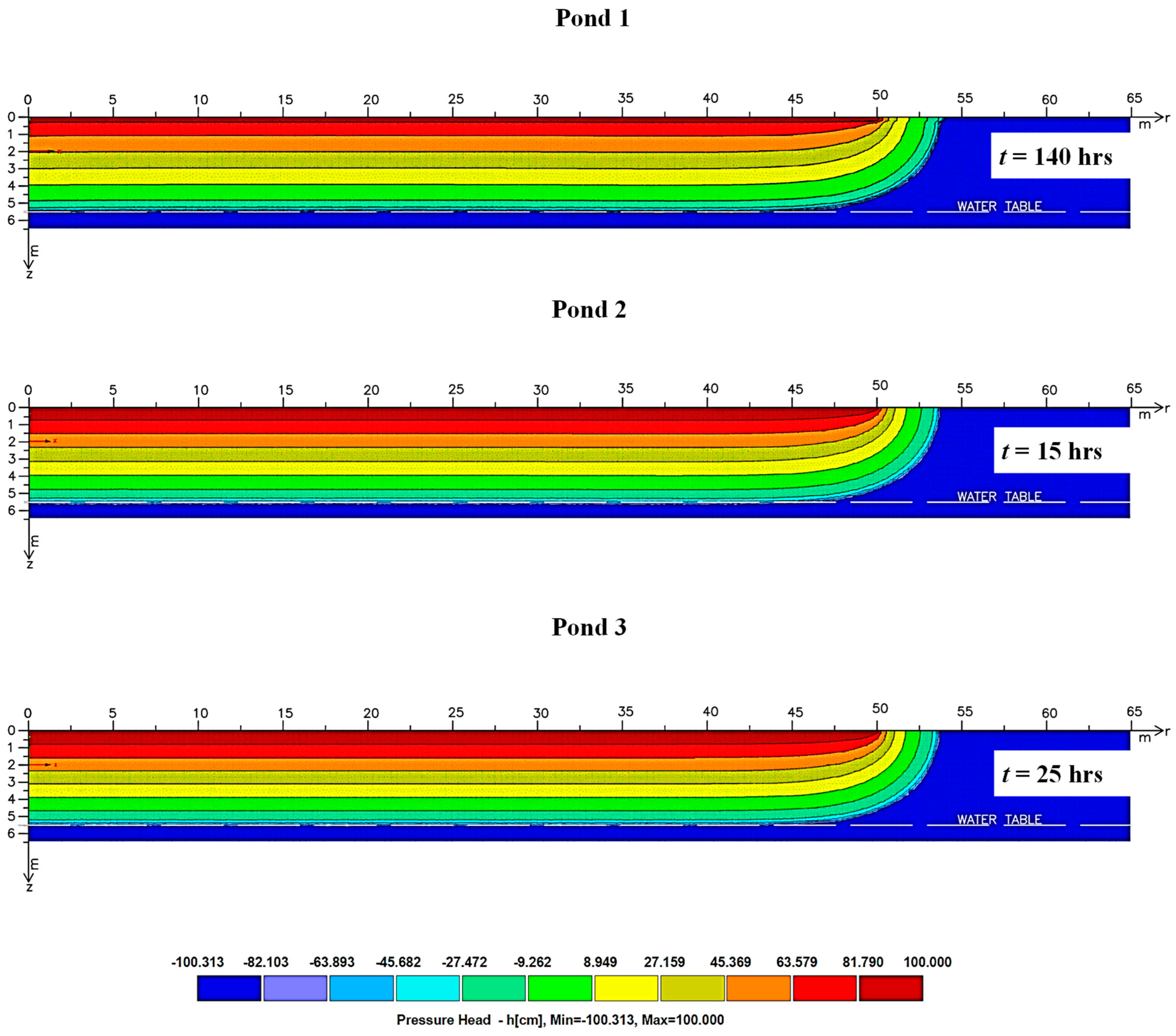
2.4.2. Simulation of Water Movement to the Water Table
3. Results
3.1. Field Results
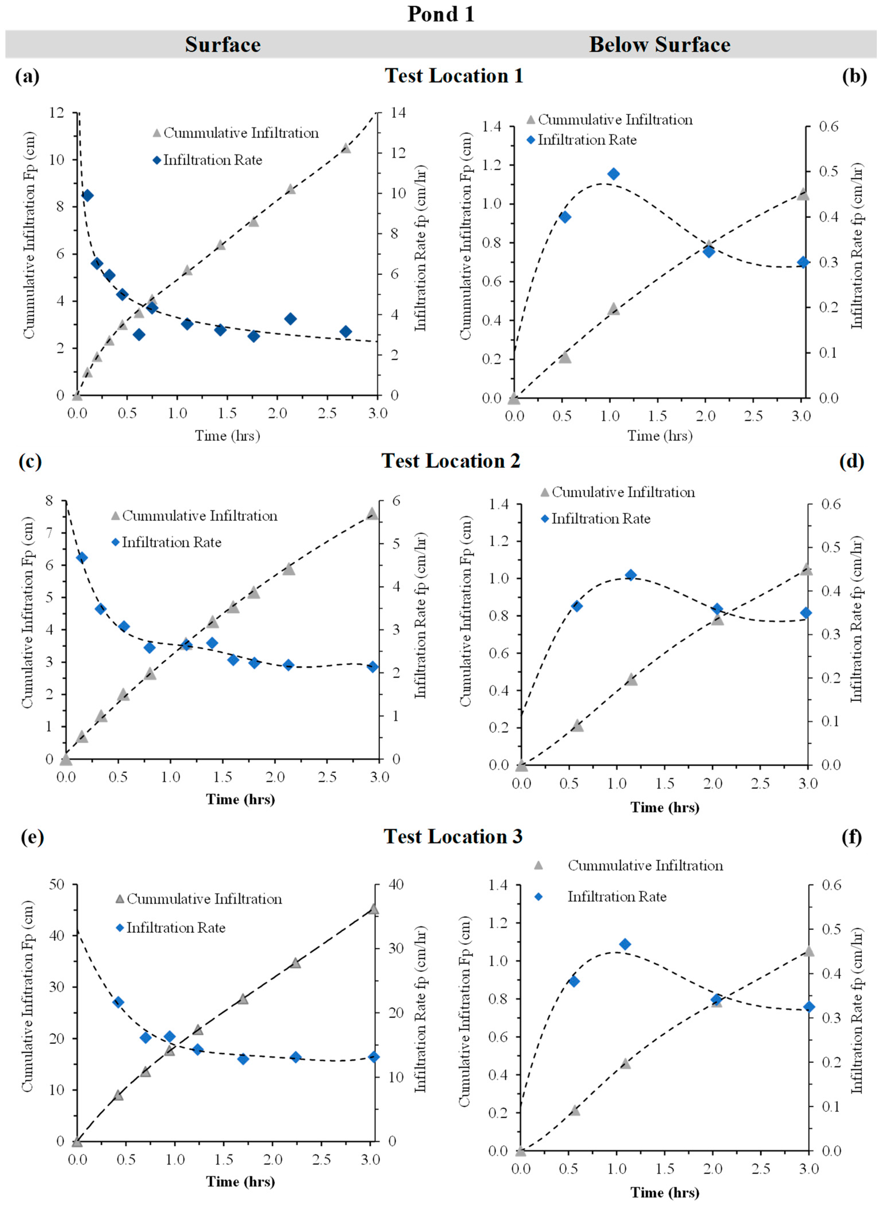
3.1.1. Infiltration Dynamics in Pond 1
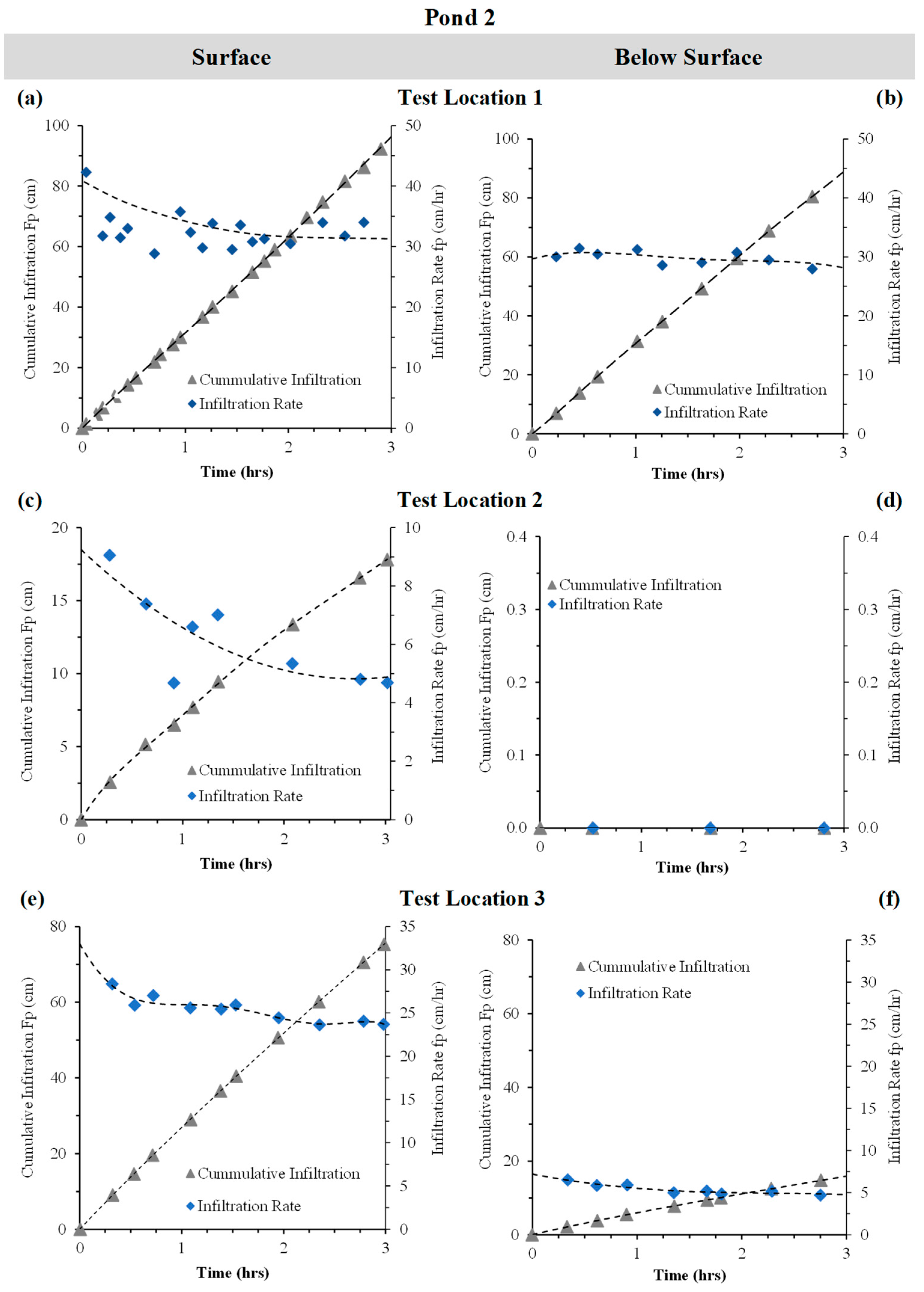
3.1.2. Infiltration Dynamics in Pond 2
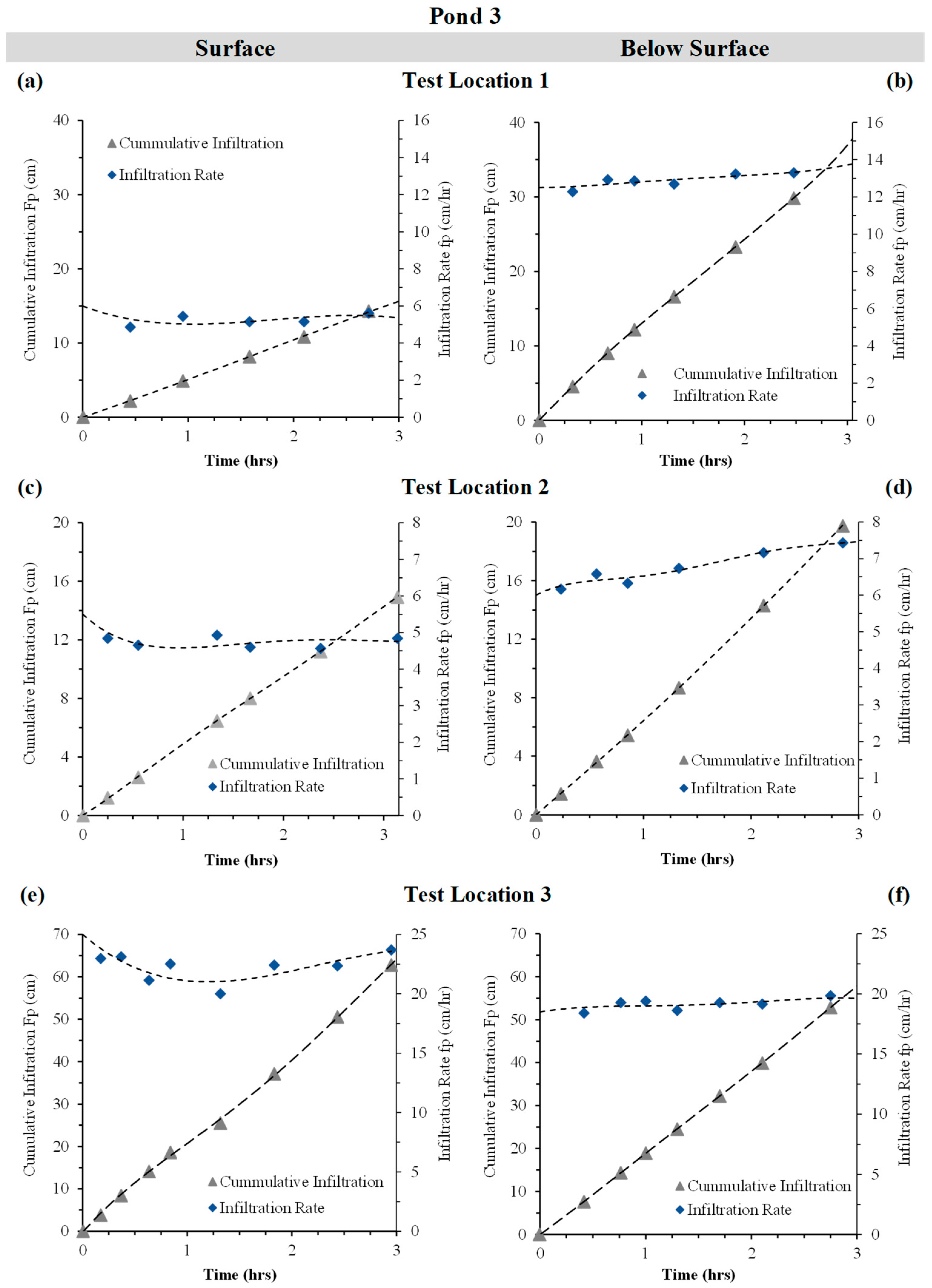
3.1.3. Infiltration Dynamics in Pond 3
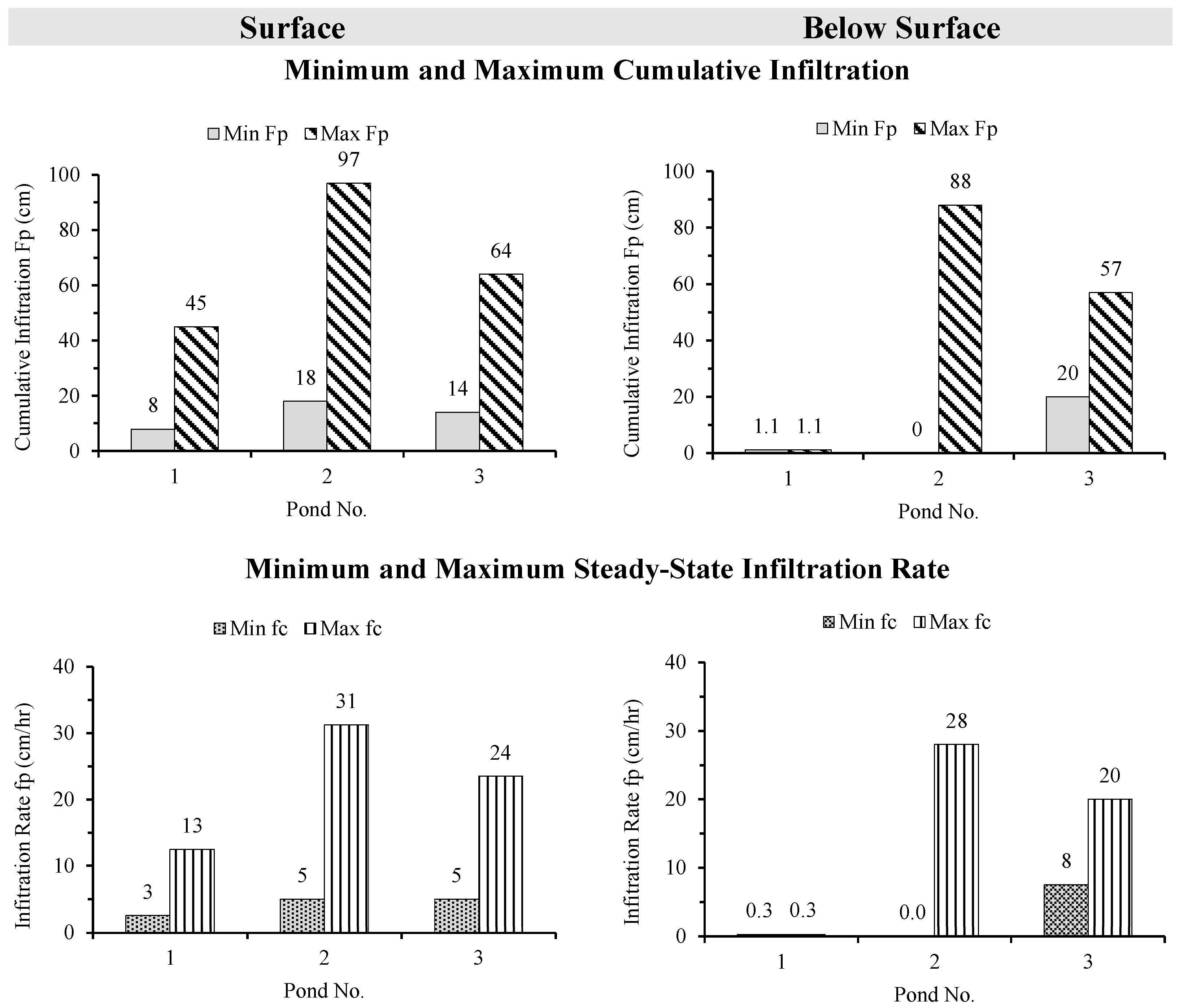
3.1.4. Comparison of Infiltration Ranges Across Ponds
3.1.5. Horton’s Decay Coefficient and Steady-State Infiltration Rate
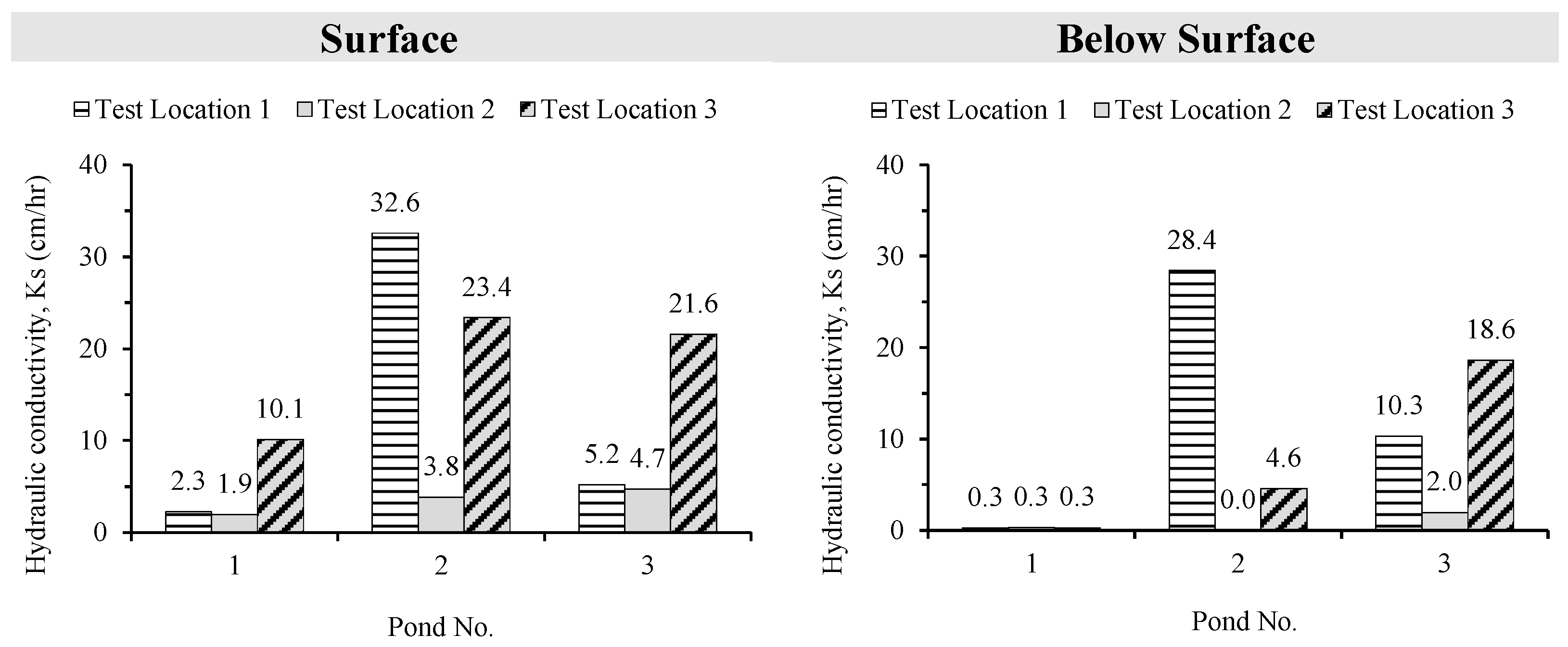
3.1.6. Hydraulic Conductivity Derived from Green–Ampt Parameters
3.2. Laboratory Results
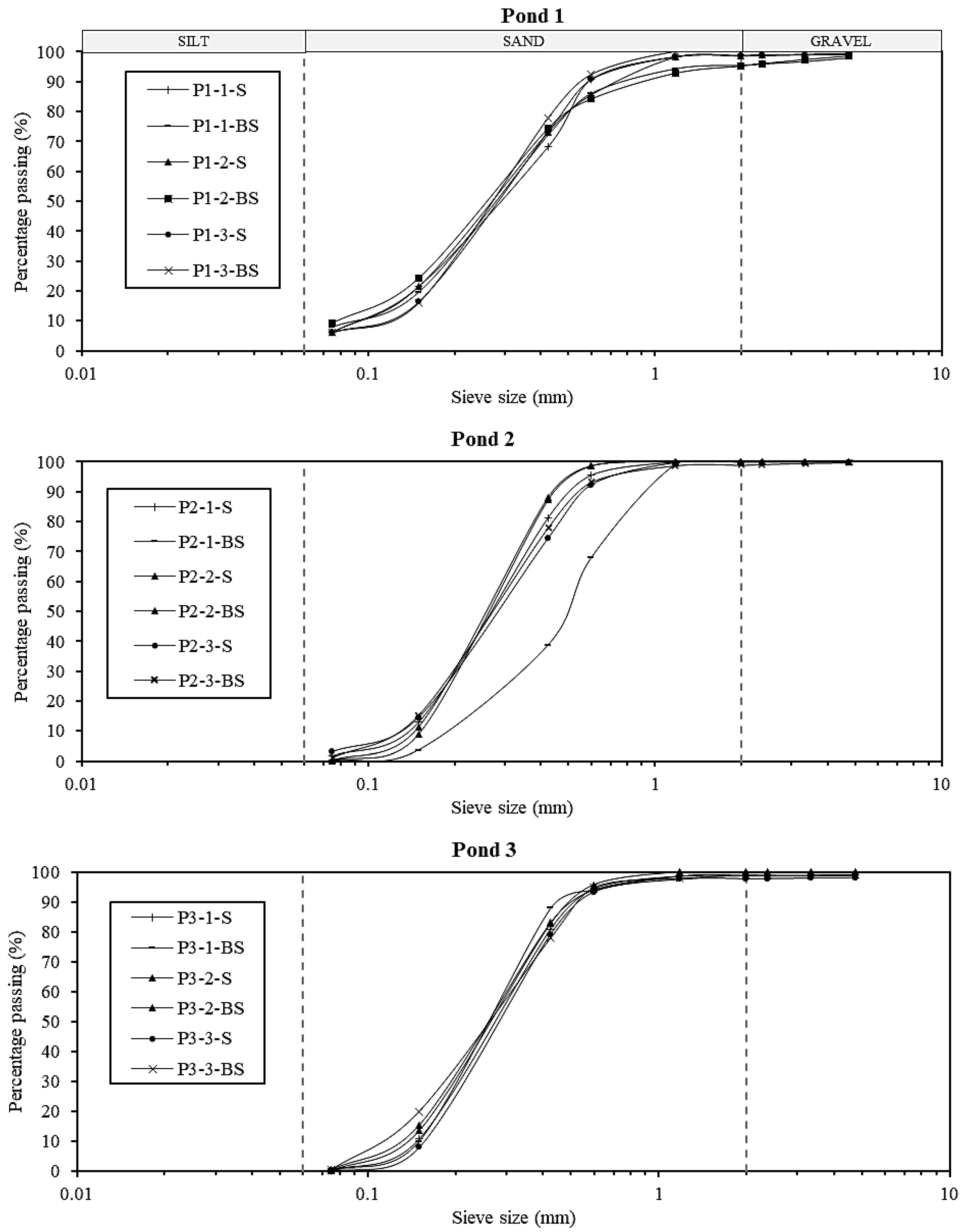
3.2.1. Particle Size Distribution
3.2.2. Flow Rates from Constant-Head Permeameter Tests
3.2.3. Hydraulic Conductivity from Laboratory Constant-Head Permeameter Test
3.3. Comparison Between Field and Laboratory Results
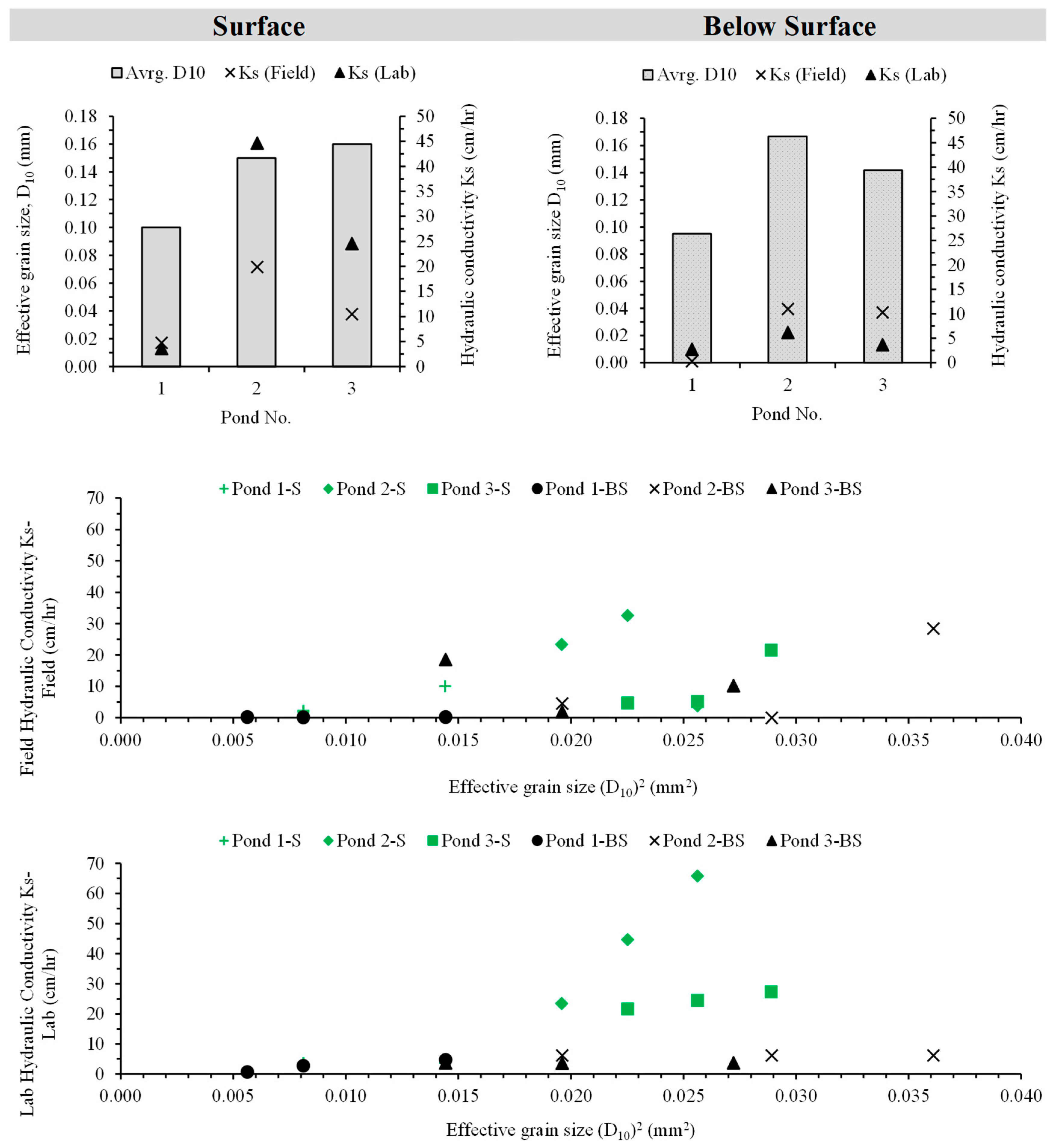
3.3.1. Hydraulic Conductivity Variation with Soil Effective Grain Size
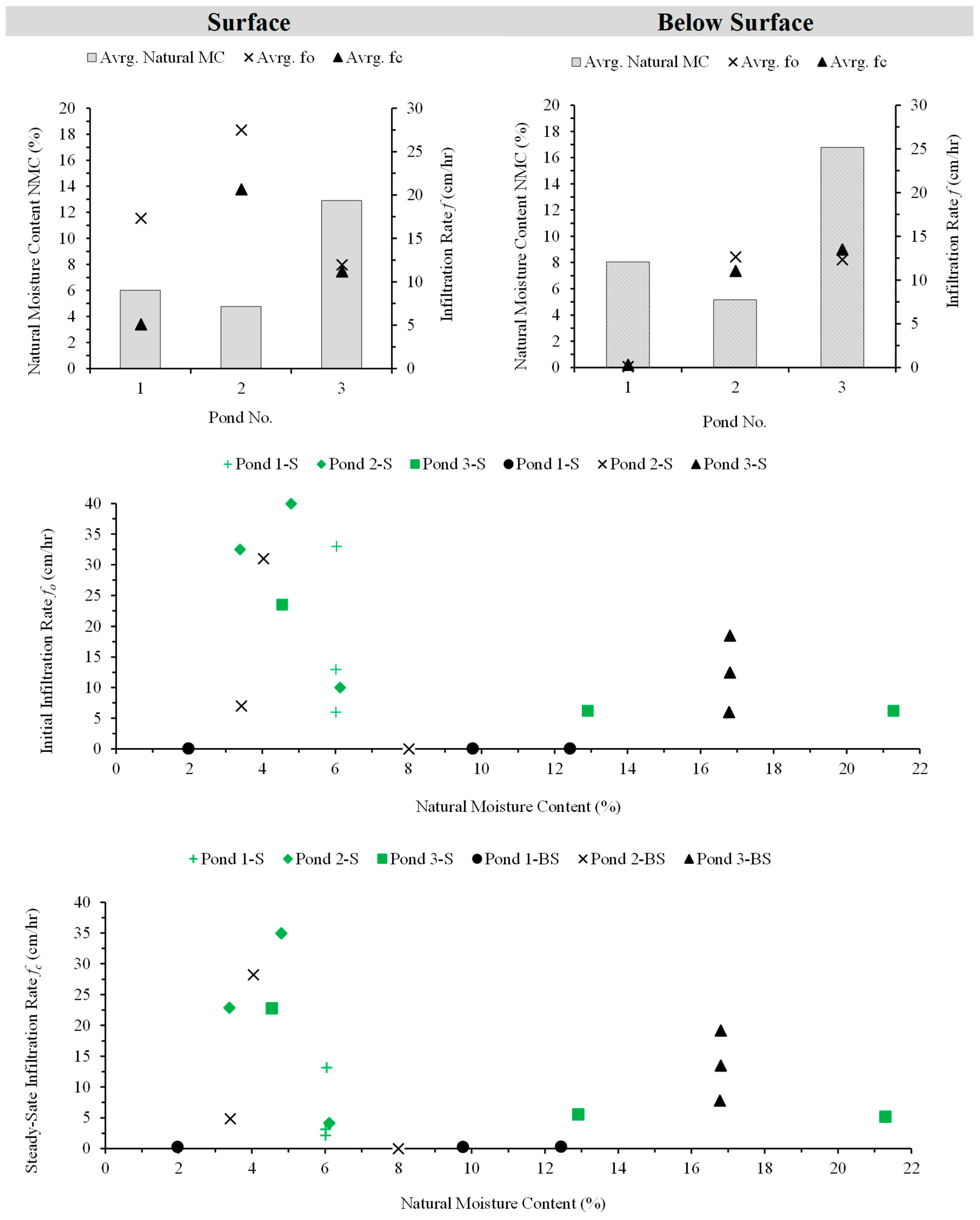
3.3.2. Influence of Moisture Content on Infiltration Rates
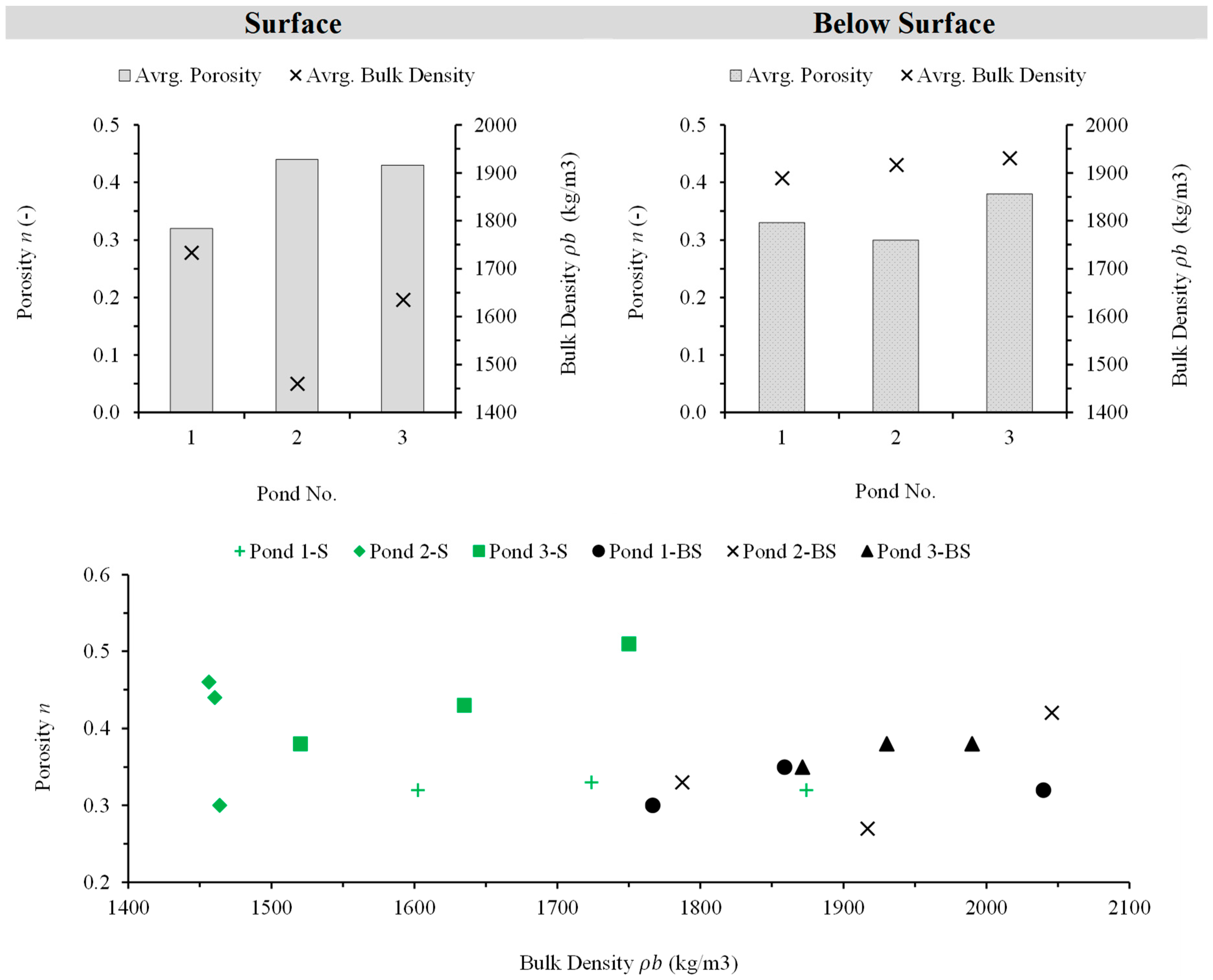
3.3.3. Relationship Between Porosity and Bulk Density
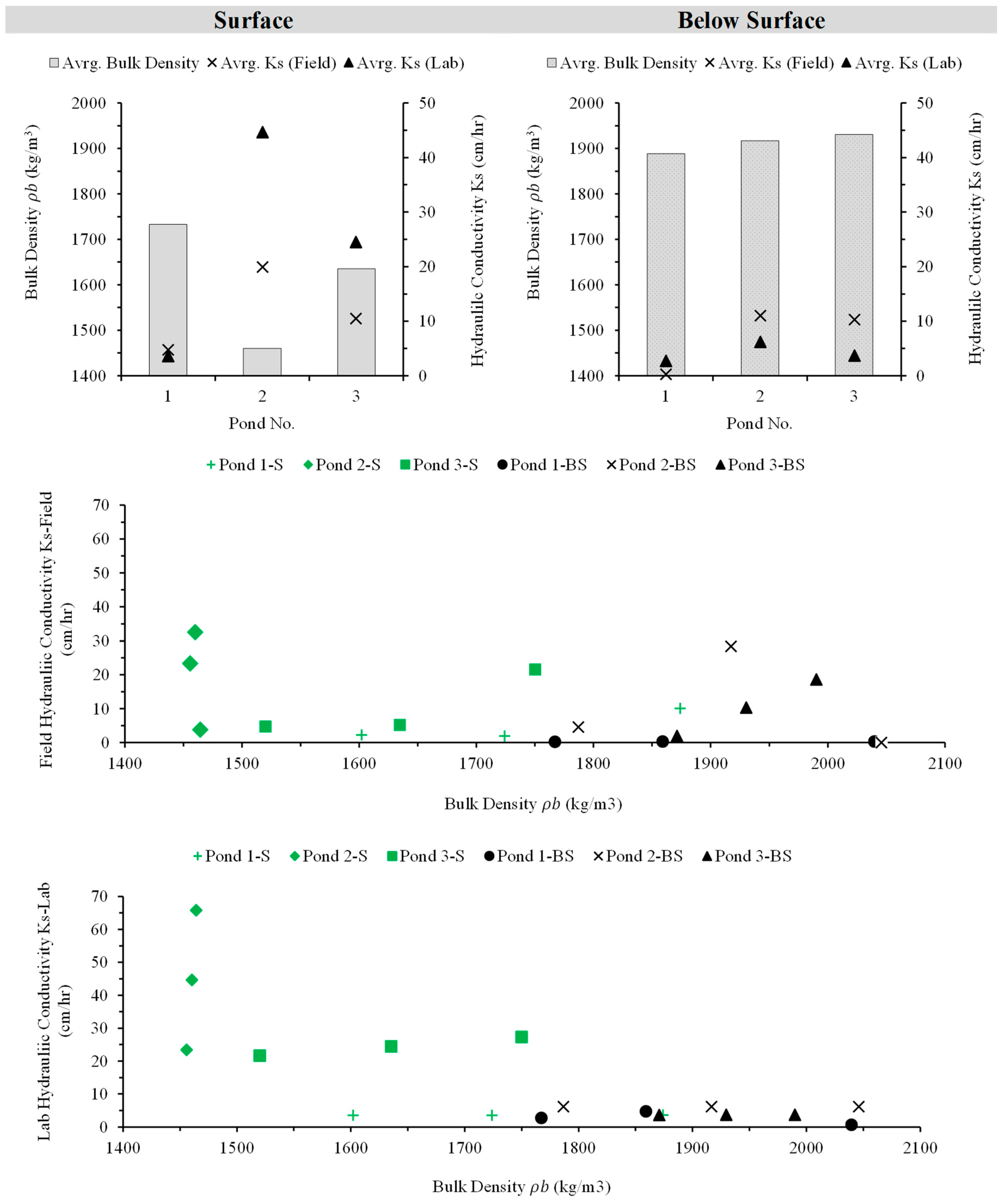
3.3.4. Hydraulic Conductivity Variation with Bulk Density
3.4. Summary of Experimental Results
3.5. HYDRUS-2D Simulation Results
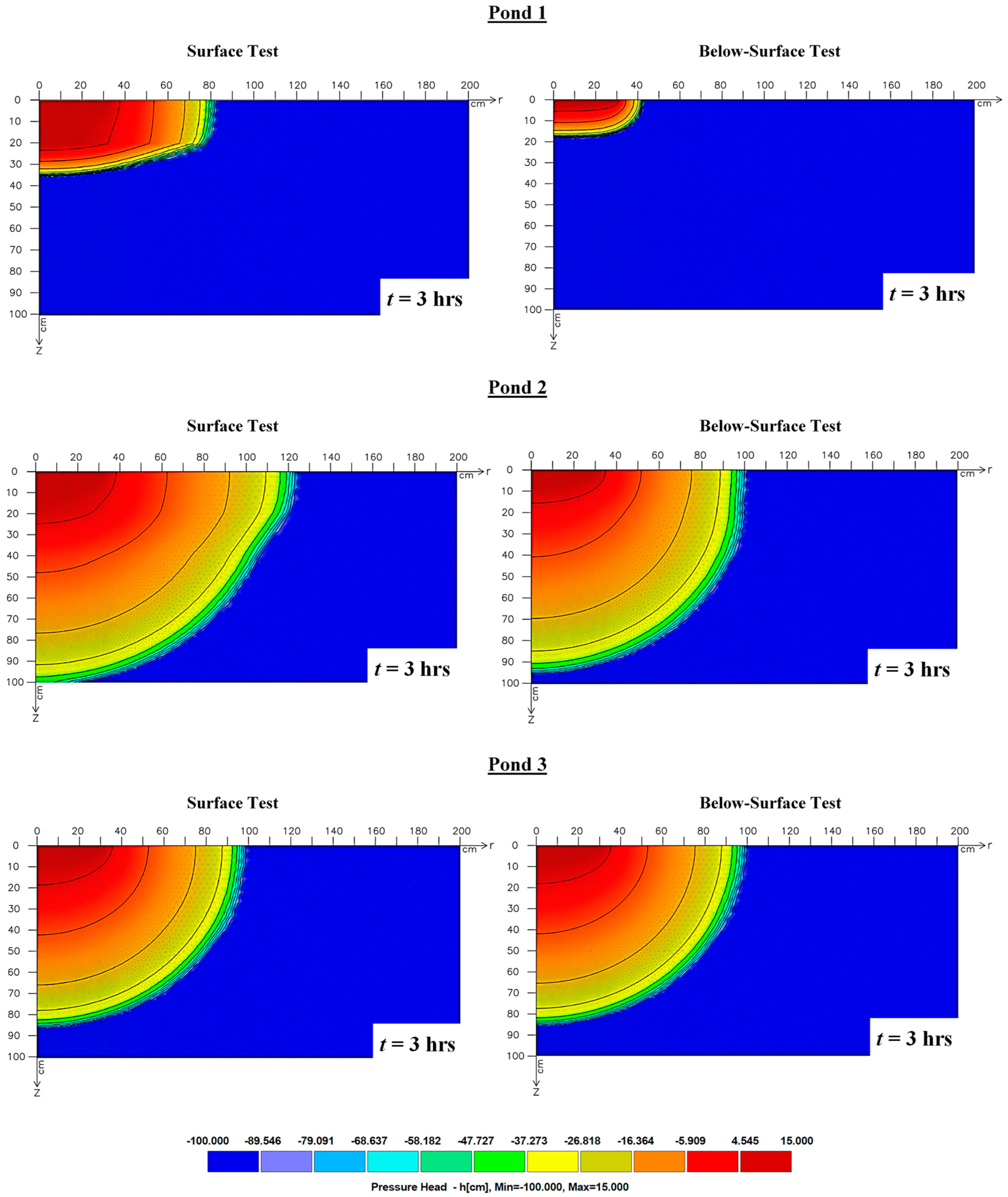
3.5.1. Simulation Results of Double-Ring Infiltrometer
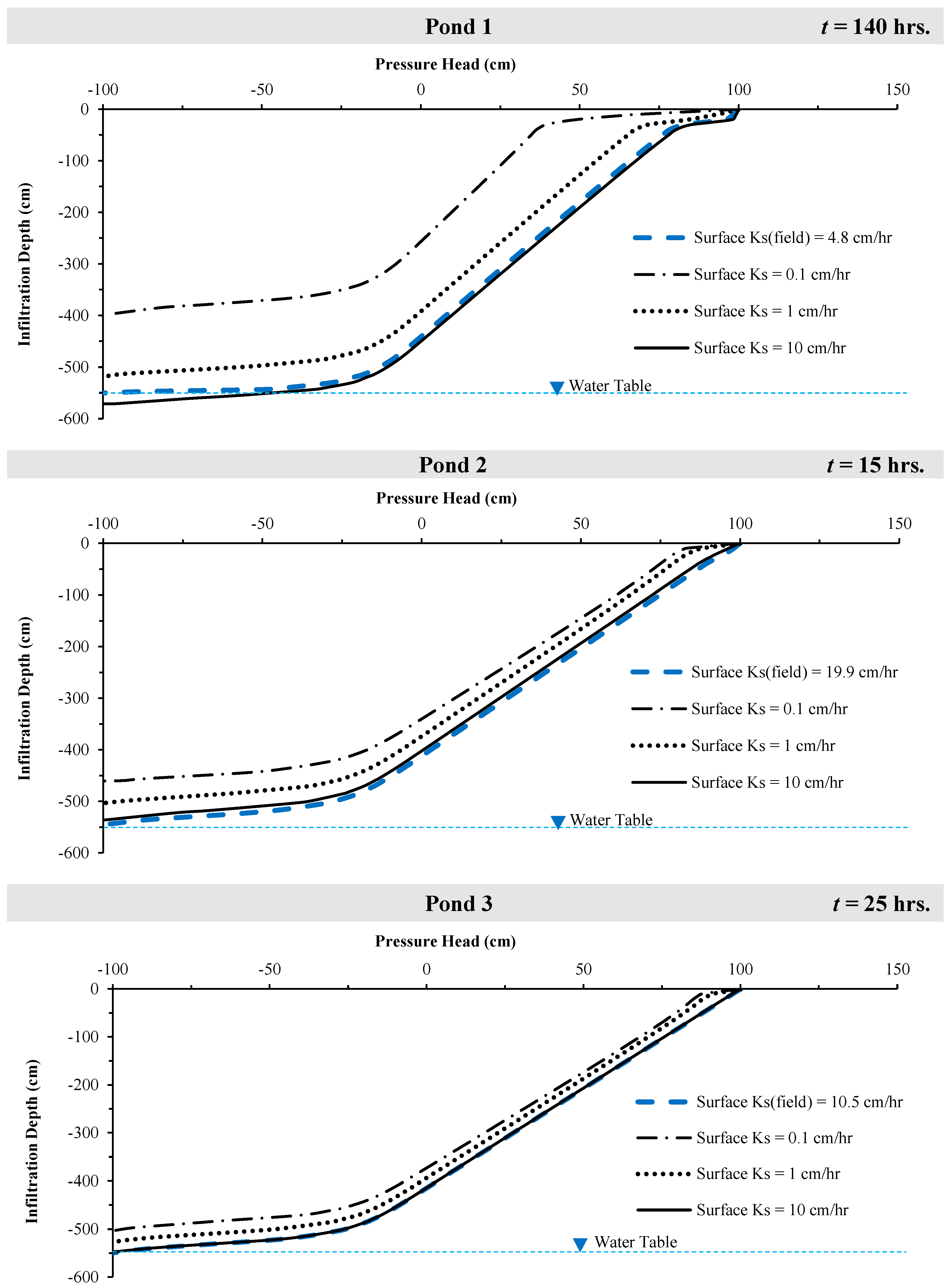
3.5.2. Simulation Results of Water Movement to the Water Table
3.6. Variation in Hydraulic Conductivity and Infiltration Rates
3.6.1. Discrepancies Between Field and Lab Hydraulic Conductivity Measurements
3.6.2. Comparison of Field-Measured and Simulated Infiltration Rates
4. Discussion
5. Conclusions
Author Contributions
Funding
Data Availability Statement
Acknowledgments
Conflicts of Interest
References
- Pitman, W.V. Overview of water resource assessment in South Africa: Current state and future challenges. Water SA 2011, 37, 659–664. [Google Scholar] [CrossRef]
- Mudefi, E. Perspectives on 2018 ‘water crisis management’ in Cape Town, South Africa: A systematic review. Int. J. Water 2023, 19, 248–274. [Google Scholar] [CrossRef]
- Warner, J.F.; Meissner, R. Cape Town’s “Day Zero” water crisis: A manufactured media event? Int. J. Disaster Risk Reduct. 2021, 64, 102481. [Google Scholar] [CrossRef]
- City of Cape Town. Water Outlook 2018 Report; Department of Water and Sanitation, City of Cape Town: Cape Town, South Africa, 2018. Available online: https://resource.capetown.gov.za/documentcentre/Documents/City%20research%20reports%20and%20review/Water%20Outlook%202018_Rev%2030_31%20December%202018.pdf (accessed on 15 January 2025).
- Stefan, C.; Ansems, N. Web-based global inventory of managed aquifer recharge applications. Sustain. Water Resour. Manag. 2018, 4, 153–162. [Google Scholar] [CrossRef]
- Dillon, P.; Toze, S.; Page, D.; Vanderzalm, J.; Bekele, E.; Sidhu, J.; Rinck-Pfeiffer, S. Managed aquifer recharge: Rediscovering nature as a leading edge technology. Water Sci. Technol. 2010, 62, 2338–2345. [Google Scholar] [CrossRef]
- Dillon, P.; Pavelic, P.; Page, D.; Beringen, H.; Ward, J. Managed Aquifer Recharge: An Introduction; Waterlines Report Series No. 13; National Water Commission: Canberra, Australia, 2009; pp. 1–76. Available online: https://recharge.iah.org/files/2016/11/MAR_Intro-Waterlines-2009.pdf (accessed on 10 March 2025).
- Page, D.; Vanderzalm, J.; Barry, K.; Levett, K.; Kremer, S.; Ayuso-Gabella, N.; Dillon, P.; Toze, S.; Sidhu, J.; Shackleton, M. Operational Residual Risk Assessment for the Salisbury Stormwater ASTR Project. In Water for a Healthy Country National Research Flagship Report; CSIRO: Perth, WA, Australia, 2009. [Google Scholar]
- Murray, R.; Tredoux, G.; Ravenscroft, P.; Botha, F. Artificial Recharge Strategy—Version 1.3. In Strategy Development: A National Approach to Implement Artificial Recharge as Part of Water Resource Planning; Department of Water Affairs and Forestry: Pretoria, South Africa, 2007. Available online: https://www.dws.gov.za/Documents/Other/Water%20Resources/ARStrategyforSAJun07SecA.pdf (accessed on 20 March 2025).
- Tredoux, G.; Van der Merwe, B.; Peters, I. Artificial recharge of the Windhoek aquifer, Namibia: Water quality considerations. Bol. Geol. Min. 2009, 120, 269–278. Available online: https://web.igme.es/Boletin/2009/120_2_2009/269-278.pdf (accessed on 5 March 2025).
- Wright, W.; Conrad, J. The Cape Flats Aquifer: Current Status; CSIR Report No. 11/95; CSIR: Stellenbosch, South Africa, 1995. Available online: https://www.dws.gov.za/ghreport/reports/2.2%28291%29.pdf (accessed on 10 January 2025).
- Okedi, J. The Prospects for Stormwater Harvesting in Cape Town, South Africa Using the Zeekoe Catchment as a Case Study. Ph.D. Thesis, University of Cape Town, Cape Town, South Africa, 2019. Available online: https://open.uct.ac.za/handle/11427/30453 (accessed on 30 June 2020).
- Tanyanyiwa, C.T.; Armitage, N.P.; Okedi, J. The hydrological impacts of retrofitted detention ponds for urban managed aquifer recharge in the Cape Flats, South Africa. Water 2025, 17, 145. [Google Scholar] [CrossRef]
- Tredoux, G.; Ross, W.; Gerber, A. The potential of the Cape Flats aquifer for the storage and abstraction of reclaimed effluent (South Africa). In Proceedings of the International Symposium on Artificial Groundwater Recharge, Dortmund, Germany, 14–18 May 1979; Volume 131, pp. 23–43. [Google Scholar]
- Vandoolaeghe, M.A.C. The Cape Flats Groundwater Development Pilot Abstraction Scheme; Technical Report Gh3655; Directorate Geohydrology: Cape Town, South Africa, 1989. Available online: https://www.dws.gov.za/ghreport/reports/GH3655.pdf (accessed on 15 March 2025).
- Mauck, B.; Winter, K. Assessing the potential for managed aquifer recharge (MAR) of the Cape Flats Aquifer. Water SA 2021, 47, 505–514. [Google Scholar] [CrossRef]
- Parsons, R. Groundwater Information Sheet: Cape Flats Aquifer; WRC Report No. TT 357/08; Water Research Commission: Pretoria, South Africa, 2008. [Google Scholar]
- Nel, M. Groundwater: The Myths, the Truths and the Basics; WRC Report No. SP 108/17; Water Research Commission: Gezina, South Africa, 2017; Available online: https://www.wrc.org.za/wp-content/uploads/mdocs/Groundwater%20book_web.pdf (accessed on 2 March 2025)ISBN 978-1-4312-0917-0.
- Tredoux, G.; Cain, J. The Atlantis Water Resource Management Scheme: 30 Years of Artificial Groundwater Recharge; Report No. PRSA 000/00/11609/10—Activity 17; Department of Water Affairs: Pretoria, South Africa, 2010.
- Bugan, R.D.H.; Jovanovic, N.; Israel, S.; Tredoux, G.; Genthe, B.; Steyn, M.; Allpass, D.; Bishop, R.; Marinus, V. Four decades of water recycling in Atlantis (Western Cape, South Africa): Past, present, and future. Water SA 2016, 42, 577–594. [Google Scholar] [CrossRef]
- Wright, A.; du Toit, I.D. Artificial recharge of urban wastewater: The key component in the development of an industrial town on the arid west coast of South Africa. Hydrogeol. J. 1996, 4, 118–129. [Google Scholar] [CrossRef]
- Tredoux, G.; Cavé, L.C.; Bishop, R. Long-term stormwater and wastewater infiltration into a sandy aquifer, South Africa. In Management of Aquifer Recharge for Sustainability, Proceedings of the 4th International Symposium on Artificial Recharge of Groundwater (ISAR-4), Adelaide, SA, Australia, 22–26 September 2002; Dillon, P.J., Ed.; CRC Press: Boca Raton, FL, USA, 2020. [Google Scholar]
- ASTM D3385-09; Standard Test Method for Infiltration Rate of Soils in the Field Using Double-Ring Infiltrometer. ASTM International: West Conshohocken, PA, USA, 2009. [CrossRef]
- Gregory, J.H. Stormwater Infiltration at the Scale of an Individual Residential Lot in North Central Florida. Master’s Thesis, University of Florida, Gainesville, FL, USA, 2004. Available online: https://buildgreen.ifas.ufl.edu/attachment/Stormwater_Infiltration_JustinGregory.pdf (accessed on 5 March 2025).
- Teague, N.F. Near Surface Infiltration Measurements and the Implications for Artificial Recharge. Master’s Thesis, San Diego State University, San Diego, CA, USA, 2010. Available online: https://www.researchgate.net/publication/274638738 (accessed on 2 March 2025).
- Dunkerley, D. Infiltration rates and soil moisture in a groved mulga community near Alice Springs, arid central Australia: Evidence for complex internal rainwater redistribution in a runoff–runon landscape. J. Arid Environ. 2002, 51, 199–219. [Google Scholar] [CrossRef]
- Kumar, P.A.; Vardhan, P.V.M.; Karishma, S.N. Study of soil infiltration rates on different soil conditions at selected sites. Int. J. Latest Trends Eng. Technol. 2017, 10, 223–227. [Google Scholar] [CrossRef]
- Boeno, D.; Gubiani, P.I.; Van Lier, Q.J.; Mulazzani, R.P. Estimating lateral flow in double ring infiltrometer measurements. Rev. Bras. Cienc. Solo 2021, 45, e0210027. [Google Scholar] [CrossRef]
- Li, M.; Liu, T.; Duan, L.; Luo, Y.; Ma, L.; Zhang, J.; Zhou, Y.; Chen, Z. The scale effect of double-ring infiltration and soil infiltration zoning in a semi-arid steppe. Water 2019, 11, 1457. [Google Scholar] [CrossRef]
- Van Vuuren, J.H.; Dippenaar, M.A.; Van Biljon, R.; Van Rooy, J.L. Seepage through permeable interlocking concrete pavements and their subgrades using a large infiltration table apparatus. Int. J. Pavement Res. Technol. 2021, 14, 337–347. [Google Scholar] [CrossRef]
- Fourie, A.B.; Strayton, G. Evaluation of a new method for the measurement of permeability in the field. J. S. A. Inst. Civ. Eng. 1996, 38, 10–14. Available online: https://journals.co.za/doi/pdf/10.10520/AJA10212019_23823 (accessed on 15 March 2025).
- Fairbrother Drill Company Ltd. Collection of Geotechnical Investigation and Drilling Reports from Various Cape Town Sites; Unpublished Internal Documents (Hardcopy, Obtained During Site Visit in 2017); Fairbrother Drill Company Ltd.: Cape Town, South Africa, 2010. [Google Scholar]
- Conrad, J.E. Groundwater Specialist Study—Cape Town International Airport Runway Re-Alignment and Associated Infrastructure Project; GEOSS Report No. 2014/06-10; GEOSS: Stellenbosch, South Africa, 2014. [Google Scholar]
- GEOSS. Geohydrological Assessment of a Proposed Belhar Residential Development; GEOSS Report No. 2013/07-18; GEOSS—Geohydrological and Spatial Solutions International (Pty) Ltd.: Stellenbosch, South Africa, 2013. [Google Scholar]
- Radcliffe, D.E.; Šimůnek, J. Soil Physics with HYDRUS: Modelling and Applications; CRC Press: Boca Raton, FL, USA, 2010. [Google Scholar]
- Šimůnek, J.; van Genuchten, M.T.; Šejna, M. Development and applications of the HYDRUS and STANMOD software packages and related codes. Vadose Zone J. 2008, 7, 587–600. [Google Scholar] [CrossRef]
- Šimůnek, J.; Šejna, M.; van Genuchten, M.T. Modeling nonequilibrium flow and transport processes using HYDRUS. Vadose Zone J. 2008, 7, 782–797. [Google Scholar] [CrossRef]
- Mavundla, K.P. An Experimental Study on the Infiltration Potential of Stormwater Ponds in Zeekoe Catchment, Cape Town, South Africa. Master’s Thesis, University of Cape Town, Cape Town, South Africa, 2022. Available online: http://hdl.handle.net/11427/37078 (accessed on 10 January 2024).
- Department of Water Affairs and Forestry (DWAF). The Assessment of Water Availability in the Berg Catchment (WMA 19) by Means of Water Resource-Related Models: Groundwater Model Report Volume 5—Cape Flats Aquifer Model; Umvoto Africa (Pty) Ltd.: Cape Town, South Africa; Ninham Shand (Pty) Ltd.: Pretoria, South Africa, 2008. Available online: https://www.dws.gov.za/Documents/Other/WMA/19/Reports/Rep9-Vol5-GW%20Cape%20Flats%20Aquifer.pdf (accessed on 15 April 2021).
- Adelana, S.M.A.; Xu, Y.; Vrbka, P. A conceptual model for the development and management of the Cape Flats aquifer, South Africa. Water SA 2010, 36, 461–474. [Google Scholar] [CrossRef]
- Horton, R.E. The role of infiltration in the hydrologic cycle. Trans. Am. Geophys. Union 1933, 14, 446–460. [Google Scholar] [CrossRef]
- Green, W.H.; Ampt, G.A. Studies on soil physics: 1. The flow of air and water through soils. J. Agric. Sci. 1911, 4, 1–24. [Google Scholar] [CrossRef]
- Darcy, H. Les Fontaines Publiques de la Ville de Dijon; Dalmont: Paris, France, 1856; Available online: https://gallica.bnf.fr/ark:/12148/bpt6k624312 (accessed on 15 May 2021).
- Yu, C.; Zheng, C. HYDRUS: Software for Flow and Transport Modeling in Variably Saturated Media, Software Spotlight. Ground Water 2010, 48, 787–791. [Google Scholar] [CrossRef]
- Morianou, G.; Kourgialas, N.N.; Karatzas, G.P. A review of HYDRUS 2D/3D applications for simulations of water dynamics, root uptake and solute transport in tree crops under drip irrigation. Water 2023, 15, 741. [Google Scholar] [CrossRef]
- Fatehnia, M. Automated Method for Determining Infiltration Rate in Soils. Ph.D. Thesis, Florida State University, Tallahassee, FL, USA, 2015. [Google Scholar]
- ASTM D2487-17; Standard Practice for Classification of Soils for Engineering Purposes (Unified Soil Classification System). ASTM International: West Conshohocken, PA, USA, 2017. [CrossRef]
- Beyer, W. Zur Bestimmung der Wasserdurchlässigkeit von Kiesen und Sanden aus der Kornverteilungskurve. Wasserwirtsch. Wassertech. 1964, 14, 165–168. (In German) [Google Scholar]
- Subramanya, K. Engineering Hydrology, 3rd ed.; Tata McGraw-Hill Publishing Company Limited: New Delhi, India, 2008. [Google Scholar]
- Valentin, C.; Bresson, L.M. Morphology, genesis, and classification of surface crusts in loamy and sandy soils. Geoderma 1992, 55, 225–245. [Google Scholar] [CrossRef]
- Moriasi, D.N.; Arnold, J.G.; Van Liew, M.W.; Bingner, R.L.; Harmel, R.D.; Veith, T.L. Model evaluation guidelines for systematic quantification of accuracy in watershed simulations. Trans. ASABE 2007, 50, 885–900. [Google Scholar] [CrossRef]
- Weiss, P.T.; LeFevre, G.; Gulliver, J.S. Contamination of Soil and Groundwater Due to Stormwater Infiltration Practices: A Literature Review; Minnesota Pollution Control Agency: St. Paul, MN, USA, 2008; Available online: https://hdl.handle.net/11299/115341 (accessed on 28 July 2023).


| Pond No. | Pond Type | Surface Area (m2) | Latitude | Longitude |
|---|---|---|---|---|
| 1 | Detention | 32,000.0 | −34.009 | 18.581 |
| 2 | Retention | 10,000.0 | −34.025 | 18.519 |
| 3 | Detention | 9000.0 | −34.087 | 18.484 |
| Description | Parameter | Unit | Magnitude |
|---|---|---|---|
| Time Discretisation | Initial | hour | 0 |
| Final | hour | 3 | |
| Initial time step | hour | 0.0024 | |
| Minimum time step | hour | 0.00024 | |
| Maximum time step | hour | 120 | |
| Number of print time | hour | 10 | |
| Iteration | Maximum number of iterations | - | 10 |
| Water content tolerance | - | 0.001 | |
| Pressure head tolerance | cm | 1 | |
| Rectangular dimensions | Horizontal rectangular dimension | cm | 200 |
| Vertical rectangular dimension | cm | 100 | |
| FE mesh size | cm | 1–5 | |
| Boundary conditions | Top | - | Constant head and no-flux |
| Bottom | - | No flux | |
| Right side | - | No flux | |
| Left side | - | No flux |
| Description | Parameter | Unit | Magnitude |
|---|---|---|---|
| Time Discretisation | Initial | hour | 0 |
| Final | hour | 140 | |
| Initial time step | hour | 0.0024 | |
| Minimum time step | hour | 0.00024 | |
| Maximum time step | hour | 120 | |
| Number of print time | hour | 100 | |
| Iteration | Maximum number of iterations | - | 10 |
| Water content tolerance | - | 0.001 | |
| Pressure head tolerance | cm | 1 | |
| Rectangular dimensions | Horizontal rectangular dimension | cm | 6500 |
| Vertical rectangular dimension | cm | 650 | |
| FE mesh size | cm | 20 | |
| Boundary conditions | Top | - | Constant head |
| Bottom | - | Seepage face | |
| Right side | - | No flux | |
| Left side | - | No flux |
| Pond No. | C Constant | Ks,Beyer | Ks,field | Ks,lab |
|---|---|---|---|---|
| - | - | cm/h | cm/h | cm/h |
| Surface | ||||
| Pond 1 | 9.7 × 10⁻³ | 35.0 | 4.8 | 3.6 |
| Pond 2 | 1.1 × 10⁻² | 86.4 | 19.9 | 44.7 |
| Pond 3 | 1.1 × 10⁻² | 99.4 | 10.5 | 24.5 |
| Below Surface | ||||
| Pond 1 | 9.7 × 10⁻³ | 31.6 | 0.3 | 2.7 |
| Pond 2 | 1.0 × 10⁻² | 104.8 | 11.0 | 6.2 |
| Pond 3 | 1.1 × 10⁻² | 77.2 | 10.3 | 3.7 |
| Property | Notation | Units | Pond 1 | Pond 2 | Pond 3 | |||
|---|---|---|---|---|---|---|---|---|
| * Surface | ** Below Surface | * Surface | ** Below Surface | * Surface | ** Below Surface | |||
| Soil Texture | Fines | % | 6 | 8 | 2 | 1 | 1 | 1 |
| Sand | 92 | 89 | 98 | 99 | 98 | 98 | ||
| Gravel | 1 | 3 | 0 | 0 | 1 | 1 | ||
| Effective Grain Size | D10 | mm | 0.10 | 0.10 | 0.15 | 0.17 | 0.16 | 0.14 |
| D30 | 0.19 | 0.19 | 0.20 | 0.25 | 0.21 | 0.19 | ||
| D60 | 0.35 | 0.33 | 0.32 | 0.39 | 0.32 | 0.30 | ||
| Coefficients of Uniformity | Cu | - | 3.53 | 3.57 | 2.15 | 2.32 | 1.30 | 1.36 |
| Coefficients of Curvature | Cc | - | 1.01 | 1.14 | 0.85 | 0.98 | 0.85 | 0.86 |
| USCS Soil Group | - | - | SP-SM | SP-SM | SP | SP | SP | SP |
| Porosity | n | - | 0.32 | 0.33 | 0.44 | 0.30 | 0.43 | 0.38 |
| Void Ratio | e | % | 47 | 49 | 78 | 43 | 77 | 61 |
| Specific Gravity | GS | - | 2.61 | 2.60 | 2.49 | 2.60 | 2.56 | 2.58 |
| Bulk Density | ρb | kg/m3 | 1733 | 1889 | 1460 | 1917 | 1635 | 1930 |
| Natural Moisture Content | NMC | % | 6 | 8 | 5 | 5 | 13 | 17 |
| Lab Hydraulic Gradient | i | cm/cm | 9.7 | 9.7 | 9.8 | 9.6 | 9.7 | 9.7 |
| Lab Average Flow Rate | q | cm/h | 4 | 3 | 49.3 | 8.2 | 26.8 | 4 |
| Lab Hydraulic Conductivity | Ks,lab | cm/h | 3.6 | 2.8 | 44.7 | 6.2 | 24.5 | 3.7 |
| Field Hydraulic Conductivity | Ks,field | cm/h | 4.8 | 0.3 | 19.9 | 11 | 10.5 | 10.3 |
| Field Initial Infiltration Rate | fo | cm/h | 17.3 | 0.1 | 27.5 | 12.7 | 12 | 12.3 |
| Field Steady Infiltration Rate | fc | cm/h | 6.2 | 0.3 | 20.7 | 11 | 11.2 | 13.5 |
| Field Cum. Infiltration Rate | Fp | cm | 21.2 | 1.1 | 63.3 | 35.3 | 31.0 | 38.2 |
| Decay Coefficient | λ | - | 1.9 | 2.0 | 0.4 | 0.4 | 0.2 | 1.2 |
| Pond | Duration (Hours) | Surface Layer Ks (cm/h) | Wetting Front Depth (cm) | Infiltration Rate fp (cm/h) |
|---|---|---|---|---|
| Pond 1 | 140 | * 4.8 | 550 | 3.9 |
| 0.1 | 398 | 2.8 | ||
| 1.0 | 519 | 3.7 | ||
| 10.0 | 571 | 4.1 | ||
| Pond 2 | 15 | * 19.9 | 550 | 36.7 |
| 0.1 | 461 | 30.7 | ||
| 1.0 | 503 | 33.5 | ||
| 10.0 | 536 | 35.7 | ||
| Pond 3 | 25 | * 10.5 | 550 | 22.0 |
| 0.1 | 503 | 20.1 | ||
| 1.0 | 523 | 20.9 | ||
| 10.0 | 548 | 21.9 |
| (a) | ||||||||||||
| Field (Surface) | Field (Below Surface) | |||||||||||
| Pond No. | Test Loc. | Ks,field | Avg. Ks,field | Std. Dev. | CV | Pond No. | Test Loc. | Ks,field | Avg. Ks,field | Std. Dev. | CV | |
| - | - | cm/h | cm/h | - | % | - | - | cm/h | cm/h | - | % | |
| 1 | 1 | 2.3 | 4.8 | 4.6 | 97.0 | 1 | 1 | 0.3 | 0.3 | 0.0 | 0.0 | |
| 2 | 1.9 | 2 | 0.3 | |||||||||
| 3 | 10.1 | 3 | 0.3 | |||||||||
| 2 | 1 | 32.6 | 19.9 | 14.7 | 73.8 | 2 | 1 | 28.4 | 11.0 | 15.2 | 138.6 | |
| 2 | 3.8 | 2 | 0 | |||||||||
| 3 | 23.4 | 3 | 4.6 | |||||||||
| 3 | 1 | 5.2 | 10.5 | 9.6 | 91.6 | 3 | 1 | 10.3 | 10.3 | 8.3 | 80.6 | |
| 2 | 4.7 | 2 | 2 | |||||||||
| 3 | 21.6 | 3 | 18.6 | |||||||||
| (b) | ||||||||||||
| Laboratory (Surface) | Laboratory (Below Surface) | |||||||||||
| Pond No. | Test Loc. | Ks,lab | Avg. Ks,lab | Std. Dev. | CV | Pond No. | Test Loc. | Ks,lab | Avg. Ks,lab | Std. Dev. | CV | |
| - | - | cm/h | cm/h | - | % | - | - | cm/h | cm/h | - | % | |
| 1 | 1 | 3.6 | 3.6 | 0.0 | 0.0 | 1 | 1 | 2.8 | 2.8 | 2.1 | 74.1 | |
| 2 | 3.6 | 2 | 0.7 | |||||||||
| 3 | 3.6 | 3 | 4.8 | |||||||||
| 2 | 1 | 32.6 | 40.6 | 22.3 | 54.8 | 2 | 1 | 6.2 | 6.2 | 0.0 | 0.0 | |
| 2 | 65.8 | 2 | 6.2 | |||||||||
| 3 | 23.5 | 3 | 6.2 | |||||||||
| 3 | 1 | 24.5 | 24.5 | 2.9 | 11.6 | 3 | 1 | 3.7 | 3.7 | 0.0 | 0.0 | |
| 2 | 21.7 | 2 | 3.7 | |||||||||
| 3 | 27.4 | 3 | 3.7 | |||||||||
| Test Setup Description | Pond No. | Field Infiltration Rate (cm/h) | HYDRUS 2-D Infiltration Rate (cm/h) | Percentage Difference | Average Percentage Difference |
|---|---|---|---|---|---|
| Surface | 1 | 6.2 | 12.3 | 67 | 68 |
| 2 | 20.7 | 33.6 | 48 | ||
| 3 | 11.2 | 29.0 | 89 | ||
| Below-Surface | 1 | 0.3 | 6.7 | 182 | 118 |
| 2 | 11.0 | 32.3 | 98 | ||
| 3 | 13.5 | 28.7 | 72 |
| Infiltration Class | Infiltration Capacity (cm/h) | Remarks |
|---|---|---|
| Very Low | <0.25 | Highly clayey soil |
| Low | 0.25 to 2.5 | Shallow soils, clay soils, soils low in organic matter |
| Medium | 1.25 to 2.5 | Sandy Loam, Silt |
| High | >2.5 | Deep sands, well-drained aggregated soils. |
Disclaimer/Publisher’s Note: The statements, opinions and data contained in all publications are solely those of the individual author(s) and contributor(s) and not of MDPI and/or the editor(s). MDPI and/or the editor(s) disclaim responsibility for any injury to people or property resulting from any ideas, methods, instructions or products referred to in the content. |
© 2025 by the authors. Licensee MDPI, Basel, Switzerland. This article is an open access article distributed under the terms and conditions of the Creative Commons Attribution (CC BY) license (https://creativecommons.org/licenses/by/4.0/).
Share and Cite
Mavundla, K.P.; Okedi, J.; Kalumba, D.; Armitage, N.P. Estimation of Infiltration Parameters for Groundwater Augmentation in Cape Town, South Africa. Hydrology 2025, 12, 87. https://doi.org/10.3390/hydrology12040087
Mavundla KP, Okedi J, Kalumba D, Armitage NP. Estimation of Infiltration Parameters for Groundwater Augmentation in Cape Town, South Africa. Hydrology. 2025; 12(4):87. https://doi.org/10.3390/hydrology12040087
Chicago/Turabian StyleMavundla, Kgomoangwato Paul, John Okedi, Denis Kalumba, and Neil Philip Armitage. 2025. "Estimation of Infiltration Parameters for Groundwater Augmentation in Cape Town, South Africa" Hydrology 12, no. 4: 87. https://doi.org/10.3390/hydrology12040087
APA StyleMavundla, K. P., Okedi, J., Kalumba, D., & Armitage, N. P. (2025). Estimation of Infiltration Parameters for Groundwater Augmentation in Cape Town, South Africa. Hydrology, 12(4), 87. https://doi.org/10.3390/hydrology12040087