Article

Simulating Nonpoint Source Pollution Impacts in Groundwater: Three-Dimensional Advection–Dispersion Versus Quasi-3D Streamline Transport Approach

1
Department of Land, Air, and Water Resources, University of California Davis, 1 Shields Avenue, Davis, CA 95616, USA
2
California Department of Water Resources, 715 P St, Sacramento, CA 95814, USA
*
Authors to whom correspondence should be addressed.
Hydrology 2025, 12(3), 42; https://doi.org/10.3390/hydrology12030042
Submission received: 5 December 2024 / Revised: 10 January 2025 / Accepted: 18 February 2025 / Published: 24 February 2025
(This article belongs to the Section Hydrological and Hydrodynamic Processes and Modelling)

Abstract

Numerical models are commonly used to support the management of diffuse pollution sources in large agricultural landscapes. This paper investigates the suitability of a three-dimensional groundwater streamline-based nonpoint source (NPS) assessment tool for agricultural aquifers. The streamline approach is built on the assumption of steady-state groundwater flow and neglects the effect of transverse dispersion but offers considerable computational efficiency. To test the practical applicability of these assumptions, two groundwater transport models were developed using the standard three-dimensional advection–dispersion equation (ADE): one with steady-state flow and the other with transient flow conditions. The streamline approach was compared with both ADE models, under various nitrate management practice scenarios. The results show that the streamline approach predictions are comparable to the steady-state ADE, but both steady-state methods tend to overestimate the concentrations across wells by up to 10% compared to the transient ADE. The prediction of long-term attenuation of nitrate under alternative land management scenarios is identical between the streamline and the transient ADE results.

1. Introduction

Groundwater contamination from nonpoint sources (NPSs) is a leading environmental issue, particularly in large agricultural regions including those in China [1], India [2], Australia [3,4,5], and the United States [6]. Across the globe, several national policies [7,8,9] have been established to address widespread nonpoint source contamination, e.g., the European Union Nitrate and Water Framework Directives [10,11]. In California, the Sustainable Groundwater Management Act [12,13] and the Central Valley Salinity Alternatives for Long-term Sustainability [14,15] are key policy frameworks to address the salt and nitrate management issue in the region.
A core element of these frameworks is the capacity to evaluate the effectiveness of legislative and regulatory tools controlling land use management, land use changes [16], Best Management Practices (BMPs), etc., to attenuate the contaminant level in ambient groundwater, discharging wells, and streams interacting with groundwater [17,18,19,20]. To this end, decision-making tools are frequently employed [21,22,23,24,25,26] by stakeholders, consultants, and government agencies.
Among the available decision tools, process-based numerical models that solve the governing equations of groundwater flow and advection–dispersion are considered the most accurate approach to simulate contaminant transport. While such models, implemented in 3D and for fully transient conditions, have been extensively used in the point source contamination arena [27,28,29], there is a relatively limited use for nonpoint source transport in groundwater [19,20,30,31,32,33]. Due to the much larger spatial scale of NPS pollution when compared to typical point source pollution cases, numerical methods may require tens to hundreds of millions of simulation elements to properly solve the flow and advection–dispersion equations (ADEs) in groundwater systems with hundreds to tens of thousands of pollution-affected wells. Carle et al. [34] demonstrated that technologies to model such large, heterogeneous problems are now available. But applications are typically limited by computational resources [35], an obstacle in particular to the evaluation of multiple alternative future land use management scenarios.
To alleviate these computational challenges in regional applications, the problem is often simplified in one of two ways: The fully 3D transient application is implemented for a relatively coarse resolution of the numerical grid (100s of meters to few kilometers). Alternatively, the flow and transport problem is simplified in other ways while allowing for sufficiently high resolution to capture flow dynamics around groundwater sources and sinks and in heterogeneous aquifer environments, even over regional-scale applications. For the latter, transient but cyclical (e.g., annually re-occurring hydrologic seasons) groundwater flow conditions have been approximated by steady-state, average flow conditions [36,37,38]. Bastani and Harter [39] demonstrated that an average, steady-state flow field approximation of cyclical transient flow conditions provides reasonably adequate information about the dynamics and range of groundwater nitrate in an ensemble of domestic and public supply wells. Using a steady-state flow solution allows for transport simulations to be run on a time-invariable advective groundwater flow field.
Where advection can be reasonably assumed to be time-invariable, an alternative approach to simplifying the fully 3D transport simulation is to decompose it into multiple 1D transport simulation [40,41,42]. In this approach, often known as quasi-3D, the contaminant travel paths are identified in an averaged steady flow field using particle tracking. For each streamline (travel path), a 1D advection–dispersion(-reaction) equation (1D-ADE) is solved to compute the breakthrough curve (BTC) at locations of interest along each 3D streamline, often at the end of the streamline, corresponding, e.g., to a well, stream reach, or other regulatory compliance location. The approximation of 3D transport with multiple 1D-ADE solutions along streamlines intrinsically neglects transverse dispersivity. While transverse dispersivity has been shown to be a relevant transport process, especially in simulating the remediation of individual (point source-related) contaminant plumes [43], the diffuse nature of nonpoint sources has been thought to render the effect of transverse dispersion on the fate and transport of NPS pollutants negligible [44].
The use of 1D-ADE solutions along spatially fixed 3D streamlines lends itself to splitting the transport problem into computation of a unit input response function (URF) and a convolution of the URF with specific source loading history scenarios [21,42]. A URF-based transport method has been used in the past for the simulation of nonpoint source pollution over large aquifer basins [23,45,46]; nevertheless, the appropriateness of the assumptions and its predictive ability have not been systematically evaluated in the context of NPS. One of the difficulties of the evaluation is to design a sound comparison between the URF-based and the classic full 3D advection–dispersion transient approach. Kourakos et al. [21] performed a simplified comparison using a hypothetical example to examine the effect of transverse dispersivity. Kourakos and Harter [45] validated the 1D simulation against analytical and other numerical solutions.
The main objective of this work is to assess the joint effect of these two key conceptual simplifications in the URF-based transport framework, specifically for the purpose of nonpoint source pollutant simulation. First, we evaluate the effect of neglecting the transverse dispersivity by comparing the application of the fully 3D ADE-based simulation against the URF-based transport simulation when simulating nonpoint source contamination over a large agricultural groundwater basin overlying a heterogeneous aquifer system with a large number of discrete compliance surfaces (here: well screens). The underlying hypothesis that we are testing here is that transverse gradients of nonpoint source pollutant concentrations in groundwater are small due to their spatially broad occurrence in recharge and due to their concentration range varying by less than one to two orders of magnitude (e.g., nitrate, salinity). We further hypothesize that—within the well screen (or gaining stream reach)—mixing of water from spatially varying nonpoint sources dominates over mixing effects from transverse dispersion in the transport process [47].
Secondly, we assess the assumption of the steady-state flow approximation by comparing the steady-state velocity versions of the 3D ADE simulation and of the quasi-3D URF-based method against a transient velocity version of 3D ADE simulation over a limited time horizon, where the latter is assumed to be the “ideal” solution (the solution with the most reliable accuracy). Both steady-state flow representations of the regional aquifer provide computational expediency, albeit at differing spatial discretization. Limited by computational efficiency, the 3D ADE-based simulations use a much coarser grid than the highly efficient quasi-3D URF-based simulations, particularly near compliance surfaces of interest.
Nonpoint source (diffuse) pollution affects entire aquifer systems with hundreds to tens of thousands of individual wells. We therefore focus this analysis on the accuracy of statistical measures that describe nitrate breakthrough across an ensemble of compliance surfaces (CSs), generally well intake screens and river reaches [47], rather than on the accuracy of predicting breakthrough curves on specific compliance surfaces (e.g., [16]). By considering ensembles, we hypothesize that the impact of uncertainty about local heterogeneity in hydraulic conductivity and the effect of seasonally transient flow conditions, both of which are important for understanding pollution histories in a specific, single CS (e.g., well) [48,49], do not significantly affect the statistical distribution of the CS ensemble predictions. The statistical insights into ensemble CS pollutant behavior are critical for decision-making in the diffuse pollution policy arena, where managers and regulators seek solutions that will generally benefit an entire CS ensemble rather than protecting each individual CS [50,51].
In the following, we provide an overview of the two numerical frameworks used in this work and the development of their application to a case study area typical of irrigated agricultural regions overlying unconsolidated sedimentary aquifer systems. We then present and discuss the results of this study and conclude with key findings.

2. Materials and Methods

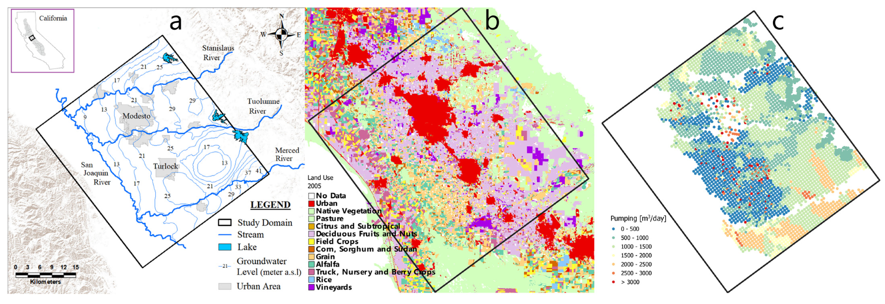
2.1. Description of the Study Area

The study site is the 2700 km2 agricultural region in the northeastern San Joaquin Valley straddling San Joaquin, Stanislaus, and Merced counties, California, and including eight different irrigation and water districts. It is constrained by the Sierra Nevada foothills to the northeast and the thalweg formed by the San Joaquin River to the southwest. The Stanislaus, Tuolumne, and Merced Rivers extend across the study area from northeast to southwest where they drain into the San Joaquin River (Figure 1). The ground surface slopes downward from the foothills with a gradient range of 1 m/km near the thalweg and up to 5 m/km near the foothills. The average annual rainfall is about 315 mm with a Mediterranean semi-arid climate. Rainfall is focused on the period from late fall to spring.
Agriculture, urban, and natural vegetation are three major land uses in the study area. More than 70% of the Modesto region is croplands, with almonds, walnuts, peaches, grapes, grain, corn, pasture, and alfalfa as the primary crops. More than 10% of the region is occupied by cities including Modesto and Turlock. The remainder is covered by natural vegetation, mostly grasslands near the foothills. Historical changes in agricultural land use have favored nitrate-demanding crop types (almond, corn; see Figure 2). Recharge rates, irrigation pumping rates, and nitrate leaching vary from crop to crop in the region and are also a function of soil type, management practices, and access to (less expensive) surface water.
The alluvial sediments of the eastern San Joaquin Valley form a heterogeneous semi-confined aquifer constrained locally by fine grained layers. The pre-development, natural pattern of groundwater recharge predominantly near the mountain front created a lateral northeast-to-southwest groundwater flow toward the major drainage of the Valley, the San Joaquin River [52]. Agricultural development and groundwater pumping in the 20th century added recharge in the form of irrigation return water (Figure 1b) and additional discharge in the form of irrigation pumping (Figure 1c and Figure S1) to the existing groundwater system, thus increasing the vertical component of groundwater flow [53,54]. The Corcoran Clay layer with maximum thickness of about 58 m is present throughout the western half of the study area at depths exceeding 26 m at its eastern boundary to 79 m near the San Joaquin River. This semi-confining layer separates the upper shallow aquifer from the lower confined aquifer. Nitrate contamination is a main concern in the study area, especially in the shallow aquifer. Details on the stratigraphy are provided in Section 2.4.

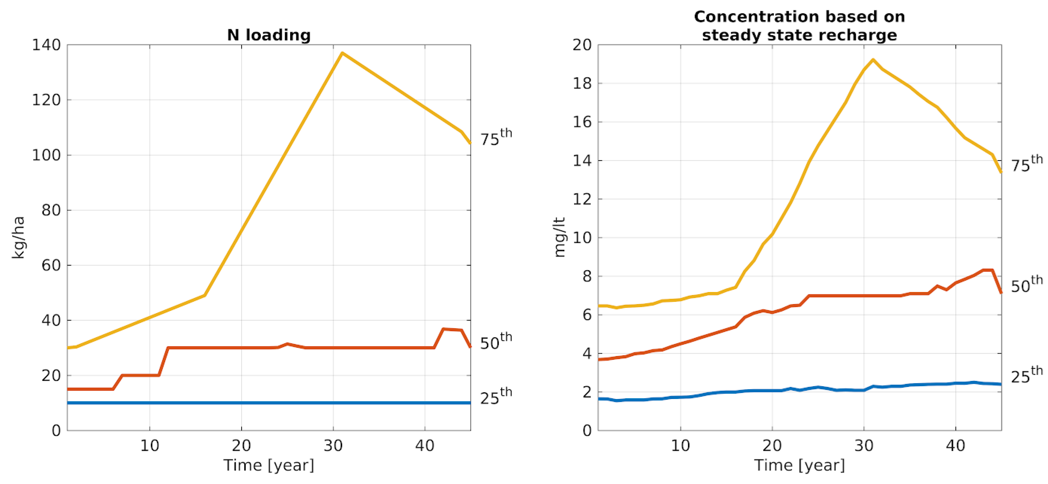
2.2. Nitrate Loading to Groundwater

Major sources of nitrate leaching to the water table within the agricultural and urban areas in the study region are the synthetic nitrogen fertilizers applied through crop irrigation, the vegetated urban landscapes, the leakage of sewer and septic systems, and applications of biosolids and animal manure. Harter et al. [55] estimated the average annual fluxes of nitrogen into and out of groundwater (nitrate load) for different land uses in the Central Valley, using a mass balance approach, for 6 fifteen-year periods from the mid-1940s to the mid-2000s (Table 1). The mass balance considers nitrogen in crop fertilizer, biosolids, manure, and urban wastes as input to the agricultural landscape. Nitrogen in harvested plants, atmospheric losses, runoff, and groundwater nitrate loading are outputs from the landscape, with the latter term used as the closing term (i.e., estimated using the mass balance).
Two groundwater nitrate loading scenarios were defined in this study to compare the performance of the full 3D finite difference ADE approach with the streamline-based transport technique. The first scenario is a “business-as-usual” (BAU) scenario, in which the estimated nitrate load from the mass balance method for 1960, 1975, 1990, and 2005 is linearly interpolated for intermediate years to obtain parcel-by-parcel nitrate loading from 1960 to 2005. The associated annual leaching concentration is allocated to corresponding modeling cells (Figure 3). The second scenario is a “best practice” scenario, in which the annual nitrate load applied under the BAU scenario is decreased by 25% for all years, representing a hypothetical agricultural Best Management Practice implementation in the region. In both scenarios, the aquifer is considered void of nitrate at the start of the simulation. Nitrate loading reduction may be due to a change in crop types or due to a change in nutrient management practices. Either approach can lead to less nitrogen fertilizer loading in the region.
A significant increase occurs in the nitrate loading time-series after 15 years from the start of the simulation period (Figure 3). After 30 years the loading input decreases due to improved practices [55]. In our simulation, we extended the loading beyond the 45th year by assuming a steady loading at the same rate as in the last year (year 45) for the remainder of a 200-year simulation period. The recharge concentration is a function of the recharge rates employed by the transient and steady-state flow models. The median recharge concentration ranged from 4 mg N/L to 8 mg N/L at the end of the 45 years. However, 25% of the study area receives input concentration that is above 6 mg N/L at the start of the simulation and above 20 mg N/L during the peak period. In this study, the vadose zone travel time is neglected. We assume that the contaminants leaving the root zone instantaneously arrive at the water table. We make this simplifying assumption here, because vadose zone travel time does not affect our groundwater-focused comparative analysis: the contaminant source loading at the water table is identical and consistent across the scenarios.

2.3. Numerical Methods: Mathematical Problem

The governing equation of transient groundwater flow in all three spatial dimensions in a saturated heterogeneous aquifer is as follows [56]:
x K x h x + y K y h y + z K z h z = S s h t
where K x , K y , and K z are saturated horizontal and vertical hydraulic conductivities at x, y, and z directions [L/T], h is hydraulic head [L], and S s is storage coefficient [L−1]. Numerical groundwater models usually solve (1) using a system of spatial and temporal discretization through which topographic data, aquifer parameters, boundary conditions, and sinks/sources of flow are represented. For steady-state groundwater flow, storage change (right-hand side of (1)) is zero.
The governing equation of groundwater transport of a non-reactive contaminant is expressed as follows [57]:
θ C t = . θ v C + . θ D C + q s C s
where θ is the porosity [unitless], C is the contaminant concentration [M/L3], v is the actual pore velocity (i.e., Darcy velocity divided by porosity) [L/T], D is the hydrodynamic dispersion tensor [L2/T], q s is the source (e.g., recharge or losing streams) or sink (e.g., discharging wells or gaining streams) volumetric flow rate per unit volume of aquifer [T−1], and C s is the source or sink contaminant concentration [M/L3].

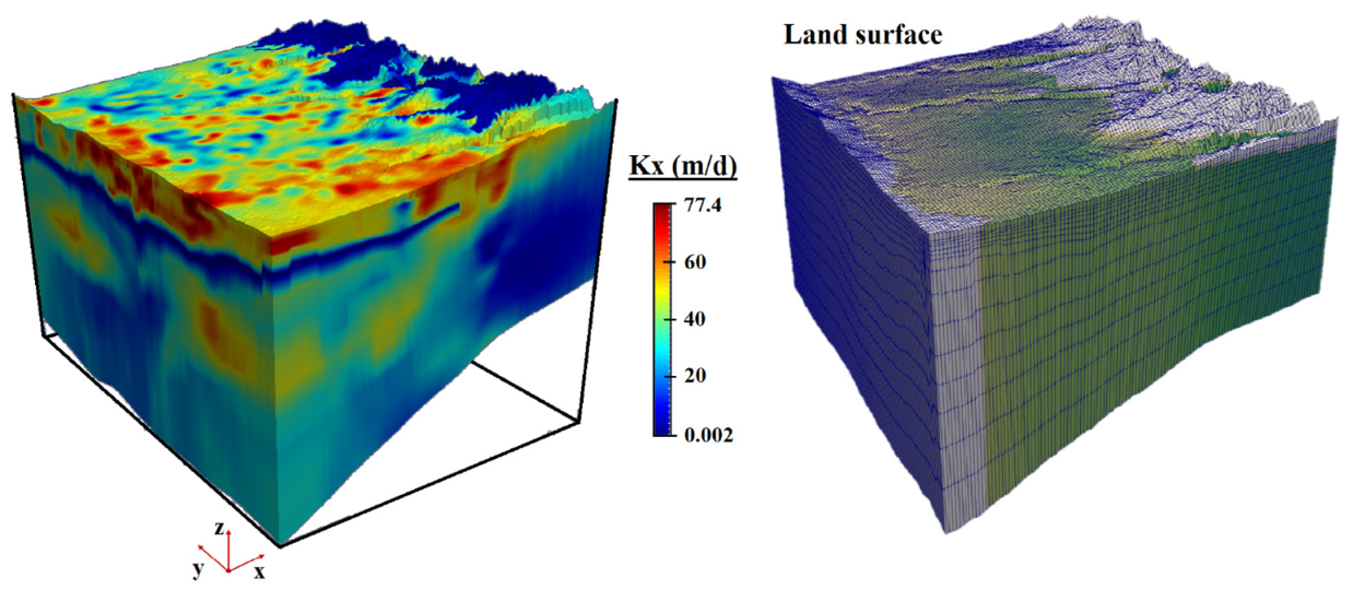
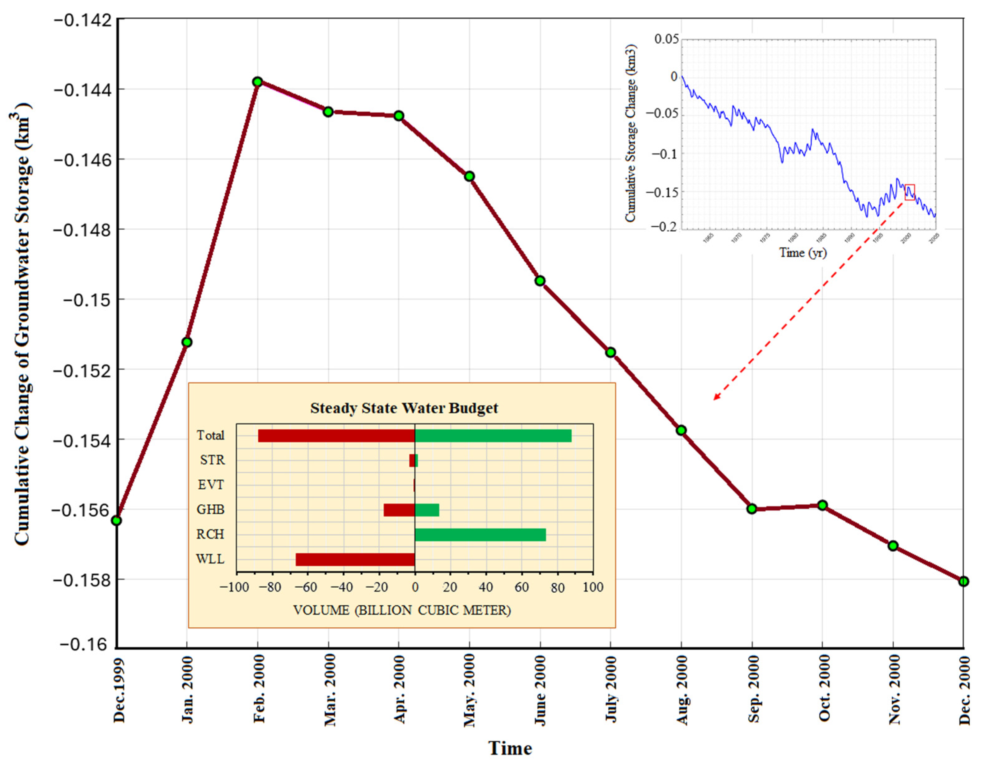
2.4. Numerical Methods: Transient and Steady-State Groundwater Flow Models

A transient groundwater flow model using the MODFLOW-2005 [56] platform was developed [16] building on a previously calibrated 45-year transient flow model of the Modesto study domain within the MODFLOW-OWHM platform [58,59]. Computed and user input boundary fluxes were imported to the MODFLOW-2005 platform to allow coupling with the MT3D transport model (not available for MODFLOW-OWHM, ibid.). Flow model cells are 400 m by 400 m horizontally with 153 rows and 137 columns and 16 model layers with thickness from 0.5 to 16 m above the Corcoran Clay and from 20 to 74 m below the Corcoran Clay. The top of the first layer represents the land surface. Layer thicknesses increase with depth.
No-flow boundary conditions were assigned to the northeastern side of the model along the Sierra Nevada foothills and most of the other lateral boundary conditions are classified as general-head based on the groundwater head data for the year 2000. The southwestern edge of the model is along the San Joaquin River which was simulated as a lateral general-head boundary condition. Cells west of the San Joaquin River are inactive for this model. Recharge enters the system in the model through the highest active cell and is defined by flow rate and concentration of nitrate. The study domain contains 3900 individual wells with different depths of screen categorized as shallow and deep pumping wells (Figure S1). Shallow wells extract groundwater from the upper aquifer above the Corcoran Clay layer.
Groundwater moves mainly from the northeastern foothill boundary toward the thalweg. The heterogeneous hydraulic conductivity distribution was calibrated through the original model [53] and ranges from 0.002 to 77.4 m/day for the horizontal hydraulic conductivity (Figure 4) and from 0.0018 to 19.38 m/day for the vertical hydraulic conductivity.
A steady-state groundwater flow model representing time-average hydrogeological stress conditions across the study area was developed in MODFLOW-2005 using water budget data for the year 2000 (“scheme6” in [39]). The choice was based on year 2000 being an average water year with stresses representative for the entire period. The ratio of storage change to the total pumped water is very small (1%, Figure 5), which makes the year 2000 an appropriate period for developing the steady-state model. The steady-state flow model requires a balanced water budget. To eliminate the 1% storage change in the transient model for application to the steady-state model, all outflows of the transient model water budget in the year 2000 were proportionally scaled by 1% to exactly match their inflows (Table S1). All other characteristics of the steady-state model (i.e., aquifer parameters and spatial discretization) were the same as the original transient flow model [39]. The same steady-state flow model boundary conditions and parameter distributions described here are also used with a finite element flow model [21,60], at higher resolution than the MODFLOW-2005 model, for coupling to the quasi-3D URF-based transport model (see Section 2.6).

2.5. Numerical Methods: Fully 3D ADE-Based Transport Model (MT3D)

A transient non-reactive transport model was developed using MT3D software [61] for use with both the transient and steady-state MODFLOW-2005 flow model implementations. Nitrate was the only solute considered in the system. The active transport model domain is the same as the active flow model domain. Land use (Section 2.2), recharge rates (m/d, Section 2.4), and nitrate load (kg/ha/yr, Section 2.2) distributions were known for every model cell for each year of the simulation. The recharge concentration of nitrate-nitrogen (mg N/L) was calculated for all upper active cells where recharge occurs into the groundwater model. Initial nitrate concentrations in 1960 were approximated as being negligibly small (zero) throughout the aquifer system [62]
The effective porosity distribution of the model was calculated from its correlation to percentage of coarse materials at each model cell ranging from 25 to 35% [18,63]. The longitudinal dispersivity ( a L ) was estimated as 11 m based on the scale of grid cells in the model [64]. Transverse horizontal dispersivity ( a T H ) and transverse vertical dispersivity ( a T V ) were 1.1 and 0.11 m, respectively ([65]). Initial concentration of nitrate was assumed to be zero everywhere in the system.
In this study, we are interested in the ensemble of concentration breakthrough curves (BTCs) at individual wells. The 3D ADE contaminant transport model estimates the concentration at every cell of the grid. However, the well screens span across multiple layers. We first calculate a single BTC for each well using the weighted average of the cell BTCs that intersect with each well. The contribution of each cell is assumed to be proportional to the horizontal hydraulic conductivity ([66]).

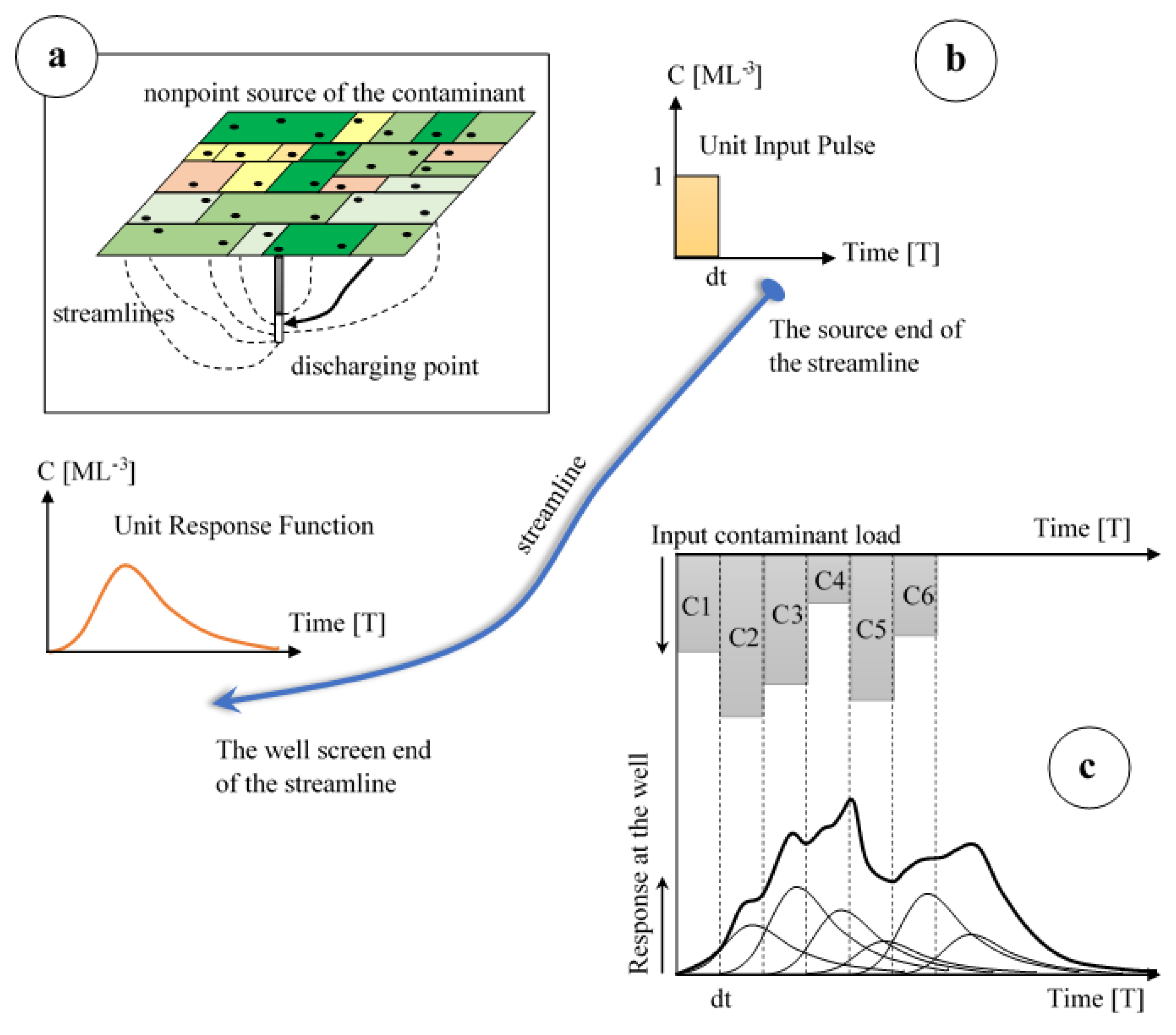
2.6. Numerical Methods: High-Resolution Flow with Quasi-3D URF-Based Transport Simulation

In the quasi-3D transport simulation framework (nonpoint source assessment tool “NPSAT”, [21]), the 3D transport process is decomposed into an ensemble of 1D transport subproblems. The NPSAT framework consists of the following steps (Figure 6):
  • Simulation of the groundwater flow field;
  • Backward particle tracking from the points of interest (compliance surfaces/well screens);
  • Streamline transport simulation with unit step/unit input loading to derive the streamline unit response functions (URFs);
  • Convolution of the URFs with a nitrate loading history scenario.
Steps 1–3 are implemented once (foundational). Step 4 can be repeated at exceedingly high computational efficiency for each (spatiotemporally heterogeneous) nitrate loading scenario of interest, which is, a critical attribute for decision-making support tools. For the steady-state flow simulation, we used a finite element approach with local refinement of the MODFLOW-2005 grid described above: cells that intersect with wells are split in half in each dimension, i.e., each MODFLOW well cell is divided into 8 cells [60]. This process was repeated recursively 8 times resulting in a minimum horizontal resolution around well screens of less than 2 m. Vertically, each well was discretized into a few hundred layers. The total number of degrees of freedom for the finite element solution of the steady-state flow equation is 32,127,378. While the parametrization of hydraulic properties and boundary conditions is identical to that described for the steady MODFLOW-2005 model, the location of the top boundary of the finite element mesh is explicitly simulated as the water table boundary ([60]): the position of the water table is obtained iteratively such that the hydraulic head of the top layer is equal to the node elevation of the top layer.

2.7. Statistical Analysis for Shallow and Deep Aquifer Model Comparison

We used standard correlation analysis to compare results between the different modeling approaches ([67]):
R = σ X Y σ X σ Y = i = 1 n ( x i μ x ) ( y i μ y ) n 1 / σ X σ Y
where R is the correlation coefficient, both X and Y are random variables, σ X Y is the covariance between X and Y, σ X is the standard deviation of X, σ Y is the standard deviation of Y, n is the number of the population in the random variables, x i is the associated value to each member of the population, and μ x and μ y are the mean values of the random variables X and Y, respectively. The ensemble of simulated wells is located with tops of well screens at depths ranging from 10 to 70 m deep below the water table. Statistical comparisons between model outcomes were grouped by the distance between the steady-state water table and the well’s screen top.

3. Results

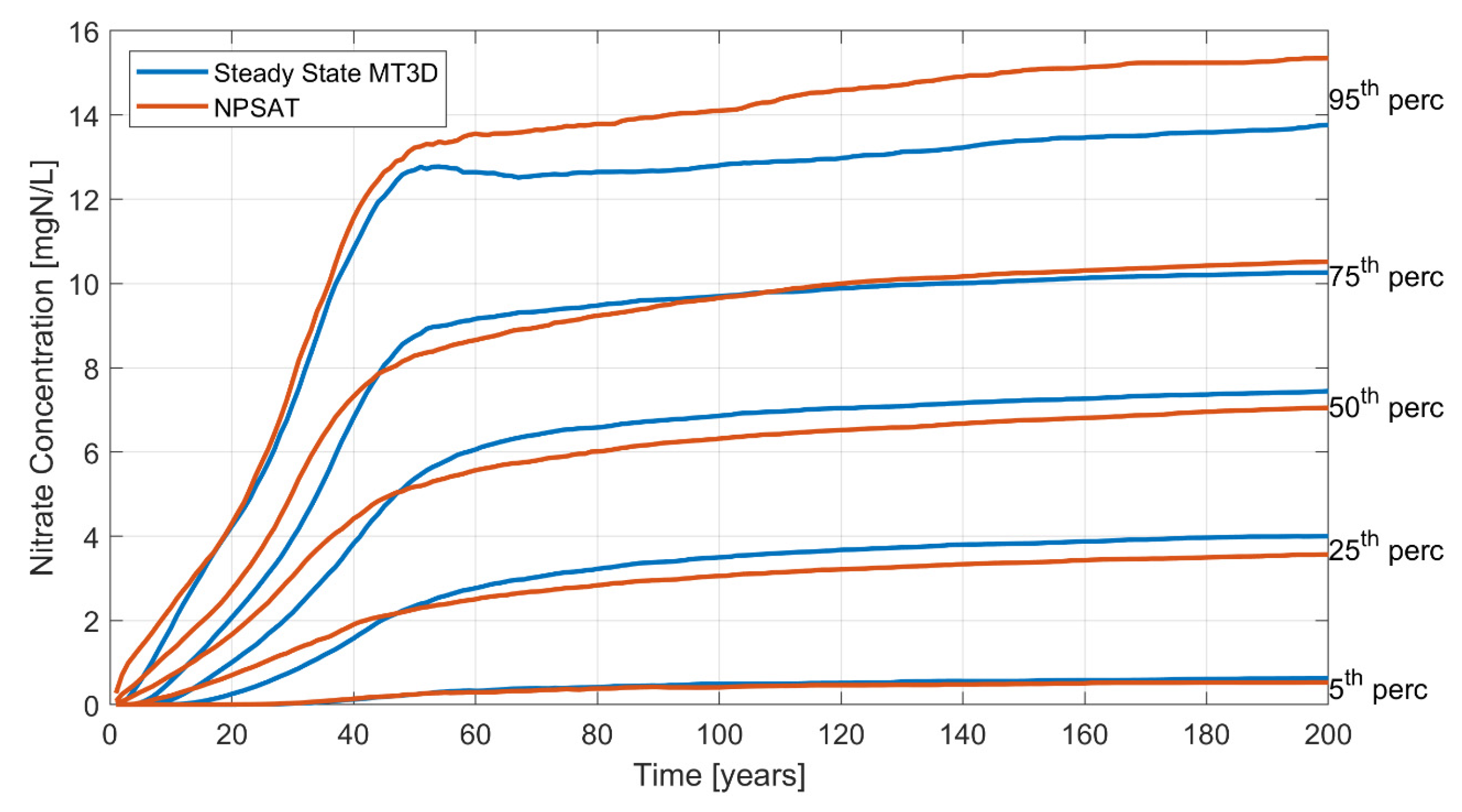
3.1. Business-as-Usual Simulations

Nitrogen loading from the landscape leads to low levels of nitrate arriving in some wells within less than five years. Across the ensemble of wells, all concentration quantiles increase monotonically over the simulation period. After rising for about 50 years, the worsening nitrate pollution begins to level off (Figure 7). However, a slight upward trend remains across all concentration quantiles over the remainder of the 200-year simulation period, indicating that many wells pump older groundwater and continue to be impacted by the initial 60-year rise in groundwater nitrate source loading, consistent, e.g., with the findings of [47]. A comparison of individual wells and ensemble simulated and measured nitrate concentrations over the historic period can be found for the fully 3D flow and transport model in [16,39]. The latter also provides a detailed comparison of the steady-state flow approximation results with fully transient flow and transport simulations.
For the nitrate (as nitrogen) concentration percentiles across the ensemble of study area wells, the steady-state flow and URF-based transport model, NPSAT, generally follows a similar predication pattern to the fully 3D, lower-spatial-resolution transport model (“MT3D”). Over almost the entire simulation period, the highest concentrations (95th percentile) have the largest prediction discrepancy: from t = 10 years onward, they range from 5 to 15% higher with NPSAT, compared to MT3D, showing 15 mg/L instead of 13.5 mg/L at t = 200 years. For the 70th percentile (not shown in the figure), the two models predict almost identical concentration at the end of the simulation period. But the discrepancy for the 80th, 90th, and 95th percentiles becomes 3.7, 7.8, and 10%, respectively.
For the same time period (t = 10 years to 200 years), generally smaller discrepancies (<1 mg/L) exist for lower percentiles. These discrepancies are much smaller than the range of concentration quantiles observed, from less than 1 mg/L for the 5th percentile to over 13 mg/L for the 95th percentile, indicating that both methods capture similar overall concentration dynamics across the ensemble of wells of interest.
The discrepancy between median predictions at t > 100 is less than 10%, with NPSAT predicting higher concentrations before year 45 and lower concentrations than MT3D after this time. Similarly, the NPSAT model predicts the lower percentiles of breakthrough curves (i.e., 5th and 25th percentiles) initially at higher concentrations than MT3D but at lower concentrations than MT3D for t > 50 years (with differences less than 0.5 mg/L).
The relatively largest discrepancies are observed during the initial 10-year simulation period: NPSAT generates much earlier arrival of nitrate in some wells than MT3D, leading all concentration percentiles to be several-fold higher in NPSAT over the first one to two decades. However, absolute differences between NPSAT and MT3D during this early period are less than 2 mg/L (20% of the MCL concentration for nitrate-N).
For the most critical initial 45-year period, we also compare the percentile breakthrough curve results of the two steady-state flow-based transport simulations with those of the transient flow-based transport model [39]. Overall, the steady-state representations (both NPSAT and MT3D) overestimate the concentrations obtained from the transient simulation by as much as 1.7 mg/L for NPSAT and 0.7 mg/L for MT3D (Figure 8). Across percentiles, similar differences in breakthrough curve dynamics are observed between NPSAT and MT3D and between steady-state flow and transient flow simulations (Figure 8). Transient simulations lead to a lower nitrate concentration in wells, with the relative difference being the largest for the lowest concentration percentile (5th), but with absolute differences of less than 0.1 mg/L. Differences between the transient and steady-state-flow-based MT3D simulations have been further discussed by [39]. They are thought to result from the lack of some dilution effects introduced by the transient flow system (with most groundwater pumping occurring only during late spring, summer, and early fall).

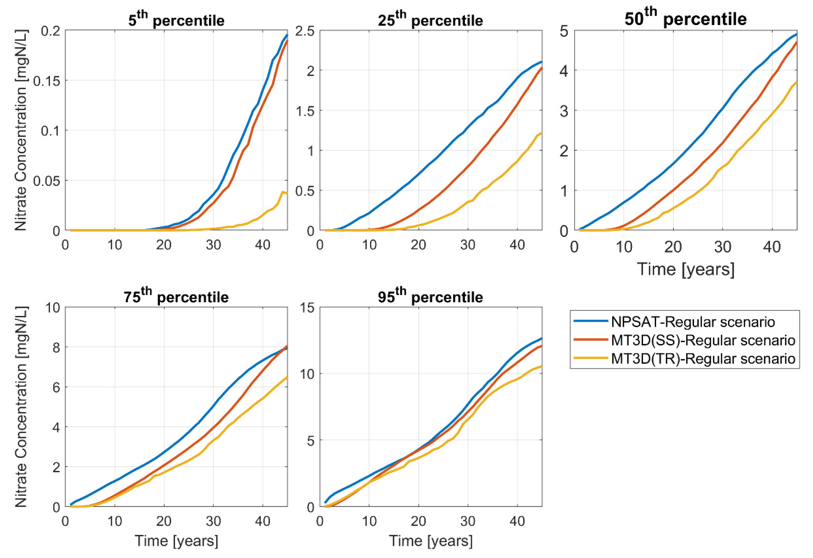
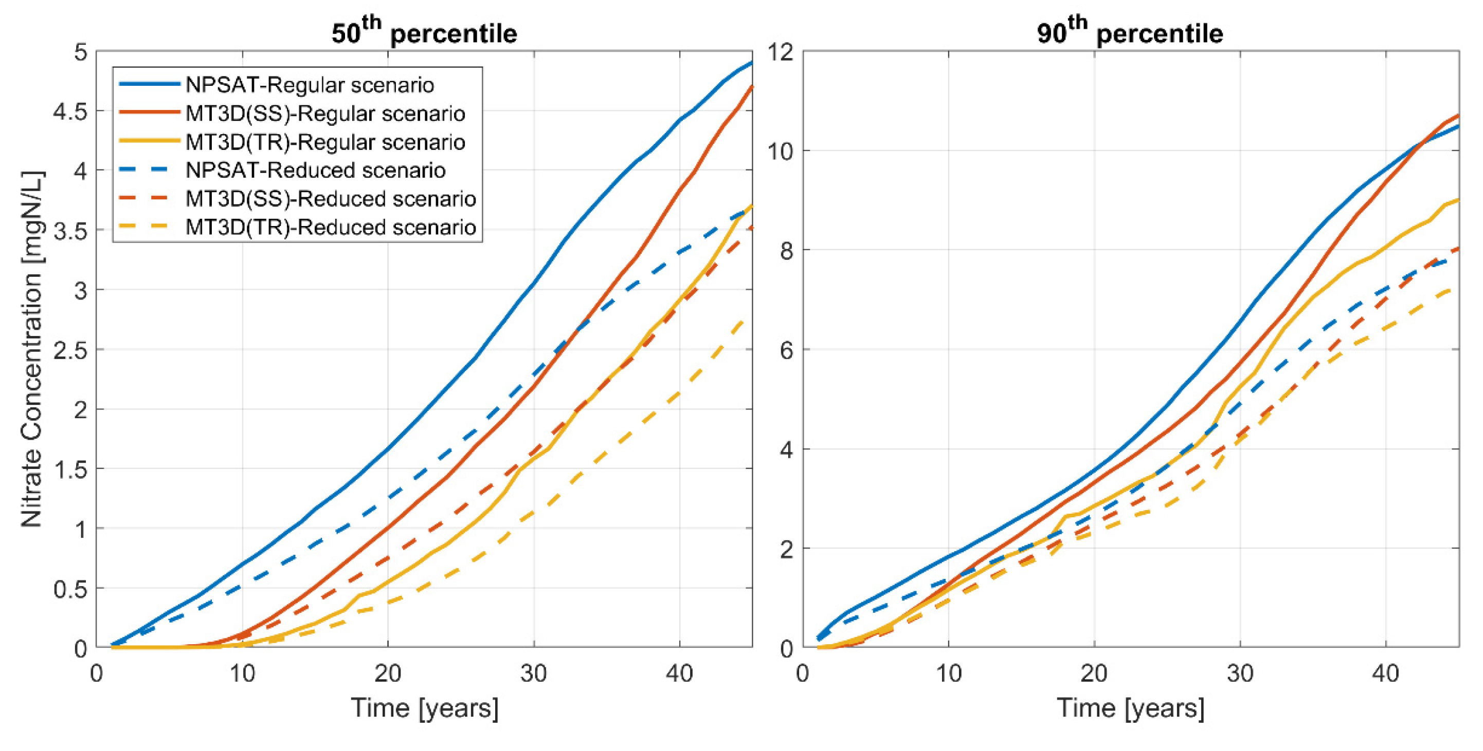
3.2. Predicting Relative Future Changes

Stakeholders’ and decision-makers’ primary use of models as a decision-support tool involves evaluating future changes in nitrate concentration resulting from alternative reduced loading scenarios on a regional scale. For the reduced loading scenario tested here, all three models produced 25% lower nitrate concentrations at the targeted wells, showing the potential improvement that may be achieved by reducing nitrate loading in recharge (Figure 9). While the absolute values are different (as described above), the relative attenuation of nitrate achieved in wells is predicted to be identical between all three models. Hence, the application of the steady-state flow-based transport simulation is particularly suitable for predicting relative (rather than absolute) changes in future scenario analyses.

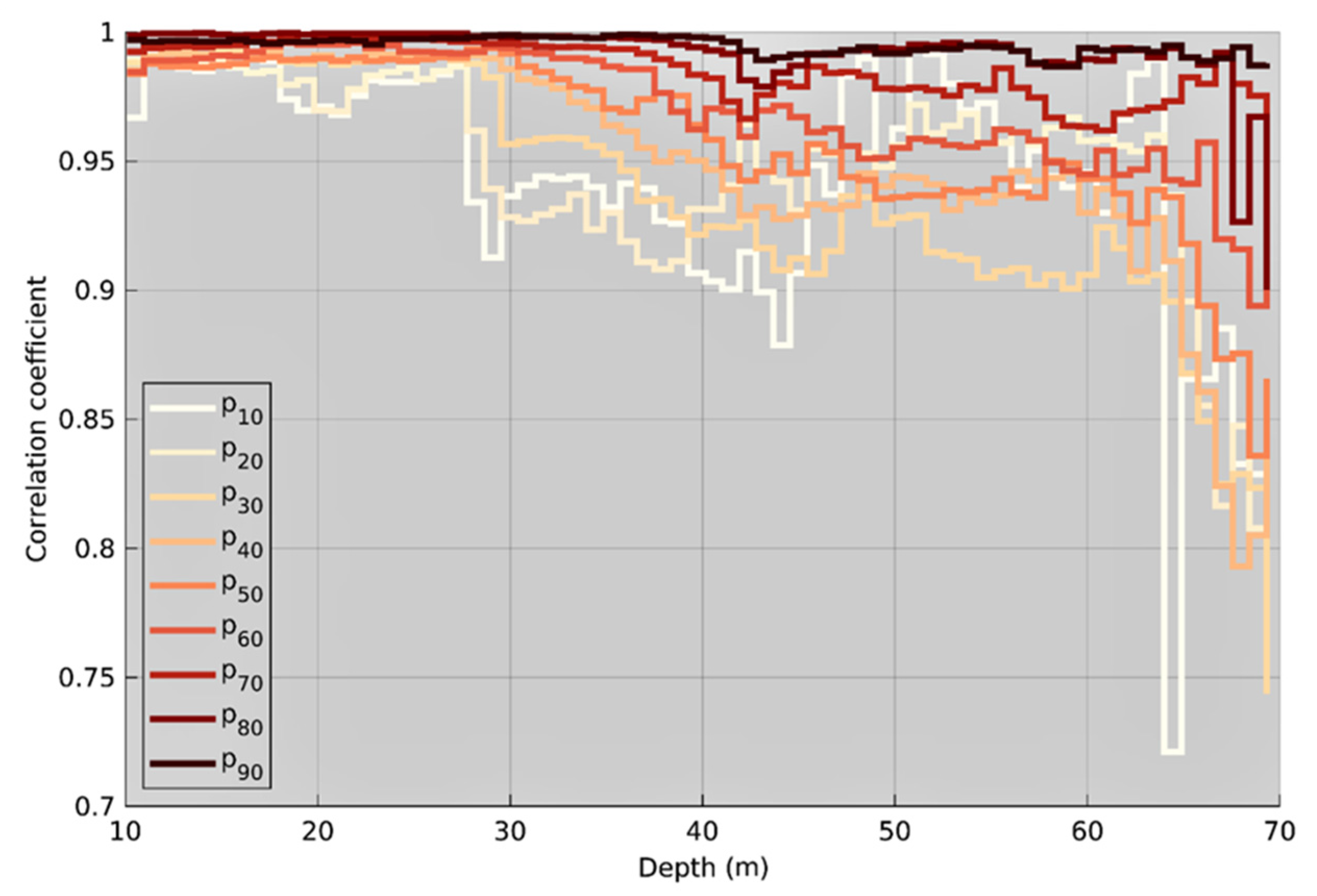
3.3. Depth-Dependent Correlation of NPSAT and MT3D Results

The calculated well concentrations at the end of the simulation period are highly correlated between NPSAT and MT3D simulations (Figure 10). When considering depth, we find that the correlation coefficient (Figure 10) is highest at a shallow depth (nearly 1) but decreases for a larger depth (to about 0.7). Hence, agreement between the two models is stronger in shallow aquifers and gradually declines through deeper zones. This is the result of larger differences in travel path length between NPSAT and MT3D as depth increases. It can also be attributed to the source area of deeper wells often being larger than the source area of shallow wells due to the often longer screen size [47].

4. Discussion

The differences between the steady-state-flow-based NPSAT and MT3D simulations result primarily from the different discretization, especially around the well screens (less than 10 m in NPSAT but 400 m in MT3D) and from differences in accounting for transverse dispersion—no transverse dispersion in NPSAT and small transverse dispersion in MT3D. Accounting for transverse dispersion, given the spatial distribution of the source signal and general shape of the ensemble percentile breakthrough curves, this affects the breakthrough curve due to the lateral mass exchange between water flow paths. However, since the source is laterally extensive, the influence of transverse dispersion is thought to be small, even in high-resolution models. Henri and Harter [47] showed that mixing across the compliance surface (here: well screen) dominates nitrate breakthrough dynamics relative to dispersion. The dispersion signal itself is dominated by longitudinal dispersion, with transverse dispersion contributing much less to the breakthrough dynamics than longitudinal dispersion. Macro-scale transverse dispersion due to aquifer heterogeneity is taken into account identically between the two approaches, through corresponding parametrization of the hydraulic conductivity [34,68,69,70].
The main contribution to the difference between NPSAT and MT3D therefore originates from differences in discretization. The nearly 2-order-of-magnitude coarser discretization around wells in MT3D limits the ability to simulate the converging flow field around wells. This leads, in MT3D, to narrower and more elongated source areas [23], which in turn may explain the delay in breakthrough: the finer lateral and vertical discretization around well screens in NPSAT would more accurately capture the convergent flow field around pumping wells and the accelerated downward gradient above the well screen, creating some shorter flow paths (shorter travel times) near the top of the well screen. Early travel times of nitrate have been observed, e.g., by [71,72,73]. In these studies, the residence time distributions of nitrate particles on the local and sub-regional scales are examined in the same way as here using analytical and particle tracking numerical models.
Given NPSAT’s higher resolution, longer flow paths (longer travel times) would be observed, relative to MT3D, at the downstream side of the well screen and near the bottom of the well screen. The wider range of travel path lengths and, hence, wider spread in travel time explains the wider range of concentrations in NPSAT. It also suggests that the NPSAT solution is more accurate than the MT3D solution, due to the finer discretization and despite the lack of simulating transverse dispersion.
Additionally, transverse dispersivity is very small (1.1 m) compared to the discretization in MT3D (400 m). Not only are the effects of transverse dispersivity on this grid scale very small, they are also numerically difficult to capture without significant numerical dispersion (numerically induced dispersion). The MT3D solution has limited capacity to accurately solve very small subgrid-scale transverse dispersion. Heterogeneity-induced, macro-scale transverse dispersion is captured equally by both models due to the shared underlying heterogeneous hydraulic conductivity distribution.
While there are small but significant differences between NPSAT and MT3D, and somewhat more so between NPSAT and the fully transient flow MT3D, all three numerical approaches provide similar statistical results across the ensemble of wells. In practice, the differences in the statistical distribution of nitrate concentrations between the three simulation tools appear sufficiently small to argue that any of these approaches would provide similar orientation to decision-making processes.

Computational Efficiency of the URF-Based Transport Simulator

The study of basin-wide consequences of land use management practices for improving the quality of groundwater resources requires using practical and computational efficient modeling tools to perform long-term analysis of alternative future scenarios [74,75]. Fully 3D physical-based models have been the scientific standard to simulate groundwater flow and advective–dispersive transport in groundwater. However, the computational cost and parameter uncertainty of detailed processes in such models make them “impracticable” for basin-scale problems [76]. Carle et al. [34] demonstrated that highly heterogeneous basin-scale transport models can indeed be implemented through the use of advanced, massively parallel software and hardware architectures, but there are obvious benefits to attempting to achieve similar or adequate results with simpler and faster models.
A key feature of using a steady-state flow solution to define advection in the transport equation is that it allows the development of URFs and the use of a convolution to solve each of many (hundreds, thousands or more) individual spatio-temporally distributed pollution source loading scenarios at very high computational speed. The total run time of the land use change scenario in the current work was 90 min for the fully 3D steady flow-based transient MT3D simulation. The prediction simulation time for the quasi-3D URF-based streamline model is in the order of a few seconds, a three-order-of-magnitude speed-up. Hence, the streamline approach offers opportunities for simulating a large number of individual future loading scenarios after some computational investment into preparing a high-resolution flow solution. The approach is useful for web-based scenario simulators and as a decision-support tool.
For management scenarios that examine significant changes in the flow conditions, e.g., managed aquifer recharge (MAR) projects, both modeling approaches require simulation of flow and transport. In the 3D ADE approach, it is possible to simulate the flow changes using a single run, which would correspond to a single contaminant/land use management scenario, while in the URF-based method, a separate steady-state approximation would be needed. However, it can be used to simulate multiple contaminant management scenarios that correspond to similar flow conditions.

5. Conclusions

In this study, we compare two frameworks for the simulation of nonpoint source (diffuse) pollution in large agricultural groundwater basins: the URF-based streamline transport framework proposed by [21] was compared with the general 3D advection–dispersion simulation framework focusing on the breakthrough curves of the nonpoint source contaminant at discharging wells. We assessed the two major underlying assumptions of the URF-based method: (i) groundwater flow is well approximated by steady-state conditions and (ii) the effect of transverse dispersivity is negligible. The investigation of these assumptions focused on long-term scenario analysis applications. A fully three-dimensional transient heterogeneous (at the scale of 400 by 400 m2 cells) groundwater flow and transport model was used as the basis of a comparison of results. In addition, a steady-state version of the transient model was developed using both the fully 3D ADE and the URF-based streamline approach. The following conclusions can be drawn from the work presented:
  • Albeit lacking transverse dispersion, the URF-based method shows very good agreement with the 3D ADE solution, when both are based on a steady-state flow field (maximum discrepancies are 10%, observed for the most contaminated fraction of wells).
  • Similarly, the 3D ADE solution based on a significantly coarser grid around wells than the URF-based framework proposed has an only slightly reduced spread of concentration percentiles across the ensemble of wells, relative to the URF-based framework.
  • Using the steady-state approximation of the cyclically transient flow field yields similar disagreements to the 3D-ADE-based solution with the transient flow field, whether using the 3D-ADE- or the URF-based transport model. The 3D-ADE-based solution for a steady flow field is closer to that for a transient flow field than the URF-based solution, possibly due to the lack of difference in the discretization of the flow-field between the 3-ADE solutions for steady and transient flow.
  • The URF-based transport solution in the case study (evaluation of nitrate BTCs at 3900 wells over a 45-year simulation period) maintains at least three-order-of-magnitude gains in computational efficiency for nitrate loading scenario evaluation.
  • The URF-based transport solution is applicable to a wide range of solutes as it retains the ability to also account for reactive transport of contaminants or tracers subject to retardation (sorption) and/or first-order degradation.
  • Model agreement was shown to depend on the vertical location of the well screen. The correlation of the predictions between the models is higher between the URF-based and 3D ADE models for the shallow wells. For deep wells, differences between travel path length in the high-resolution, URF-based framework and the lower-resolution 3D ADE framework lead to smaller spread of travel time in the latter approach.
  • The results suggest that diffusion, transverse dispersion, and cyclical transiency of the velocity field have relatively small effects on the ensemble statistical outcome of contaminant concentration across a large group of CSs (wells, stream reaches) in a region with diverse, contiguous nonpoint sources of evolving strength. The observed variability of concentration between CSs is predominantly driven by (i) the variability among source concentrations emitted across the landscape to the water table and (ii) the variability across CSs with respect to the number and diversity of sources mixed into the waters of an individual CS (e.g., within a well screen).
  • We are currently conducting additional research to more rigorously compare the relative contributions of in-well (within CS) mixing, aquifer heterogeneity (macro-dispersion), mechanical dispersion, and diffusion to nonpoint source pollutant/solute transport in aquifer systems (e.g., [44,47]).
  • The efficiency of the URF-based approach makes it appropriate for decision-makers and stakeholders. However, future research is needed to identify suitable methods and tools to incorporate the modeling framework into a suitable tool, e.g., web-based or server applications that can be used by policy makers and planners.
In this paper, we focused on the comparison between the different modeling approaches for both flow (steady-state versus transient) and transport (quasi-3D without transverse dispersion versus full = 3D). Future research is needed to compare the predictions of the URF-based approach against measured diffuse pollution such as nitrate and salinity. In addition, the quasi-3D approach can be validated against measured age tracer concentrations, another diffuse source of groundwater solute tracers.

Supplementary Materials

The following supporting information can be downloaded at https://figshare.com/s/303a0413cfd9e6278ac4 (accessed on 9 January 2025): Table S1: Cumulative volumetric water budget comparison of the study area flow platforms; https://doi.org/10.6084/m9.figshare.28182695 (accessed on 9 January 2025); Figure S1: Modesto well depth.

Author Contributions

Conceptualization, G.K., M.B., and T.H.; methodology, G.K., M.B., and T.H.; writing—original draft preparation, M.B. and G.K.; writing—review and editing, G.K., M.B., and T.H.; visualization, M.B. and G.K.; supervision, T.H.; project administration, T.H.; funding acquisition, T.H. All authors have read and agreed to the published version of the manuscript.

Funding

This research was funded by the California State Water Resources Control Board, grant agreement no. 19-051-250-2, USDA NRCS, grant agreement NR233A750023C047, and USDA NIFA Award 2021-68012-35914.

Data Availability Statement

Data available upon request.

Acknowledgments

We would like to thank Steven Phillips for kindly providing us with the MODFLOW-OWHM transient model of the study area. We also express our appreciation to Graham Fogg, University of California Davis, for his valuable comments to improve this paper.

Conflicts of Interest

The authors declare no conflicts of interest.

References

  1. Zhou, Y.; Khu, S.-T.; Xi, B.; Su, J.; Hao, F.; Wu, J.; Huo, S. Status and Challenges of Water Pollution Problems in China: Learning from the European Experience. Environ. Earth Sci. 2014, 72, 1243–1254. [Google Scholar] [CrossRef]
  2. Adimalla, N.; Qian, H. Groundwater Quality Evaluation Using Water Quality Index (WQI) for Drinking Purposes and Human Health Risk (HHR) Assessment in an Agricultural Region of Nanganur, South India. Ecotoxicol. Environ. Saf. 2019, 176, 153–161. [Google Scholar] [CrossRef] [PubMed]
  3. Armour, J.D.; Nelson, P.N.; Daniells, J.W.; Rasiah, V.; Inman-Bamber, N.G. Nitrogen Leaching from the Root Zone of Sugarcane and Bananas in the Humid Tropics of Australia. Agric. Ecosyst. Environ. 2013, 180, 68–78. [Google Scholar] [CrossRef]
  4. Biggs, J.S.; Thorburn, P.J.; Crimp, S.; Masters, B.; Attard, S.J. Interactions between Climate Change and Sugarcane Management Systems for Improving Water Quality Leaving Farms in the Mackay Whitsunday Region, Australia. Agric. Ecosyst. Environ. 2013, 180, 79–89. [Google Scholar] [CrossRef]
  5. Van Grieken, M.E.; Roebeling, P.C.; Bohnet, I.C.; Whitten, S.M.; Webster, A.J.; Poggio, M.; Pannell, D. Adoption of Agricultural Management for Great Barrier Reef Water Quality Improvement in Heterogeneous Farming Communities. Agric. Syst. 2019, 170, 1–8. [Google Scholar] [CrossRef]
  6. Lockhart, K.M.; King, A.M.; Harter, T. Identifying sources of groundwater nitrate contamination in a large alluvial groundwater basin with highly diversified intensive agricultural production. J. Contam. Hydrol. 2013, 151, 140–154. [Google Scholar] [CrossRef]
  7. Yang, A.L.; Raghuram, N.; Adhya, T.K.; Porter, S.D.; Panda, A.N.; Kaushik, H.; Jayaweera, A.; Nissanka, S.P.; Anik, A.R.; Shifa, S.; et al. Policies to Combat Nitrogen Pollution in South Asia: Gaps and Opportunities. Environ. Res. Lett. 2022, 17, 025007. [Google Scholar] [CrossRef]
  8. Hansen, B.; Thorling, L.; Schullehner, J.; Termansen, M.; Dalgaard, T. Groundwater Nitrate Response to Sustainable Nitrogen Management. Sci. Rep. 2017, 7, 8566. [Google Scholar] [CrossRef]
  9. Platjouw, F.M.; Nesheim, I.; Enge, C. Policy Coherence for the Protection of Water Resources against Agricultural Pollution in the EU and Norway. Rev. Eur. Comp. Int. Environ. Law 2023, 32, 485–500. [Google Scholar] [CrossRef]
  10. Velthof, G.L.; Lesschen, J.P.; Webb, J.; Pietrzak, S.; Miatkowski, Z.; Pinto, M.; Kros, J.; Oenema, O. The Impact of the Nitrates Directive on Nitrogen Emissions from Agriculture in the EU-27 during 2000–2008. Sci. Total Environ. 2014, 468–469, 1225–1233. [Google Scholar] [CrossRef]
  11. Kallis, G.; Butler, D. The EU Water Framework Directive: Measures and Implications. Water Policy 2001, 3, 125–142. [Google Scholar] [CrossRef]
  12. California State of Sustainable Groundwater Management Act (SGMA). Available online: https://water.ca.gov/Programs/Groundwater-Management/SGMA-Groundwater-Management (accessed on 17 February 2025).
  13. Lubell, M.; Blomquist, W.; Beutler, L. Sustainable Groundwater Management in California: A Grand Experiment in Environmental Governance. Soc. Nat. Resour. 2020, 33, 1447–1467. [Google Scholar] [CrossRef]
  14. Salt Program. CV SALTS. Available online: https://www.cvsalinity.org/ (accessed on 17 February 2025).
  15. Quinn, N.W.T.; Oster, J.D. Innovations in Sustainable Groundwater and Salinity Management in California’s San Joaquin Valley. Sustainability 2021, 13, 6658. [Google Scholar] [CrossRef]
  16. Bastani, M.; Harter, T. Source Area Management Practices as Remediation Tool to Address Groundwater Nitrate Pollution in Drinking Supply Wells. J. Contam. Hydrol. 2019, 226, 103521. [Google Scholar] [CrossRef] [PubMed]
  17. McMahon, P.B.; Böhlke, J.K.; Kauffman, L.J.; Kipp, K.L.; Landon, M.K.; Crandall, C.A.; Burow, K.R.; Brown, C.J. Source and Transport Controls on the Movement of Nitrate to Public Supply Wells in Selected Principal Aquifers of the United States. Water Resour. Res. 2008, 44, W04401. [Google Scholar] [CrossRef]
  18. McMahon, P.B.; Burow, K.R.; Kauffman, L.J.; Eberts, S.M.; Böhlke, J.K.; Gurdak, J.J. Simulated Response of Water Quality in Public Supply Wells to Land Use Change. Water Resour. Res. 2008, 44, W00A06. [Google Scholar] [CrossRef]
  19. Kuai, P.; Li, W.; Liu, N. Evaluating the Effects of Land Use Planning for Non-Point Source Pollution Based on a System Dynamics Approach in China. PLoS ONE 2015, 10, e0135572. [Google Scholar] [CrossRef]
  20. Zhang, H.; Hiscock, K.M. Modelling Response of Groundwater Nitrate Concentration in Public Supply Wells to Land-Use Change. Q. J. Eng. Geol. Hydrogeol. 2016, 49, 170–182. [Google Scholar] [CrossRef]
  21. Kourakos, G.; Klein, F.; Cortis, A.; Harter, T. A Groundwater Nonpoint Source Pollution Modeling Framework to Evaluate Long-Term Dynamics of Pollutant Exceedance Probabilities in Wells and Other Discharge Locations. Water Resour. Res. 2012, 48, W00L13. [Google Scholar] [CrossRef]
  22. Hansen, B.; Dalgaard, T.; Thorling, L.; Sørensen, B.; Erlandsen, M. Regional Analysis of Groundwater Nitrate Concentrations and Trends in Denmark in Regard to Agricultural Influence. Biogeosciences 2012, 9, 3277–3286. [Google Scholar] [CrossRef]
  23. Boyle, D.; King, A.; Kourakos, G.; Lockhart, K.; Mayzelle, M.; Fogg, G.; Harter, T. Groundwater Nitrate Occurrence. Technical Report 4 in: Addressing Nitrate in California’s Drinking Water with a Focus on Tulare Lake Basin and Salinas Valley Groundwater; Report for the State Water Resources Control Board Report to the Legislature; Center for Watershed Sciences, University of California: Davis, CA, USA, 2012. [Google Scholar]
  24. Turkeltaub, T.; Kurtzman, D.; Dahan, O. Real-Time Monitoring of Nitrate Transport in the Deep Vadose Zone under a Crop Field—Implications for Groundwater Protection. Hydrol. Earth Syst. Sci. 2016, 20, 3099–3108. [Google Scholar] [CrossRef]
  25. Ransom, K.M.; Nolan, B.T.A.; Traum, J.; Faunt, C.C.; Bell, A.M.; Gronberg, J.A.M.; Wheeler, D.C.Z.; Rosecrans, C.; Jurgens, B.; Schwarz, G.E.; et al. A Hybrid Machine Learning Model to Predict and Visualize Nitrate Concentration throughout the Central Valley Aquifer, California, USA. Sci. Total Environ. 2017, 601–602, 1160–1172. [Google Scholar] [CrossRef] [PubMed]
  26. Rosecrans, C.Z.; Nolan, B.T.; Gronberg, J.M. Prediction and Visualization of Redox Conditions in the Groundwater of Central Valley, California. J. Hydrol. 2017, 546, 341–356. [Google Scholar] [CrossRef]
  27. Milnes, E.; Perrochet, P. Simultaneous Identification of a Single Pollution Point-Source Location and Contamination Time under Known Flow Field Conditions. Adv. Water Resour. 2007, 30, 2439–2446. [Google Scholar] [CrossRef]
  28. Zhou, Y.; Jiang, Y.; An, D.; Ma, Z.; Xi, B.; Yang, Y.; Li, M.; Hao, F.; Lian, X. Simulation on Forecast and Control for Groundwater Contamination of Hazardous Waste Landfill. Environ. Earth Sci. 2014, 72, 4097–4104. [Google Scholar] [CrossRef]
  29. Abd-Elaty, I.; Zelenakova, M.; Straface, S.; Vranayová, Z.; Abu-hashim, M. Integrated Modelling for Groundwater Contamination from Polluted Streams Using New Protection Process Techniques. Water 2019, 11, 2321. [Google Scholar] [CrossRef]
  30. Colman, J.A.; Masterson, J.P. Transient Simulations of Nitrogen Load for a Coastal Aquifer and Embayment, Cape Cod, MA. Environ. Sci. Technol. 2008, 42, 207–213. [Google Scholar] [CrossRef]
  31. Yager, R.M.; Heywood, C.E. Simulation of the Effects of Seasonally Varying Pumping on Intraborehole Flow and the Vulnerability of Public-Supply Wells to Contamination. Groundwater 2014, 52, 40–52. [Google Scholar] [CrossRef]
  32. Bexfield, L.M.; Jurgens, B.C. Effects of Seasonal Operation on the Quality of Water Produced by Public-Supply Wells. Groundwater 2014, 52, 10–24. [Google Scholar] [CrossRef]
  33. Hiscock, K.; Lovett, A.; Saich, A.; Dockerty, T.; Johnson, P.; Sandhu, C.; Sünnenberg, G.; Appleton, K.; Harris, B.; Greaves, J. Modelling Land-Use Scenarios to Reduce Groundwater Nitrate Pollution: The European Water4All Project. Q. J. Eng. Geol. Hydrogeol. 2007, 40, 417–434. [Google Scholar] [CrossRef]
  34. Carle, S.F.; Esser, B.K.; Moran, J.E. High-Resolution Simulation of Basin-Scale Nitrate Transport Considering Aquifer System Heterogeneity. Geosphere 2006, 2, 195–209. [Google Scholar] [CrossRef]
  35. Lin, L.; Yang, J.-Z.; Zhang, B.; Zhu, Y. A Simplified Numerical Model of 3-D Groundwater and Solute Transport at Large Scale Area. J. Hydrodyn. 2010, 22, 319–328. [Google Scholar] [CrossRef]
  36. Prommer, H.; Barry, D.A.; Davis, G.B. Modelling of Physical and Reactive Processes during Biodegradation of a Hydrocarbon Plume under Transient Groundwater Flow Conditions. J. Contam. Hydrol. 2002, 59, 113–131. [Google Scholar] [CrossRef] [PubMed]
  37. Yin, Y.; Sykes, J.F.; Normani, S.D. Impacts of Spatial and Temporal Recharge on Field-Scale Contaminant Transport Model Calibration. J. Hydrol. 2015, 527, 77–87. [Google Scholar] [CrossRef]
  38. Zheng, C.; Wang, P.P. A Field Demonstration of the Simulation Optimization Approach for Remediation System Design. Groundwater 2002, 40, 258–266. [Google Scholar] [CrossRef]
  39. Bastani, M.; Harter, T. Effects of Upscaling Temporal Resolution of Groundwater Flow and Transport Boundary Conditions on the Performance of Nitrate-Transport Models at the Regional Management Scale. Hydrogeol. J. 2020, 28, 1299–1322. [Google Scholar] [CrossRef]
  40. Martin, J.C.; Wegner, R.E. Numerical Solution of Multiphase, Two-Dimensional Incompressible Flow Using Stream-Tube Relationships. Soc. Pet. Eng. J. 1979, 19, 313–323. [Google Scholar] [CrossRef]
  41. Matringe, S.F.; Juanes, R.; Tchelepi, H.A. Robust Streamline Tracing for the Simulation of Porous Media Flow on General Triangular and Quadrilateral Grids. J. Comput. Phys. 2006, 219, 992–1012. [Google Scholar] [CrossRef]
  42. Robinson, B.A.; Dash, Z.V.; Srinivasan, G. A Particle Tracking Transport Method for the Simulation of Resident and Flux-Averaged Concentration of Solute Plumes in Groundwater Models. Comput. Geosci. 2010, 14, 779–792. [Google Scholar] [CrossRef]
  43. Valocchi, A.J.; Herrera, P.; Viswanathan, H. Incorporating Transverse Mixing into Streamline-Based Simulation of Transport in Heterogeneous Aquifers. In Groundwater Quality Modeling and Management Under Uncertainty; American Society of Civil Engineers: Reston, VA, USA, 2003; pp. 294–304. [Google Scholar] [CrossRef]
  44. Henri, C.V.; Harter, T. Denitrification in Heterogeneous Aquifers: Relevance of Spatial Variability and Performance of Homogenized Parameters. Adv. Water Resour. 2022, 164, 104168. [Google Scholar] [CrossRef]
  45. Kourakos, G.; Harter, T. Vectorized Simulation of Groundwater Flow and Streamline Transport. Environ. Model. Softw. 2014, 52, 207–221. [Google Scholar] [CrossRef]
  46. Kourakos, G.; Harter, T. Parallel Simulation of Groundwater Non-Point Source Pollution Using Algebraic Multigrid Preconditioners. Comput. Geosci. 2014, 18, 851–867. [Google Scholar] [CrossRef]
  47. Henri, C.; Harter, T. Stochastic Assessment of Nonpoint Source Contamination: Joint Impact of Aquifer Heterogeneity and Well Characteristics on Management Metrics. Water Resour. Res. 2019, 55, 6773–6794. [Google Scholar] [CrossRef]
  48. Brunetti, G.F.A.; Maiolo, M.; Fallico, C.; Severino, G. Unraveling the Complexities of a Highly Heterogeneous Aquifer under Convergent Radial Flow Conditions. Eng. Comput. 2024, 40, 3115–3130. [Google Scholar] [CrossRef]
  49. Severino, G.; Fallico, C.; Brunetti, G.F.A. Correlation Structure of Steady Well-Type Flows Through Heterogeneous Porous Media: Results and Application. Water Resour. Res. 2024, 60, e2023WR036279. [Google Scholar] [CrossRef]
  50. Dowd, B.M.; Press, D.; Huertos, M.L. Agricultural Nonpoint Source Water Pollution Policy: The Case of California’s Central Coast. Agric. Ecosyst. Environ. 2008, 128, 151–161. [Google Scholar] [CrossRef]
  51. Dinar, A.; Quinn, N.W.T. Developing a Decision Support System for Regional Agricultural Nonpoint Salinity Pollution Management: Application to the San Joaquin River, California. Water 2022, 14, 2384. [Google Scholar] [CrossRef]
  52. Davis, G.H.; Green, J.H.; Olmsted, F.H.; Brown, D.W. Ground-Water Conditions and Storage Capacity in the San Joaquin Valley California; Prepared in cooperation with the California Department of Water Resources; USGS: Washington, DC, USA, 1959. [Google Scholar] [CrossRef]
  53. Phillips, S.P.; Green, C.T.; Burow, K.R.; Shelton, J.L.; Rewis, D.L. Simulation of Multiscale Ground-Water Flow in Part of the Northeastern San Joaquin Valley, California; USGS: Reston, VA, USA, 2007; p. 43. [Google Scholar] [CrossRef]
  54. Paschke, S.S. (Ed.) Hydrogeologic Settings and Ground-Water Flow Simulations for Regional Studies of the Transport of Anthropogenic and Natural Contaminants to Public-Supply Wells—Studies Begun in 2001; U.S. Geological Survey: Reston, VA, USA, 2007; p. 244. [Google Scholar] [CrossRef]
  55. Harter, T.; Dzurella, K.; Kourakos, G.; Hollander, A.; Bell, A.; Santos, N.; Hart, Q.; A.King, J.Q.; Lampinen, G.; Liptzin, D.; et al. Nitrogen Fertilizer Loading to Groundwater in the Central Valley. In Final Report to the Fertilizer Research Education Program, Projects 11-0301 and 15-0454; California Department of Food and Agriculture, University of California Davis: Davis, CA, USA, 2017; p. 333. [Google Scholar]
  56. Harbaugh, A.W. MODFLOW-2005, the U.S. Geological Survey Modular Ground-Water Model—The Ground-Water Flow Process. In U.S. Geological Survey Techniques and Methods; 6–A16; USGS: Reston, VA, USA, 2005. [Google Scholar] [CrossRef]
  57. Zheng, C.; Bennett, G.D. Applied Contaminant Transport Modeling; Wiley: Hoboken, NJ, USA, 2002; ISBN 978-0-471-38477-9. [Google Scholar]
  58. Hanson, R.T.; Boyce, S.E.; Schmid, W.; Hughes, J.D.; Mehl, S.W.; Leake, S.A.; Iii, T.M.; Niswonger, R.G. One-Water Hydrologic Flow Model (MODFLOW-OWHM); U.S. Geological Survey Techniques and Methods 6–A51, 120 p; USGS: Reston, VA, USA, 2014. [Google Scholar] [CrossRef]
  59. Phillips, S.P.; Rewis, D.L.; Traum, J.A. Hydrologic Model of the Modesto Region, California, 1960–2004; U.S. Geological Survey Scientific Investigations Report, 2015–5045: Reston, VA, USA, 2015; p. 69. [Google Scholar] [CrossRef]
  60. Kourakos, G.; Harter, T. Simulation of Unconfined Aquifer Flow Based on Parallel Adaptive Mesh Refinement. Water Resour. Res. 2021, 57, e2020WR029354. [Google Scholar] [CrossRef]
  61. Zheng, C.; Wang, P.P. MT3DMS: A Modular Three-Dimensional Multispecies Transport Model for Simulation of Advection, Dispersion, and Chemical Reactions of Contaminants in Groundwater Systems; Documentation and User’s Guide; U.S. Army Corps of Engineers: Washington, DC, USA, 1990; p. 170. [Google Scholar]
  62. Davis, S.N.; Hall, F.R. Water Quality of Eastern Stanislaus and Northern Merced Counties; Stanford University: Stanford, CA, USA, 1959; Volume 6. [Google Scholar]
  63. Phillips, S.P.; Burow, K.R.; Rewis, D.L.; Shelton, J.; Jurgens, B. Hydrogeologic Settings and Ground-Water Flow Simulations of the San Joaquin Valley Regional Study Area, California. In Hydrogeologic Settings and Ground-Water Flow Simulations for Regional Studies of the Transport of Anthropogenic and Natural Contaminants to Public-Supply Wells—Studies Begun in 2001; Paschke, S.S., Ed.; U.S. Geological Survey Professional Paper; U.S. Geological Survey: Reston, VA, USA, 2007; pp. 4-1–4-31. [Google Scholar]
  64. Schulze-Makuch, D. Longitudinal Dispersivity Data and Implications for Scaling Behavior. Groundwater 2005, 43, 443–456. [Google Scholar] [CrossRef]
  65. Liu, Y.; Kitanidis, P.K. A Mathematical and Computational Study of the Dispersivity Tensor in Anisotropic Porous Media. Adv. Water Resour. 2013, 62, 303–316. [Google Scholar] [CrossRef]
  66. McMillan, L.A.; Rivett, M.O.; Tellam, J.H.; Dumble, P.; Sharp, H. Influence of Vertical Flows in Wells on Groundwater Sampling. J. Contam. Hydrol. 2014, 169, 50–61. [Google Scholar] [CrossRef] [PubMed]
  67. Montgomery, D.C.; Runger, G.C. Applied Statistics and Probability for Engineers, 7th ed.; Wiley: Hoboken, NJ, USA, 2018; ISBN 978-1-119-40036-3. [Google Scholar]
  68. Sudicky, E.A.; Huyakorn, P.S. Contaminant Migration in Imperfectly Known Heterogeneous Groundwater Systems. Rev. Geophys. 1991, 29, 240–253. [Google Scholar] [CrossRef]
  69. Nakagawa, K.; Jinno, K. Evaluation of the Transition Characteristics of Macroscopic Dispersion and Estimation of the Non-Uniform Hydrogeological Structure. In Calibration and Reliability in Groundwater Modelling: Coping with Uncertainty, Proceedings of the ModelCare’99 Conference Held in Zurich, Switzerland, 20–23 September 1999, 265th ed.; Stauffer, F., Kinzelbach, W., Kovar, K., Hoehn, E., Eds.; IAHS-AISH Publication; IAHS Press: Wallingford, UK, 2000; pp. 110–116. [Google Scholar]
  70. Fogg, G.E.; Zhang, Y. Debates—Stochastic Subsurface Hydrology from Theory to Practice: A Geologic Perspective. Water Resour. Res. 2016, 52, 9235–9245. [Google Scholar] [CrossRef]
  71. Burow, K.R.; Jurgens, B.C.; Kauffman, L.J.; Phillips, S.P.; Dalgish, B.A.; Shelton, J.L. Simulations of Ground-Water Flow and Particle Pathline Analysis in the Zone of Contribution of a Public-Supply Well in Modesto, Eastern San Joaquin Valley, California; U.S. Geological Survey Scientific Investigations Report 2008–5035, 41 p; U.S. Geological Survey: Reston VA, USA, 2008. [Google Scholar]
  72. Green, C.T.; Zhang, Y.; Jurgens, B.C.; Starn, J.J.; Landon, M.K. Accuracy of Travel Time Distribution (TTD) Models as Affected by TTD Complexity, Observation Errors, and Model and Tracer Selection. Water Resour. Res. 2014, 50, 6191–6213. [Google Scholar] [CrossRef]
  73. Green, C.T.; Jurgens, B.C.; Zhang, Y.; Starn, J.J.; Singleton, M.J.; Esser, B.K. Regional Oxygen Reduction and Denitrification Rates in Groundwater from Multi-Model Residence Time Distributions, San Joaquin Valley, USA. J. Hydrol. 2016, 543, 155–166. [Google Scholar] [CrossRef]
  74. Fogg, G.E.; LaBolle, E.M. Motivation of Synthesis, with an Example on Groundwater Quality Sustainability. Water Resour. Res. 2006, 42, W03S05. [Google Scholar] [CrossRef]
  75. Somura, H.; Goto, A.; Matsui, H.; Ali Musa, E. Impacts of Nutrient Management and Decrease in Paddy Field Area on Groundwater Nitrate Concentration: A Case Study at the Nasunogahara Alluvial Fan, Tochigi Prefecture, Japan. Hydrol. Process. 2008, 22, 4752–4766. [Google Scholar] [CrossRef]
  76. Howden, N.J.K.; Burt, T.P.; Worrall, F.; Mathias, S.; Whelan, M.J. Nitrate Pollution in Intensively Farmed Regions: What Are the Prospects for Sustaining High-Quality Groundwater? Water Resour. Res. 2011, 47, W00L02. [Google Scholar] [CrossRef]
Figure 1. (a) Study region in the Central Valley, California, and the steady-state equipotential contours of water level (meters above sea level), (b) land use for 2005, (c) distribution of pumping.
Hydrology 12 00042 g001
Figure 2. Long-term changes in the major crops grown in the Modesto area.
Hydrology 12 00042 g002
Figure 3. Percentiles of all the N-loading and associated leached concentrations to the groundwater across the study area used in the “regular” scenario.
Hydrology 12 00042 g003
Figure 4. Three-dimensional model grid network with green space representing the active model cells (right) and distribution of the horizontal hydraulic conductivity (left).
Hydrology 12 00042 g004
Figure 5. Cumulative storage change in year 2000 from the transient flow model and the volumetric water budget of the developed steady-state flow model.
Hydrology 12 00042 g005
Figure 6. (a) Streamlines connecting contaminant sources to a well screen, (b) response of a streamline to the unit input load, and (c) convolution of all streamlines responses at the well.
Hydrology 12 00042 g006
Figure 7. Statistical distribution of breakthrough curves resulting from the streamline and the full 3D transport approaches for the regular nitrate loading scenario.
Hydrology 12 00042 g007
Figure 8. Different BTCs’ percentiles for the study area wells using different simulation models.
Hydrology 12 00042 g008
Figure 9. The median and 90th percentiles of the BTCs at the wells in response to the 25% nitrate loading reduction (implemented here for the entire simulation period).
Hydrology 12 00042 g009
Figure 10. Correlation coefficient between results of NPSAT and the steady-state flow-based MT3D at different depth intervals (depth is defined as the distance from water table to the top of the well screen).
Hydrology 12 00042 g010
Table 1. Estimated nitrate leaching to groundwater (“nitrate load”) as N for major land uses for the period of 1960–2005 (modified from [55]).
Land UseNitrate Load as N (kg/ha/yr)
1960197519902005
Urban20202020
Natural vegetation15151515
Almond2949137104
Alfalfa30303030
Vineyard41462322
Corn616415387
Truck crops83134186124
Field crops63767953
Rice8203936
Pasture0000
Grain73498957
Fallow0000
Disclaimer/Publisher’s Note: The statements, opinions and data contained in all publications are solely those of the individual author(s) and contributor(s) and not of MDPI and/or the editor(s). MDPI and/or the editor(s) disclaim responsibility for any injury to people or property resulting from any ideas, methods, instructions or products referred to in the content.

