
Fuzzy Finite Elements Solution Describing Recession Flow in Unconfined Aquifers


 ,
,  ,
,  and
and
Abstract
1. Introduction
2. Materials and Methods
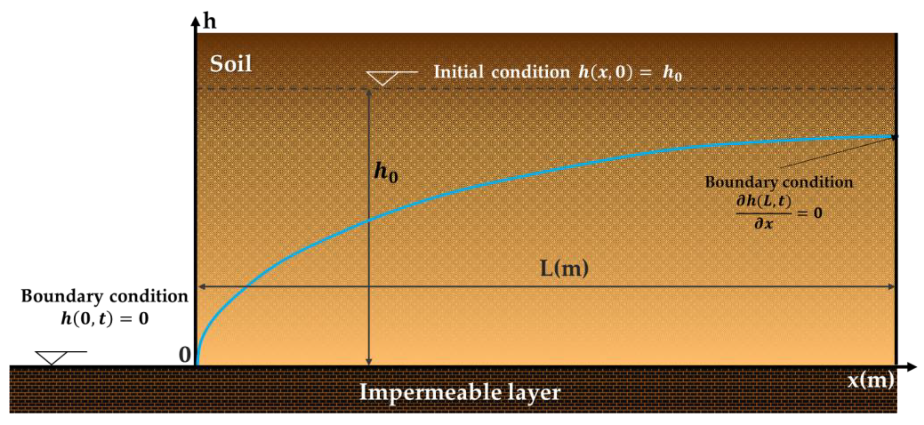
2.1. Crisp Model
Numerical Method
2.2. Fyzzy Framework and Definitions
- is increasing, is decreasing as functions of α, and
- , or
- is increasing, is decreasing as functions of α, and
- is (i)-gH-differentiable at x0 if:
- is (ii)-gH-differentiable at x0 if:
- is [(i)-p]-differentiable w.r.t. x at (x0, t0) if:
- is [(ii)-p]-differentiable w.r.t. x at (x0, t0) if:
- is [(i)-p]-differentiable w.r.t.x if:
- is [(ii)-p]-differentiable w.r.t.x if:
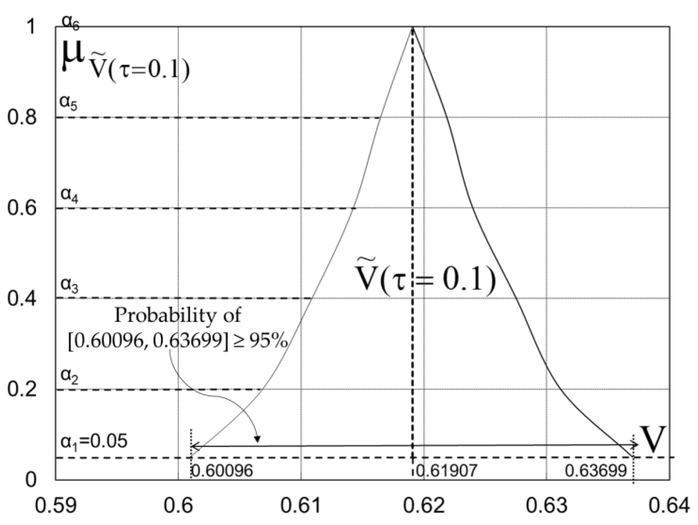
2.2.1. Possibility Theory
2.2.2. Fuzzy Model
| System (1,1): | System (1,2): |
| System (1,3): | System (1,4): |
| System (2,1): | System (2,2): |
| System (2,3): | System (2,4): |
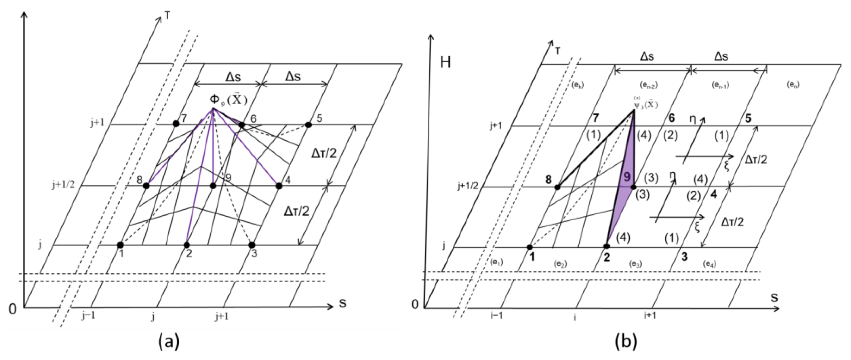
2.2.3. Fuzzy Finite Elements Solution
- From Equation (3), we have:
- 2.
- Another solution for Case a is putting it in the dimensional form:
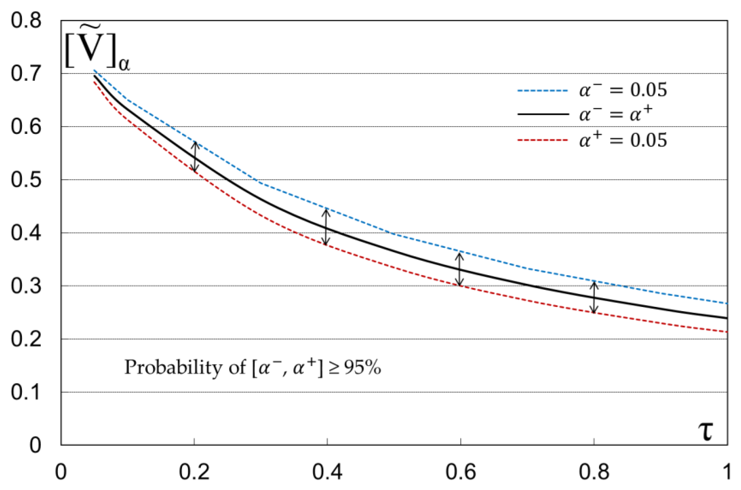
2.2.4. Outflow Volumes
2.3. A Proposed Method to Solve the Crisp and Fuzzy Models
| The Step-by-Step Solving Process | |
| Step 1: | The interval [s0, sN] is divided into N equal parts: |
| Step 2: | τ = τ + Δτ, |
| Step 3: | Initial valuesH(sr,0) sr, r = 1, 2, … N + 1 |
| Step 4: | Boundary values H(0,τ) = H0, |
| Step 5: | |
| Step 6: | Solve the tridiagonal system [34,70] |
| Step 7: | Put HNEW into HINITIAL |
| Step 8: | Compute outflow volume V(HNEW) |
| Step 9: | Print τ, V(τ), HΝΕW values |
| Step 10: | If go to 2 |
| end | |
3. Results—Application
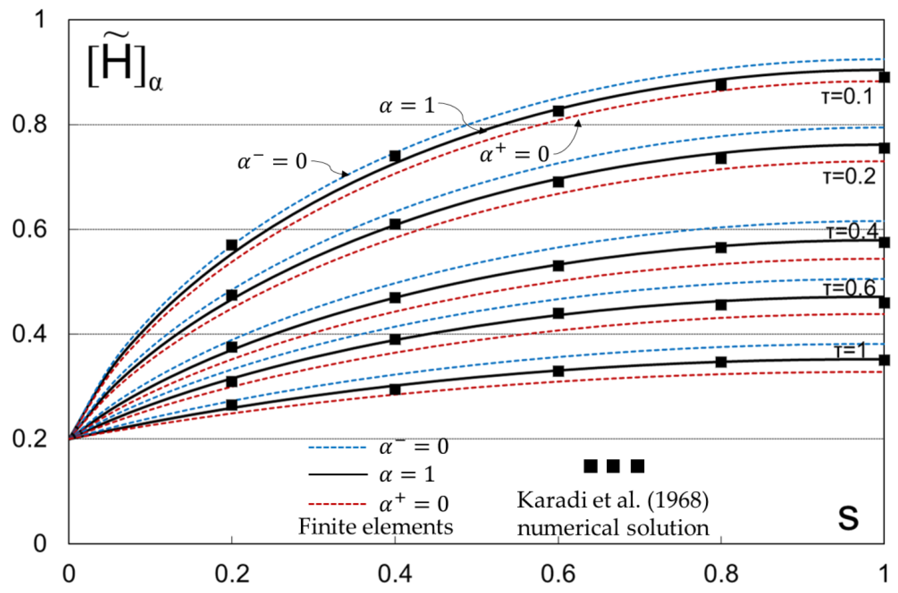
3.1. The Case by Karadi [68]
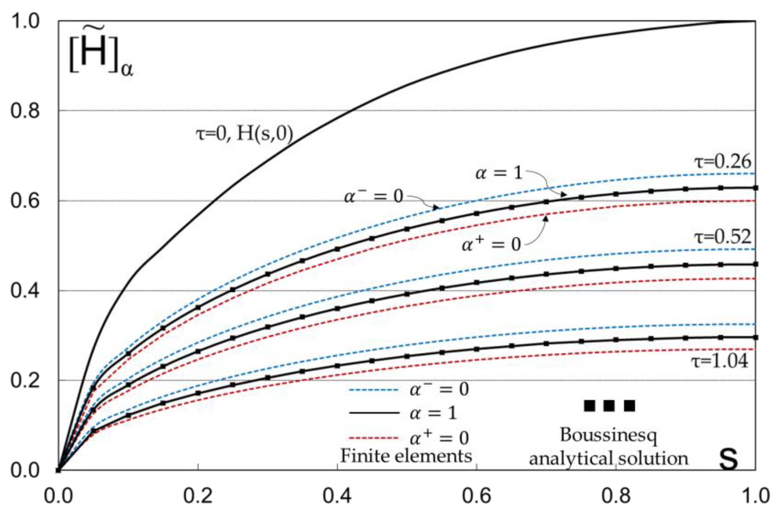
3.2. The Case for the Boussinesq Analytical Solution (1904)
- (a)
- Neglecting the effect of capillary rise above the water table;
- (b)
- Accepting the Dupuit-Forcheimer approximation, i.e., the hydraulic head is independent of depth, and therefore, the streamlines are assumed to be approximately parallel to the bed;
- (c)
- His solution is valid when t is large, that is, when the water table at x = L is below the aquifer depth h0. (See Figure 1).
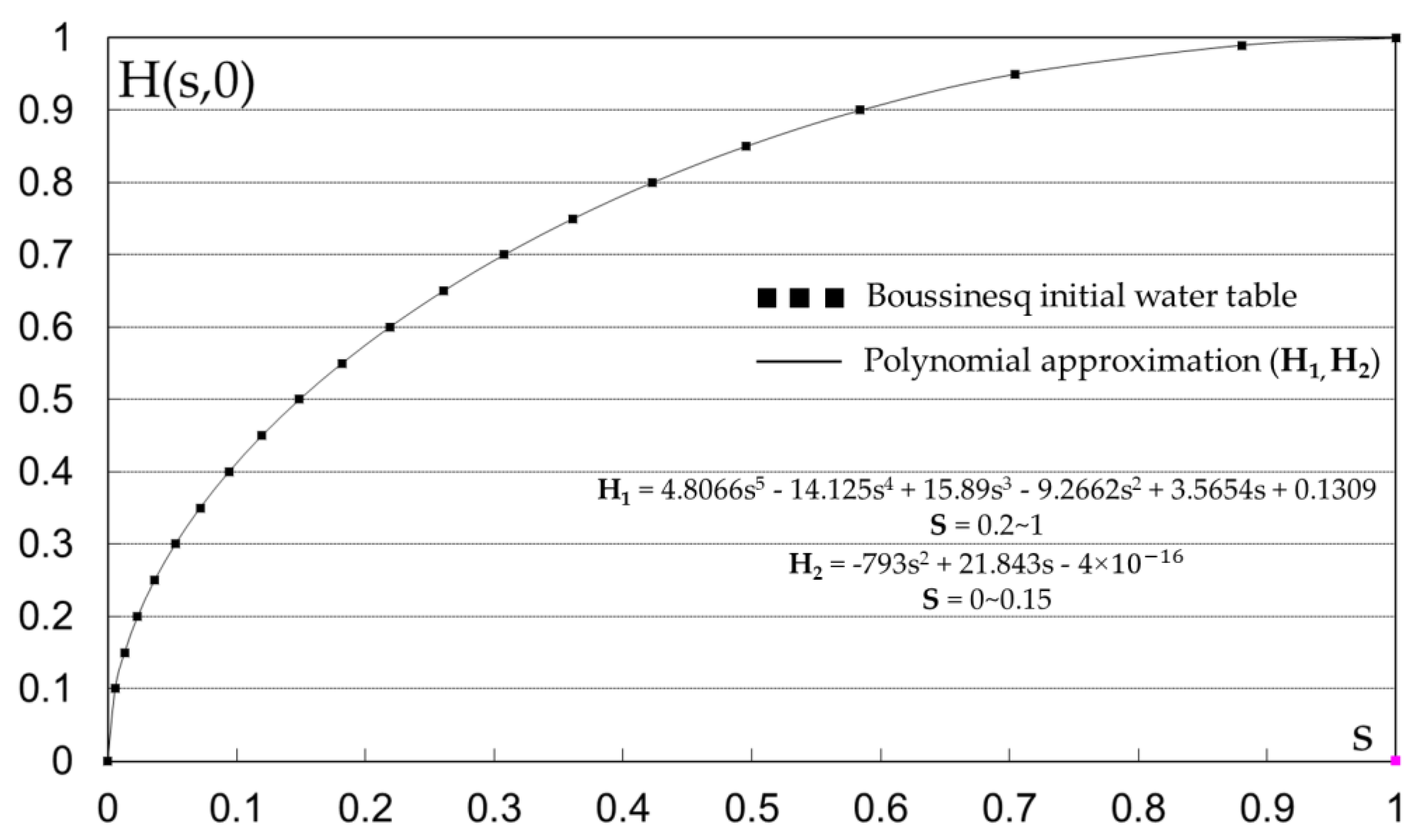
3.2.1. Initial Water Table
3.2.2. Water Table Equation
3.2.3. Outflow Volume
3.2.4. Discharge

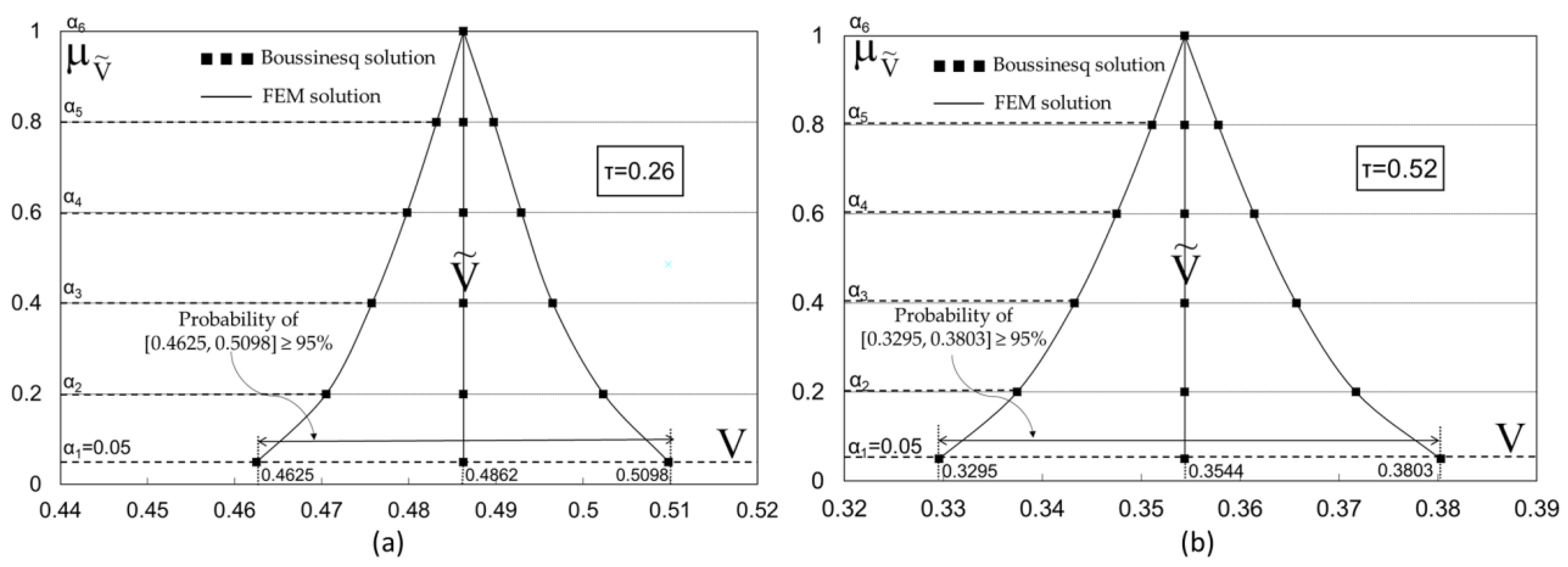
| α-Cut | |||
|---|---|---|---|
| Method | |||
| τ = 0.26 | |||
| FEM | 0.5098587 | 0.486479 | 0.46283113 |
| Boussinesq | 0.5104053 | 0.486995 | 0.46331698 |
| δ | 5.47 × 10⁻⁴ | 5.16× 10⁻⁴ | 4.86× 10⁻⁴ |
| Average = 5.16 × 10⁻⁴ | |||
| τ = 0.52 | |||
| FEM | 0.3802688 | 0.329547 | 0.354413 |
| Boussinesq | 0.3818421 | 0.331422 | 0.35621128 |
| δ | 1.57 × 10⁻³ | 1.88 × 10⁻³ | 1.80 × 10⁻³ |
| Average = 1.75 × 10⁻³ | |||
4. Discussion and Future Research
4.1. Significance of Incorporating Uncertainty in Groundwater Modeling
4.2. The Role of the Fuzzy Finite Element Method for Solving the Boussinesq Equation
4.3. Model Validation with Existing Solutions and Practical Applications
4.4. Limitations and Future Perspectives
5. Conclusions
Author Contributions
Funding
Data Availability Statement
Conflicts of Interest
References
- Boussinesq, J. Recherches Theoriques Sur l’ecoulement Des Nappes d’eau Infiltrees Dans Le Sol et Sur Le Debit Des Sources. J. Math. Pures Appl. 1904, 10, 5–78. [Google Scholar]
- Polubarinova-Kochina, P.Y. On a Non-Linear Differential Equation Occurring in Seepage Theory. DAN 1948, 36. [Google Scholar]
- Polubarinova-Kochina, P.Y. On Unsteady Motions of Groundwater during Seepage from Water Reservoirs. P.M.M. (Prinkladaya Mat. I Mekhanica) 1949, 13. [Google Scholar]
- Polubarinova-Kochina, P.Y. Theory of Groundwater Movement, 2015th ed.; Princeton University Press: Princeton, NJ, USA, 2015. [Google Scholar]
- Tolikas, P.K.; Sidiropoulos, E.G.; Tzimopoulos, C.D. A Simple Analytical Solution for the Boussinesq One-Dimensional Groundwater Flow Equation. Water Resour. Res. 1984, 20, 24–28. [Google Scholar] [CrossRef]
- Lockington, D.A. Response of Unconfined Aquifer to Sudden Change in Boundary Head. J. Irrig. Drain. Eng. 1997, 123, 24–27. [Google Scholar] [CrossRef]
- Moutsopoulos, K.N. The Analytical Solution of the Boussinesq Equation for Flow Induced by a Step Change of the Water Table Elevation Revisited. Transp. Porous Media 2010, 85, 919–940. [Google Scholar] [CrossRef]
- Basha, H.A. Traveling Wave Solution of the Boussinesq Equation for Groundwater Flow in Horizontal Aquifers. Water Resour. Res. 2013, 49, 1668–1679. [Google Scholar] [CrossRef]
- Chor, T.; Dias, N.L.; de Zárate, A.R. An Exact Series and Improved Numerical and Approximate Solutions for the Boussinesq Equation. Water Resour. Res. 2013, 49, 7380–7387. [Google Scholar] [CrossRef]
- Hayek, M. Accurate Approximate Semi-Analytical Solutions to the Boussinesq Groundwater Flow Equation for Recharging and Discharging of Horizontal Unconfined Aquifers. J. Hydrol. 2019, 570, 411–422. [Google Scholar] [CrossRef]
- Khan, H.; Farooq, U.; Shah, R.; Baleanu, D.; Kumam, P.; Arif, M. Analytical Solutions of (2+Time Fractional Order) Dimensional Physical Models, Using Modified Decomposition Method. Appl. Sci. 2019, 10, 122. [Google Scholar] [CrossRef]
- Shah, R.; Khan, H.; Kumam, P.; Arif, M. An Analytical Technique to Solve the System of Nonlinear Fractional Partial Differential Equations. Mathematics 2019, 7, 505. [Google Scholar] [CrossRef]
- Rashid, S.; Khalid, A.; Sultana, S.; Hammouch, Z.; Shah, R.; Alsharif, A.M. A Novel Analytical View of Time-Fractional Korteweg-De Vries Equations via a New Integral Transform. Symmetry 2021, 13, 1254. [Google Scholar] [CrossRef]
- Iqbal, N.; Akgül, A.; Shah, R.; Bariq, A.; Mossa Al-Sawalha, M.; Ali, A. On Solutions of Fractional-Order Gas Dynamics Equation by Effective Techniques. J. Funct. Spaces 2022, 2022, 3341754. [Google Scholar] [CrossRef]
- Tzimopoulos, C.; Papadopoulos, K.; Evangelides, C.; Spyrides, A. Recharging and Discharging of Unconfined Aquifers. Case of Nonlinear Boussinesq Equation. In Proceedings of the Eighth International Conference on Environmental Management,Engineering, Planning and Economics (CEMEPE 2021) and SECOTOX Conference, CEMEPE 2021, Thessaloniki, Greece, 22 June 2021; pp. 74–80. [Google Scholar]
- Wiedeburg, O. Ueber Die Hydrodiffusion. Ann. Phys. 1890, 277, 675–711. [Google Scholar] [CrossRef]
- Chen, Z.-X.; Bodvarsson, G.S.; Witherspoon, P.A.; Yortsos, Y.C. An Integral Equation Formulation for the Unconfined Flow of Groundwater with Variable Inlet Conditions. Transp. Porous Media 1995, 18, 15–36. [Google Scholar] [CrossRef]
- Parlange, J.-Y.; Hogarth, W.L.; Govindaraju, R.S.; Parlange, M.B.; Lockington, D. On an Exact Analytical Solution of the Boussinesq Equation. Transp. Porous Media 2000, 39, 339–345. [Google Scholar] [CrossRef]
- Telyakovskiy, A.S.; Braga, G.A.; Furtado, F. Approximate Similarity Solutions to the Boussinesq Equation. Adv. Water Resour. 2002, 25, 191–194. [Google Scholar] [CrossRef]
- Pistiner, A. Similarity Solution to Unconfined Flow in an Aquifer. Transp. Porous Media 2008, 71, 265–272. [Google Scholar] [CrossRef]
- Olsen, J.S.; Telyakovskiy, A.S. Polynomial Approximate Solutions of a Generalized Boussinesq Equation. Water Resour. Res. 2013, 49, 3049–3053. [Google Scholar] [CrossRef]
- Bartlett, M.S.; Porporato, A. A Class of Exact Solutions of the Boussinesq Equation for Horizontal and Sloping Aquifers. Water Resour. Res. 2018, 54, 767–778. [Google Scholar] [CrossRef]
- Tzimopoulos, C.; Papadopoulos, K.; Evangelides, C.; Papadopoulos, B. Fuzzy Solution to the Unconfined Aquifer Problem. Water 2018, 1, 54. [Google Scholar] [CrossRef]
- Remson, I.; Hornberger, G.; Moltz, F. Numerical Methods in Subsurface Hydrology; Wiley-Interscience: Toronto, ON, Canada, 1971. [Google Scholar]
- Tzimopoulos, C.; Terzidis, G. Écoulement Non Permanent Dans Un Sol Drainé Par Des Fossés Parallèles. J. Hydrol. 1975, 27, 73–93. [Google Scholar] [CrossRef]
- Chávez, C.; Fuentes, C.; Zavala, M.; Brambila, F. Numerical Solution of the Boussinesq Equation. Application to the Agricultural Drainage. Afr. J. Agric. Res. 2011, 18, 4210–4222. [Google Scholar]
- Bansal, R.K. Groundwater Fluctuations in Sloping Aquifers Induced by Time-Varying Replenishment and Seepage from a Uniformly Rising Stream. Transp. Porous Media 2012, 94, 817–836. [Google Scholar] [CrossRef]
- Bansal, K.R. Approximate Analytical Solution of Boussinesq Equation in Homogeneous Medium with Leaky Base. Appl. Appl. Math. Int. J. (AAM) 2016, 11, 184–191. [Google Scholar]
- Borana, R.N.; Pradhan, V.H.; Mehta, N. Numerical Solution of Boussinesq Equation Arising in One-Dimensional Infiltration Phenomenon by Using Finite Difference Method. Int. J. Res. Eng. Technol. 2013, 2, 202–209. [Google Scholar]
- Bansal, R.K. Unsteady Seepage Flow over Sloping Beds in Response to Multiple Localized Recharge. Appl. Water Sci. 2017, 7, 777–786. [Google Scholar] [CrossRef][Green Version]
- Nguyen, T. Numerical and Analytical Analysis of Flow in Stratified Heterogeneous Porous Media. Master’s Thesis, University of Stavanger, Stavanger, Norway, 2018. [Google Scholar]
- Samarinas, N.; Tzimopoulos, C.; Evangelides, C. Fuzzy Numerical Solution to Horizontal Infiltration. Int. J. Circuits Syst. Signal Process. 2018, 12, 326–332. [Google Scholar]
- Samarinas, N.; Tzimopoulos, C.; Evangelides, C. Fuzzy Numerical Solution to the Unconfined Aquifer Problem under the Boussinesq Equation. Water Supply 2021, 21, 3210–3224. [Google Scholar] [CrossRef]
- Samarinas, N.; Tzimopoulos, C.; Evangelides, C. An Efficient Method to Solve the Fuzzy Crank–Nicolson Scheme with Application to the Groundwater Flow Problem. J. Hydroinform. 2022, 24, 590–609. [Google Scholar] [CrossRef]
- Courant, R. Variational Methods for the Solution of Problems of Equilibrium and Vibrations. Bull. Am. Math. Soc. 1943, 49, 1–23. [Google Scholar] [CrossRef]
- Argyris, J.H. Energy Theorems and Structural Analysis. Aircr. Eng. Aerosp. Technol. 1954, 26, 383–394. [Google Scholar] [CrossRef]
- Turner, M.J.; Clough, R.W.; Martin, H.C.; Topp, L.J. Stiffness and Deflection Analysis of Complex Structures. J. Aeronaut. Sci. 1956, 23, 805–823. [Google Scholar] [CrossRef]
- Oden, J.T. Historical Comments on Finite Elements. In A History of Scientific Computing; ACM: New York, NY, USA, 1990; pp. 152–166. [Google Scholar]
- Tzimopoulos, C. Solution de l’équation de Boussinesq Par Une Méthode Des Éléments Finis. J. Hydrol. 1976, 30, 1–18. [Google Scholar] [CrossRef]
- Galerkin, B.G. Rods and Plates: Series in Some Questions of Elastic Equilibrium of Rods and Plates; National Technical Information Service: Springfield, VA, USA, 1968. [Google Scholar]
- Frangakis, C.N.; Tzimopoulos, C. Unsteady Groundwater Flow on Sloping Bedrock. Water Resour. Res. 1979, 15, 176–180. [Google Scholar] [CrossRef]
- Tzimopoulos, C.; Tolikas, P. Technical and theoretical aspects in artificial ground water recharge. ICID Bull. Int. Comm. Irrig. Drain. 1980, 29, 40–44. [Google Scholar]
- Tber, M.H.; El Alaoui Talibi, M. A Finite Element Method for Hydraulic Conductivity Identification in a Seawater Intrusion Problem. Comput. Geosci. 2007, 33, 860–874. [Google Scholar] [CrossRef]
- Mohammadnejad, T.; Khoei, A.R. An Extended Finite Element Method for Hydraulic Fracture Propagation in Deformable Porous Media with the Cohesive Crack Model. Finite Elem. Anal. Des. 2013, 73, 77–95. [Google Scholar] [CrossRef]
- Yang, D.; Zhou, Y.; Xia, X.; Gu, S.; Xiong, Q.; Chen, W. Extended Finite Element Modeling Nonlinear Hydro-Mechanical Process in Saturated Porous Media Containing Crossing Fractures. Comput. Geotech. 2019, 111, 209–221. [Google Scholar] [CrossRef]
- Aslan, T.A.; Temel, B. Finite Element Analysis of the Seepage Problem in the Dam Body and Foundation Based on the Galerkin’s Approach. Eur. Mech. Sci. 2022, 6, 143–151. [Google Scholar] [CrossRef]
- Ritz, W. Über Eine Neue Methode Zur Lösung Gewisser Variationsprobleme Der Mathematischen Physik. J. Die Reine Angew. Math. 1909, 1909, 1–61. [Google Scholar] [CrossRef]
- Puri, M.L.; Ralescu, D.A. Differentials of Fuzzy Functions. J. Math. Anal. Appl. 1983, 91, 552–558. [Google Scholar] [CrossRef]
- Hukuhara, M. Integration Des Applications Measurables Dont La Valeur Est Un Compact Convexe. Funkc. Ekvacioj 1967, 10, 205–233. [Google Scholar]
- Kaleva, O. Fuzzy Differential Equations. Fuzzy Sets Syst. 1987, 24, 301–307. [Google Scholar] [CrossRef]
- Seikkala, S. On the Fuzzy Initial Value Problem. Fuzzy Sets Syst. 1987, 24, 319–330. [Google Scholar] [CrossRef]
- Vorobiev, D.; Seikkala, S. Towards the Theory of Fuzzy Differential Equations. Fuzzy Sets Syst. 2002, 125, 231–237. [Google Scholar] [CrossRef]
- O’Regan, D.; Lakshmikantham, V.; Nieto, J.J. Initial and Boundary Value Problem for Fuzzy Differential Equations. Nonlinear Anal. 2003, 54, 405–415. [Google Scholar] [CrossRef]
- Nieto, J.J.; Rodríguez-López, R. Bounded Solutions for Fuzzy Differential and Integral Equations. Chaos Solitons Fractals 2006, 27, 1376–1386. [Google Scholar] [CrossRef]
- Diamond, P. Brief Note on the Variation of Constants Formula for Fuzzy Differential Equations. Fuzzy Sets Syst. 2002, 129, 65–71. [Google Scholar] [CrossRef]
- Bede, B.; Gal, S.G. Generalizations of the Differentiability of Fuzzy-Number-Valued Functions with Applications to Fuzzy Differential Equations. Fuzzy Sets Syst. 2005, 151, 581–599. [Google Scholar] [CrossRef]
- Stefanini, L. A Generalization of Hukuhara Difference and Division for Interval and Fuzzy Arithmetic. Fuzzy Sets Syst. 2010, 161, 1564–1584. [Google Scholar] [CrossRef]
- Allahviranloo, T.; Gouyandeh, Z.; Armand, A.; Hasanoglu, A. On Fuzzy Solutions for Heat Equation Based on Generalized Hukuhara Differentiability. Fuzzy Sets Syst. 2015, 265, 1–23. [Google Scholar] [CrossRef]
- Rodríguez Pérez, Á.M.; Rodríguez, C.A.; Olmo Rodríguez, L.; Caparros Mancera, J.J. Revitalizing the Canal de Castilla: A Community Approach to Sustainable Hydropower Assessed through Fuzzy Logic. Appl. Sci. 2024, 14, 1828. [Google Scholar] [CrossRef]
- Rodríguez-Pérez, Á.M.; Rodríguez, C.A.; Márquez-Rodríguez, A.; Mancera, J.J.C. Viability Analysis of Tidal Turbine Installation Using Fuzzy Logic: Case Study and Design Considerations. Axioms 2023, 12, 778. [Google Scholar] [CrossRef]
- Tzimopoulos, C.; Evangelides, C.; Vrekos, C.; Samarinas, N. Fuzzy Linear Regression of Rainfall-Altitude Relationship. Proceedings 2018, 2, 636. [Google Scholar] [CrossRef]
- Samarinas, N.; Evangelides, C. Discharge Estimation for Trapezoidal Open Channels Applying Fuzzy Transformation Method to a Flow Equation. Water Supply 2021, 21, 2893–2903. [Google Scholar] [CrossRef]
- Tzimopoulos, C.; Papadopoulos, K.; Papadopoulos, B.; Samarinas, N.; Evangelides, C. Fuzzy Solution of Nonlinear Boussinesq Equation. J. Hydroinform. 2022, 24, 1127–1147. [Google Scholar] [CrossRef]
- Cherki, A.; Plessis, G.; Lallemand, B.; Tison, T.; Level, P. Fuzzy Behavior of Mechanical Systems with Uncertain Boundary Conditions. Comput. Methods Appl. Mech. Eng. 2000, 189, 863–873. [Google Scholar] [CrossRef]
- Behera, D.; Chakraverty, S. Fuzzy Finite Element Based Solution of Uncertain Static Problems of Structural Mechanics. Int. J. Comput. Appl. 2013, 59, 69–75. [Google Scholar] [CrossRef]
- Ranjit, D.K.; Roy, T.K. Fuzzy Finite Element Method Applied to Euler-Bernoulli Beam Problem. Int. J. Math. Trends Technol. 2018, 53, 304–320. [Google Scholar] [CrossRef]
- Rodríguez, C.A.; Rodríguez-Pérez, Á.M.; López, R.; Hernández-Torres, J.A.; Caparrós-Mancera, J.J. A Finite Element Method Integrated with Terzaghi’s Principle to Estimate Settlement of a Building Due to Tunnel Construction. Buildings 2023, 13, 1343. [Google Scholar] [CrossRef]
- Karadi, G.; Krizek, R.J.; Elnaggar, H. Unsteady Seepage Flow between Fully-Penetrating Trenches. J. Hydrol. 1968, 6, 417–430. [Google Scholar] [CrossRef]
- Oden, J.T. Finite Elements of Nonlinear Continua; Dover Publications: Mineola, NY, USA, 1972. [Google Scholar]
- Thomas, L.H. Elliptic Problems in Linear Differential Equations over a Network; Watson Sci Lab Report Columbia University: New York, NY, USA, 1949. [Google Scholar]
- Negoiţă, C.V.; Ralescu, D.A. Applications of Fuzzy Sets to Systems Analysis; Birkhäuser: Basel, Switzerland, 1975. [Google Scholar]
- Goetshel, R.; Voxman, W. Elementary Fuzzy Calculus. Fuzzy Sets Syst. 1986, 18, 31–43. [Google Scholar] [CrossRef]
- Bede, B.; Stefanini, L. Generalized Differentiability of Fuzzy-Valued Functions. Fuzzy Sets Syst. 2013, 230, 119–141. [Google Scholar] [CrossRef]
- Khastan, A.; Nieto, J.J. A Boundary Value Problem for Second Order Fuzzy Differential Equations. Nonlinear Anal. Theory Methods Appl. 2010, 72, 3583–3593. [Google Scholar] [CrossRef]
- Dubois, D.; Foulloy, L.; Mauris, G.; Prade, H. Probability-Possibility Transformations, Triangular Fuzzy Sets, and Probabilistic Inequalities. Reliab. Comput. 2004, 10, 273–297. [Google Scholar] [CrossRef]
- Mylonas, N. Applications in Fuzzy Statistic and Approximate Reasoning. Ph.D. Thesis, Dimoktritos University of Thrace, Xanthi, Greece, 2022. [Google Scholar]
- Tzimopoulos, C.; Samarinas, N.; Papadopoulos, K.; Evangelides, C. Fuzzy Unsteady-State Drainage Solution for Land Reclamation. Hydrology 2023, 10, 34. [Google Scholar] [CrossRef]
- Richard, G.; Sillon, J.F.; Marloie, O. Comparison of Inverse and Direct Evaporation Methods for Estimating Soil Hydraulic Properties under Different Tillage Practices. Soil. Sci. Soc. Am. J. 2001, 65, 215–224. [Google Scholar] [CrossRef]
- Richard, G.; Cousin, I.; Sillon, J.F.; Bruand, A.; Guérif, J. Effect of Compaction on the Porosity of a Silty Soil: Influence on Unsaturated Hydraulic Properties. Eur. J. Soil. Sci. 2001, 52, 49–58. [Google Scholar] [CrossRef]
- Anderskouv, K.; Surlyk, F. The Influence of Depositional Processes on the Porosity of Chalk. J. Geol. Soc. Lond. 2012, 169, 311–325. [Google Scholar] [CrossRef]
- Carbillet, L.; Heap, M.J.; Baud, P.; Wadsworth, F.B.; Reuschlé, T. The Influence of Grain Size Distribution on Mechanical Compaction and Compaction Localization in Porous Rocks. J. Geophys. Res. Solid. Earth 2022, 127, e2022JB025216. [Google Scholar] [CrossRef]
- Van Lopik, J.H.; Snoeijers, R.; van Dooren, T.C.G.W.; Raoof, A.; Schotting, R.J. The Effect of Grain Size Distribution on Nonlinear Flow Behavior in Sandy Porous Media. Transp. Porous Media 2017, 120, 37–66. [Google Scholar] [CrossRef]
- Sihag, P. Prediction of Unsaturated Hydraulic Conductivity Using Fuzzy Logic and Artificial Neural Network. Model. Earth Syst. Environ. 2018, 4, 189–198. [Google Scholar] [CrossRef]
- More, S.B.; Deka, P.C. Estimation of Saturated Hydraulic Conductivity Using Fuzzy Neural Network in a Semi-Arid Basin Scale for Murum Soils of India. ISH J. Hydraul. Eng. 2018, 24, 140–146. [Google Scholar] [CrossRef]
- Ross, J.; Ozbek, M.; Pinder, G.F. Hydraulic Conductivity Estimation via Fuzzy Analysis of Grain Size Data. Math. Geol. 2007, 39, 765–780. [Google Scholar] [CrossRef]


| s | H(s,0) | s | H(s,0) | s | H(s,0) | s | H(s,0) |
|---|---|---|---|---|---|---|---|
| s0 | 0.000 | s6 | 0.689 | s12 | 0.909 | s18 | 0.990 |
| s1 | 0.250 | s7 | 0.740 | s13 | 0.930 | s19 | 0.997 |
| s2 | 0.417 | s8 | 0.784 | s14 | 0.947 | s20 | 1.000 |
| s3 | 0.497 | s9 | 0.823 | s15 | 0.961 | ||
| s4 | 0.568 | s10 | 0.857 | s16 | 0.972 | ||
| s5 | 0.633 | s11 | 0.885 | s17 | 0.982 |
| FEM | Boussinesq | FEM vs. Boussinesq | |||||||
|---|---|---|---|---|---|---|---|---|---|
| s | 0.22751 | 0.296197 | 0.26 | 0.22751 | 0.296197 | 0.26 | |||
| 0.00 | 0.00000 | 0.00000 | 0.00000 | 0.00000 | 0.00000 | 0.00000 | 0.00000 | 0.00000 | 0.00000 |
| 0.05 | 0.19392 | 0.17600 | 0.18499 | 0.19100 | 0.17338 | 0.18224 | 0.01505558 | 0.002919578 | 0.002618113 |
| 0.10 | 0.27306 | 0.24783 | 0.26049 | 0.27154 | 0.24649 | 0.25909 | 0.00557023 | 0.001521008 | 0.001338698 |
| 0.15 | 0.33244 | 0.30172 | 0.31713 | 0.33440 | 0.30356 | 0.31907 | 0.00590884 | 0.001964334 | 0.001837729 |
| 0.20 | 0.38111 | 0.34588 | 0.36356 | 0.38438 | 0.34892 | 0.36675 | 0.00857316 | 0.003267318 | 0.003041032 |
| 0.25 | 0.42257 | 0.38350 | 0.40310 | 0.42519 | 0.38597 | 0.40569 | 0.00620473 | 0.002621934 | 0.002470768 |
| 0.30 | 0.45860 | 0.41619 | 0.43747 | 0.45965 | 0.41725 | 0.43857 | 0.00230021 | 0.001054877 | 0.001064731 |
| 0.35 | 0.49028 | 0.44492 | 0.46768 | 0.48977 | 0.44459 | 0.46730 | 0.00105017 | 0.000514879 | 0.000332497 |
| 0.40 | 0.51827 | 0.47031 | 0.49437 | 0.51683 | 0.46916 | 0.49313 | 0.00277172 | 0.001436498 | 0.001150997 |
| 0.45 | 0.54306 | 0.49278 | 0.51801 | 0.54160 | 0.49164 | 0.51676 | 0.00268424 | 0.001457705 | 0.001136963 |
| 0.50 | 0.56499 | 0.51266 | 0.53891 | 0.56436 | 0.51231 | 0.53848 | 0.00110658 | 0.000625205 | 0.000354154 |
| 0.55 | 0.58430 | 0.53015 | 0.55732 | 0.58508 | 0.53111 | 0.55825 | 0.00134331 | 0.000784895 | 0.000964653 |
| 0.60 | 0.60119 | 0.54545 | 0.57341 | 0.60352 | 0.54785 | 0.57584 | 0.0038701 | 0.002326665 | 0.002396213 |
| 0.65 | 0.61580 | 0.55867 | 0.58733 | 0.61932 | 0.56220 | 0.59092 | 0.00572253 | 0.003523935 | 0.003525366 |
| 0.70 | 0.62825 | 0.56994 | 0.59919 | 0.63220 | 0.57388 | 0.60321 | 0.00628709 | 0.003949867 | 0.003943577 |
| 0.75 | 0.63863 | 0.57931 | 0.60907 | 0.64199 | 0.58277 | 0.61254 | 0.00525585 | 0.003356541 | 0.003457496 |
| 0.80 | 0.64701 | 0.58687 | 0.61704 | 0.64879 | 0.58895 | 0.61904 | 0.00275812 | 0.001784533 | 0.002077495 |
| 0.85 | 0.65344 | 0.59265 | 0.62314 | 0.65312 | 0.59288 | 0.62317 | 0.0004859 | 0.000317509 | 0.000226227 |
| 0.90 | 0.65795 | 0.59669 | 0.62741 | 0.65598 | 0.59547 | 0.62589 | 0.00299914 | 0.001973282 | 0.00122283 |
| 0.95 | 0.66057 | 0.59901 | 0.62988 | 0.65899 | 0.59820 | 0.62877 | 0.00239074 | 0.001579253 | 0.000806825 |
| 1.00 | 0.66131 | 0.59960 | 0.63056 | 0.66342 | 0.60222 | 0.63299 | 0.00318628 | 0.002107117 | 0.002621241 |
| 1.86 × 10⁻³ | 1.74 × 10⁻³ | 1.80 × 10⁻³ | |||||||
| Average = 1.80114 × 10⁻³ | |||||||||
| FEM | Boussinesq | FEM vs. Boussinesq | |||||||
|---|---|---|---|---|---|---|---|---|---|
| s | 0.22751 | 0.296197 | 0.26 | 0.22751 | 0.296197 | 0.26 | |||
| 0.00 | 0.00000 | 0.00000 | 0.00000 | 0.00000 | 0.00000 | 0.00000 | 0.000000 | 0.000000 | 0.000000 |
| 0.05 | 0.14481 | 0.12549 | 0.13493 | 0.14291 | 0.12404 | 0.13331 | 0.001905 | 0.001450 | 0.001616 |
| 0.10 | 0.20390 | 0.17670 | 0.18998 | 0.20316 | 0.17634 | 0.18953 | 0.000736 | 0.000356 | 0.000453 |
| 0.15 | 0.24823 | 0.21511 | 0.23128 | 0.25020 | 0.21717 | 0.23341 | 0.001969 | 0.002060 | 0.002126 |
| 0.20 | 0.28456 | 0.24658 | 0.26512 | 0.28759 | 0.24962 | 0.26829 | 0.003028 | 0.003044 | 0.003166 |
| 0.25 | 0.31549 | 0.27337 | 0.29394 | 0.31813 | 0.27613 | 0.29677 | 0.002636 | 0.002760 | 0.002833 |
| 0.30 | 0.34236 | 0.29665 | 0.31897 | 0.34391 | 0.29851 | 0.32083 | 0.001551 | 0.001861 | 0.001858 |
| 0.35 | 0.36597 | 0.31710 | 0.34096 | 0.36644 | 0.31807 | 0.34184 | 0.000469 | 0.000965 | 0.000884 |
| 0.40 | 0.38683 | 0.33515 | 0.36038 | 0.38669 | 0.33564 | 0.36074 | 0.000139 | 0.000494 | 0.000357 |
| 0.45 | 0.40529 | 0.35113 | 0.37757 | 0.40522 | 0.35173 | 0.37802 | 0.000067 | 0.000600 | 0.000455 |
| 0.50 | 0.42160 | 0.36524 | 0.39276 | 0.42225 | 0.36651 | 0.39391 | 0.000654 | 0.001272 | 0.001153 |
| 0.55 | 0.43595 | 0.37765 | 0.40611 | 0.43776 | 0.37997 | 0.40837 | 0.001807 | 0.002318 | 0.002265 |
| 0.60 | 0.44848 | 0.38849 | 0.41778 | 0.45155 | 0.39194 | 0.42124 | 0.003067 | 0.003448 | 0.003460 |
| 0.65 | 0.45931 | 0.39785 | 0.42785 | 0.46337 | 0.40220 | 0.43227 | 0.004064 | 0.004354 | 0.004423 |
| 0.70 | 0.46852 | 0.40579 | 0.43641 | 0.47301 | 0.41057 | 0.44126 | 0.004488 | 0.004776 | 0.004850 |
| 0.75 | 0.47617 | 0.41239 | 0.44353 | 0.48033 | 0.41692 | 0.44809 | 0.004160 | 0.004532 | 0.004561 |
| 0.80 | 0.48232 | 0.41768 | 0.44924 | 0.48542 | 0.42134 | 0.45284 | 0.003104 | 0.003663 | 0.003603 |
| 0.85 | 0.48701 | 0.42170 | 0.45358 | 0.48866 | 0.42415 | 0.45586 | 0.001652 | 0.002454 | 0.002283 |
| 0.90 | 0.49025 | 0.42447 | 0.45658 | 0.49080 | 0.42601 | 0.45786 | 0.000547 | 0.001537 | 0.001275 |
| 0.95 | 0.49208 | 0.42601 | 0.45826 | 0.49305 | 0.42796 | 0.45996 | 0.000972 | 0.001955 | 0.001699 |
| 1.00 | 0.49249 | 0.42632 | 0.45862 | 0.49636 | 0.43084 | 0.46305 | 0.003874 | 0.004519 | 0.004429 |
| 1.94702 × 10⁻³ | 2.30559 × 10⁻³ | 2.27369 × 10⁻³ | |||||||
| Average = 2.17543 × 10⁻³ | |||||||||
| α-Cut | |||
|---|---|---|---|
| Method | α− | α− | α− = α+ |
| τ = 0.26 | |||
| FEM | 0.5098587 | 0.486479 | 0.46283113 |
| Boussinesq | 0.5104053 | 0.486995 | 0.46331698 |
| δ | 5.47 × 10⁻⁴ | 5.16 × 10⁻⁴ | 4.86 × 10⁻⁴ |
| Average = 5.16 × 10⁻⁴ | |||
| τ = 0.52 | |||
| FEM | 0.3802688 | 0.329547 | 0.354413 |
| Boussinesq | 0.3818421 | 0.331422 | 0.35621128 |
| δ | 1.57 × 10⁻³ | 1.88 × 10⁻³ | 1.80 × 10⁻³ |
| Average = 1.75 × 10⁻³ | |||
Disclaimer/Publisher’s Note: The statements, opinions and data contained in all publications are solely those of the individual author(s) and contributor(s) and not of MDPI and/or the editor(s). MDPI and/or the editor(s) disclaim responsibility for any injury to people or property resulting from any ideas, methods, instructions or products referred to in the content. |
© 2024 by the authors. Licensee MDPI, Basel, Switzerland. This article is an open access article distributed under the terms and conditions of the Creative Commons Attribution (CC BY) license (https://creativecommons.org/licenses/by/4.0/).
Share and Cite
Tzimopoulos, C.; Papadopoulos, K.; Samarinas, N.; Papadopoulos, B.; Evangelides, C. Fuzzy Finite Elements Solution Describing Recession Flow in Unconfined Aquifers. Hydrology 2024, 11, 47. https://doi.org/10.3390/hydrology11040047
Tzimopoulos C, Papadopoulos K, Samarinas N, Papadopoulos B, Evangelides C. Fuzzy Finite Elements Solution Describing Recession Flow in Unconfined Aquifers. Hydrology. 2024; 11(4):47. https://doi.org/10.3390/hydrology11040047
Chicago/Turabian StyleTzimopoulos, Christos, Kyriakos Papadopoulos, Nikiforos Samarinas, Basil Papadopoulos, and Christos Evangelides. 2024. "Fuzzy Finite Elements Solution Describing Recession Flow in Unconfined Aquifers" Hydrology 11, no. 4: 47. https://doi.org/10.3390/hydrology11040047
APA StyleTzimopoulos, C., Papadopoulos, K., Samarinas, N., Papadopoulos, B., & Evangelides, C. (2024). Fuzzy Finite Elements Solution Describing Recession Flow in Unconfined Aquifers. Hydrology, 11(4), 47. https://doi.org/10.3390/hydrology11040047