
The Importance of Solving Subglaciar Hydrology in Modeling Glacier Retreat: A Case Study of Hansbreen, Svalbard


Abstract
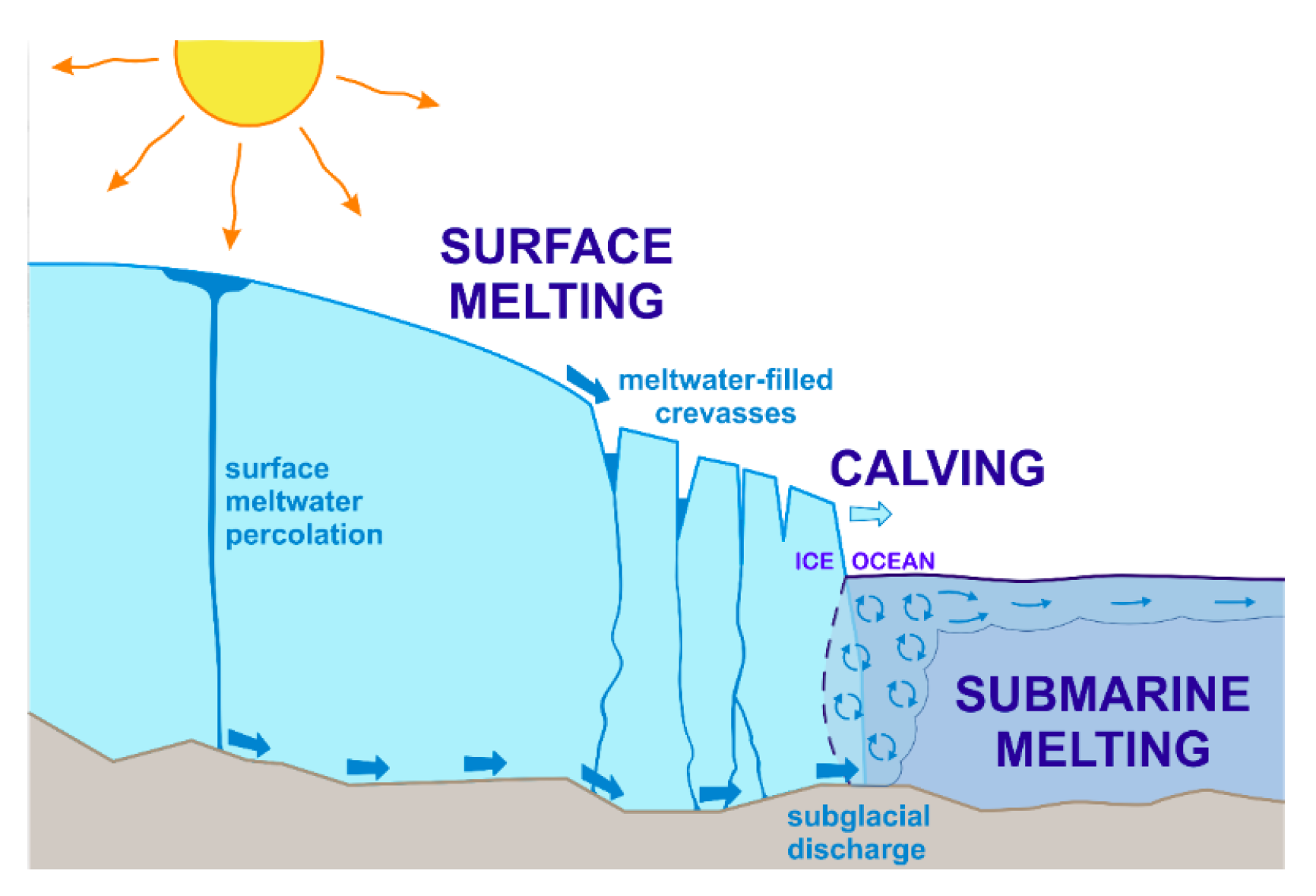
1. Introduction
2. Materials and Methods
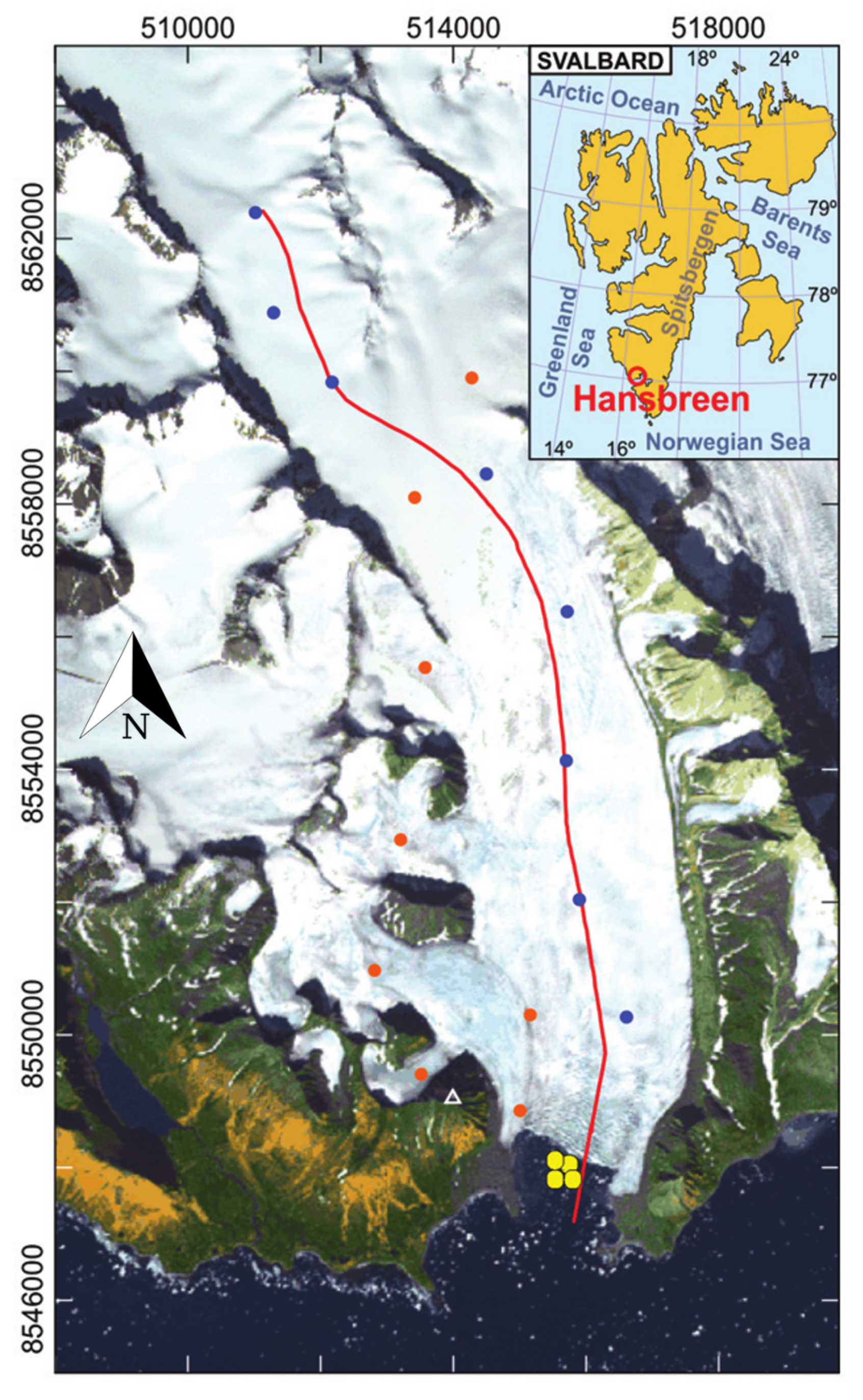
2.1. The Glacier–Fjord System of Study: Hansbreen-Hansbukta
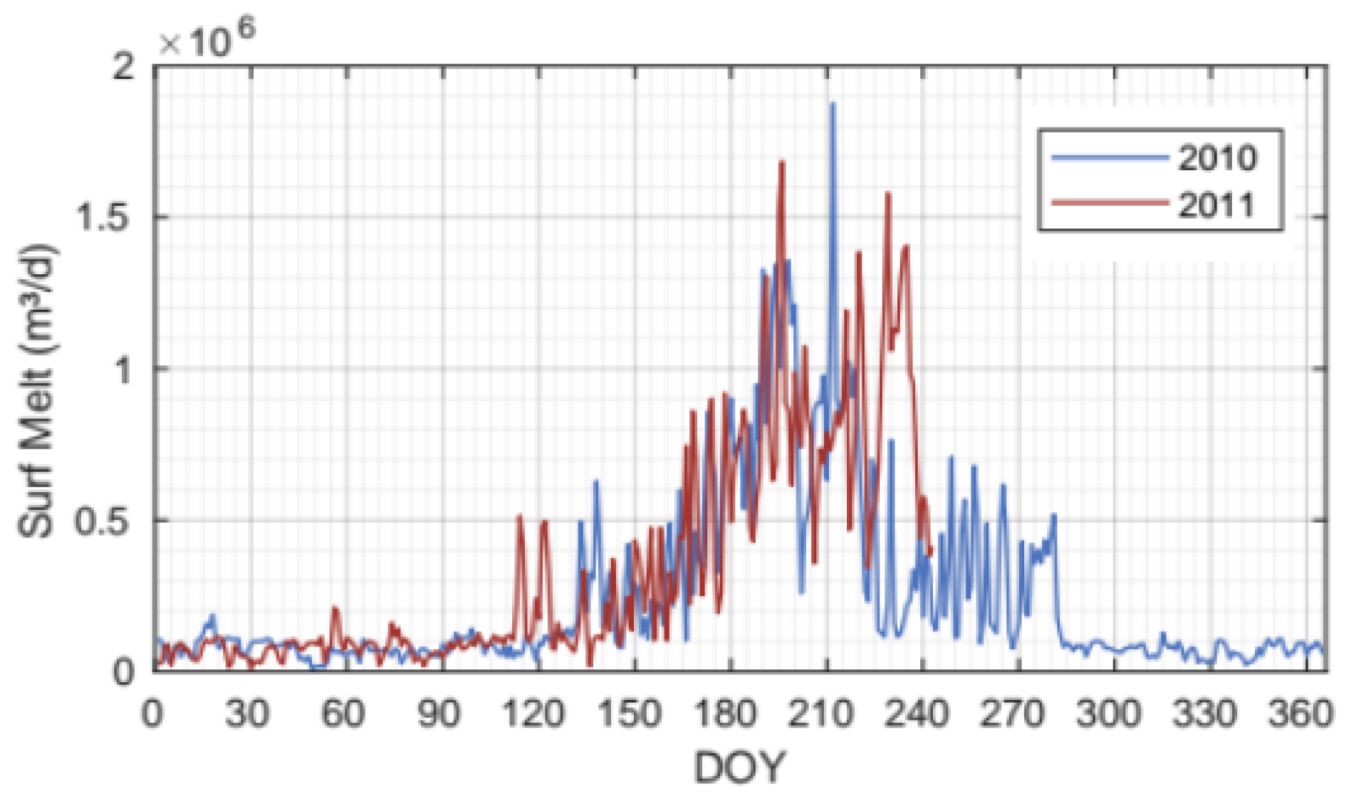
2.2. Observations
2.3. The Models
2.3.1. Glacier Dynamics + Calving
2.3.2. Buoyant Plume + Submarine Melting
2.3.3. Subglacial Hydrology
2.4. Experiments
- Model 1 is coupled with the subglacial hydrology model, allowing meltwater to flow freely through the discharge channels derived from the simulation. This approach enables a more realistic representation of the interactions between the glacier dynamics and the underlying hydrological system.
- Model 2 does not resolve the subglacial hydrology component. Instead, it imposes a single discharge channel, centered along the glacier’s flow line, with an approximate width of 200 m, as described by [17,52]. With this ‘conventional’ configuration, we tested the impact of simplifying subglacial hydrology on the overall dynamics of the glacier–fjord system.
3. Results
3.1. Discharging Channels from the Subglacial Hydrology Model
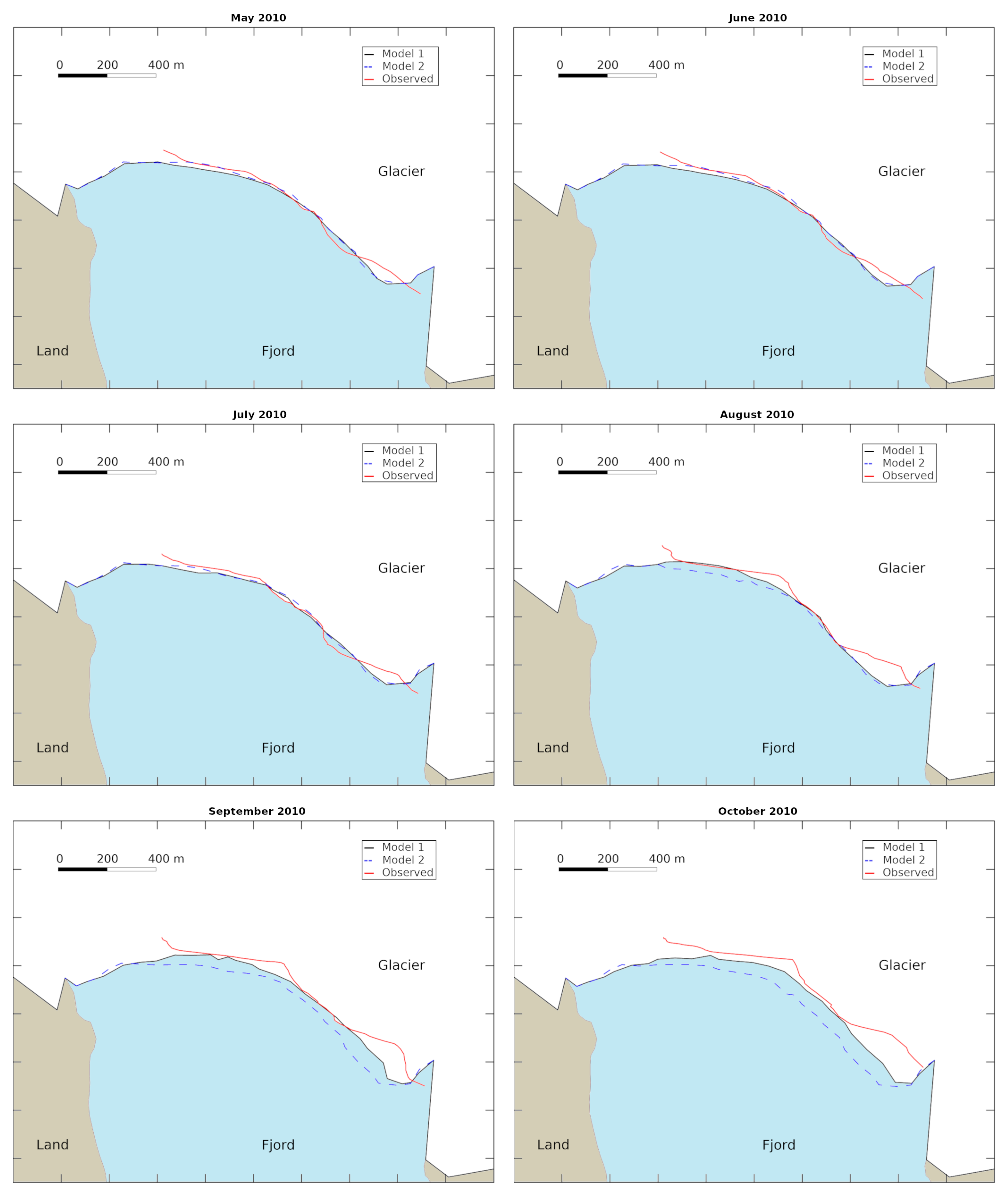
3.2. Performance of the Two Models Against Observed Glacier Terminus
3.3. Comparison of Frontal Ablation Between the Two Models
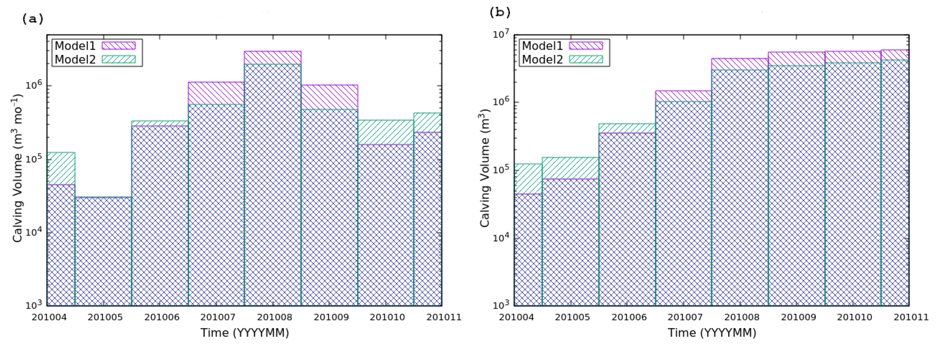
3.3.1. Calving
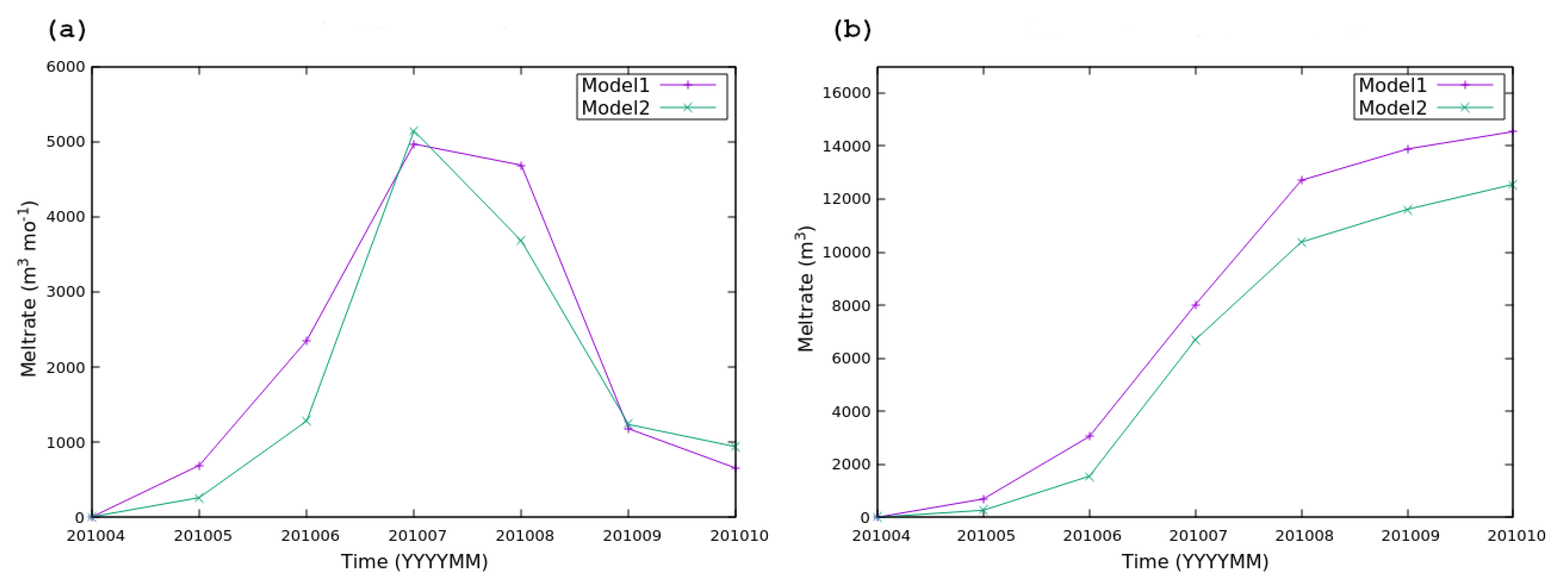
3.3.2. Submarine Melting
4. Discussion
4.1. Subglacial Hydrology as an Important Component of the Glacier–Fjord System
4.2. Implications of Simplifying the Subglacial Hydrology Component in the Modeling Context
5. Conclusions
Author Contributions
Funding
Data Availability Statement
Acknowledgments
Conflicts of Interest
References
- Tesi, T.; Muschitiello, F.; Mollenhauer, G.; Miserocchi, S.; Langone, L.; Ceccarelli, C.; Panieri, G.; Chiggiato, J.; Nogarotto, A.; Hefter, J.; et al. Rapid Atlantification along the Fram Strait at the beginning of the 20th century. Sci. Adv. 2021, 7, eabj2946. [Google Scholar] [CrossRef] [PubMed]
- Strzelewicz, A.; Przyborska, A.; Walczowski, W. Increased presence of Atlantic Water on the shelf south-west of Spitsbergen with implications for the Arctic fjord Hornsund. Prog. Oceanogr. 2022, 200, 102714. [Google Scholar] [CrossRef]
- Tepes, P.; Gourmelen, N.; Nienow, P.; Tsamados, M.; Shepherd, A.; Weissgerber, F. Changes in elevation and mass of Arctic glaciers and ice caps, 2010–2017. Remote Sens. Environ. 2021, 261, 112481. [Google Scholar] [CrossRef]
- Tepes, P.; Nienow, P.; Gourmelen, N. Accelerating Ice Mass Loss Across Arctic Russia in Response to Atmospheric Warming, Sea Ice Decline, and Atlantification of the Eurasian Arctic Shelf Seas. J. Geophys. Res. Earth Surf. 2021, 126, 1–21. [Google Scholar] [CrossRef]
- Hock, R.; Huss, M. Glaciers and climate change. In Climate Change; Elsevier: Amsterdam, The Netherlands, 2021; pp. 157–176. [Google Scholar] [CrossRef]
- Nuth, C.; Gilbert, A.; Köhler, A.; McNabb, R.; Schellenberger, T.; Sevestre, H.; Weidle, C.; Girod, L.; Luckman, A.; Kääb, A. Dynamic vulnerability revealed in the collapse of an Arctic tidewater glacier. Sci. Rep. 2019, 9, 5541. [Google Scholar] [CrossRef]
- Luckman, A.; Benn, D.I.; Cottier, F.; Bevan, S.; Nilsen, F.; Inall, M. Calving rates at tidewater glaciers vary strongly with ocean temperature. Nat. Commun. 2015, 6, 8566. [Google Scholar] [CrossRef]
- Holmes, F.A.; Kirchner, N.; Kuttenkeuler, J.; Krützfeldt, J.; Noormets, R. Relating ocean temperatures to frontal ablation rates at Svalbard tidewater glaciers: Insights from glacier proximal datasets. Sci. Rep. 2019, 9, 9442. [Google Scholar] [CrossRef]
- Błaszczyk, M.; Ignatiuk, D.; Uszczyk, A.; Cielecka-Nowak, K.; Grabiec, M.; Jania, J.A.; Moskalik, M.; Walczowski, W. Freshwater input to the Arctic fjord Hornsund (Svalbard). Polar Res. 2019, 38. [Google Scholar] [CrossRef]
- Cogley, J.G.; Hock, R.; Rasmussen, L.A.; Arendt, A.A.; Bauder, A.; Braithwaite, R.J.; Jansson, P.; Kaser, G.; Möller, M.; Nicholson, L.; et al. Glossary of Glacier Mass Balance and Related Terms; Technical Report, UNESCO-IHP; IACS: Paris, France, 2011. [Google Scholar]
- Huss, M.; Hock, R. A new model for global glacier change and sea-level rise. Front. Earth Sci. 2015, 3, 54. [Google Scholar] [CrossRef]
- Hanna, E.; Pattyn, F.; Navarro, F.; Favier, V.; Goelzer, H.; van den Broeke, M.R.; Vizcaino, M.; Whitehouse, P.L.; Ritz, C.; Bulthuis, K.; et al. Mass balance of the ice sheets and glaciers—Progress since AR5 and challenges. Earth-Sci. Rev. 2020, 201, 102976. [Google Scholar] [CrossRef]
- Mankoff, K.D.; Straneo, F.; Cenedese, C.; Das, S.B.; Richards, C.G.; Singh, H. Structure and dynamics of a subglacial discharge plume in a Greenlandic fjord. J. Geophys. Res. Oceans 2016, 121, 8670–8688. [Google Scholar] [CrossRef]
- De Andrés, E.; Slater, D.; Straneo, F.; Otero, J.; Das, S.; Navarro, F. Surface emergence of glacial plumes determined by fjord stratification. Cryosphere 2020, 14, 1951–1969. [Google Scholar] [CrossRef]
- How, P.; Benn, D.I.; Hulton, N.R.J.; Hubbard, B.; Luckman, A.; Sevestre, H.; van Pelt, W.J.J.; Lindbäck, K.; Kohler, J.; Boot, W. Rapidly changing subglacial hydrological pathways at a tidewater glacier revealed through simultaneous observations of water pressure, supraglacial lakes, meltwater plumes and surface velocities. Cryosphere 2017, 11, 2691–2710. [Google Scholar] [CrossRef]
- Motyka, R.J.; Dryer, W.P.; Amundson, J.; Truffer, M.; Fahnestock, M. Rapid submarine melting driven by subglacial discharge, LeConte Glacier, Alaska. Geophys. Res. Lett. 2013, 40, 5153–5158. [Google Scholar] [CrossRef]
- De Andrés, E.; Otero, J.; Navarro, F.; Promińska, A.; Lapazaran, J.; Walczowski, W. A two-dimensional glacier–fjord coupled model applied to estimate submarine melt rates and front position changes of Hansbreen, Svalbard. J. Glaciol. 2018, 64, 745–758. [Google Scholar] [CrossRef]
- Straneo, F.; Cenedese, C. The Dynamics of Greenland’s Glacial Fjords and Their Role in Climate. Annu. Rev. Mar. Sci. 2015, 7, 89–112. [Google Scholar] [CrossRef]
- Sciascia, R.; Straneo, F.; Cenedese, C.; Heimbach, P. Seasonal variability of submarine melt rate and circulation in an East Greenland fjord. J. Geophys. Res. Oceans 2013, 118, 2492–2506. [Google Scholar] [CrossRef]
- Xu, Y.; Rignot, E.; Fenty, I.; Menemenlis, D.; Flexas, M.M. Subaqueous melting of Store Glacier, west Greenland from three-dimensional, high-resolution numerical modeling and ocean observations. Geophys. Res. Lett. 2013, 40, 4648–4653. [Google Scholar] [CrossRef]
- Slater, D.A.; Nienow, P.W.; Cowton, T.R.; Goldberg, D.N.; Sole, A.J. Effect of near-terminus subglacial hydrology on tidewater glacier submarine melt rates. Geophys. Res. Lett. 2015, 42, 2861–2868. [Google Scholar] [CrossRef]
- Slater, D.A.; Straneo, F.; Das, S.B.; Richards, C.G.; Wagner, T.J.W.; Nienow, P.W. Localized Plumes Drive Front-Wide Ocean Melting of A Greenlandic Tidewater Glacier. Geophys. Res. Lett. 2018, 45, 12350–12358. [Google Scholar] [CrossRef]
- Jackson, R.H.; Motyka, R.J.; Amundson, J.M.; Abib, N.; Sutherland, D.A.; Nash, J.D.; Kienholz, C. The Relationship Between Submarine Melt and Subglacial Discharge From Observations at a Tidewater Glacier. J. Geophys. Res. Oceans 2022, 127, e2021JC018204. [Google Scholar] [CrossRef]
- O’Leary, M.; Christoffersen, P. Calving on tidewater glaciers amplified by submarine frontal melting. Cryosphere 2013, 7, 119–128. [Google Scholar] [CrossRef]
- Vallot, D.; Adinugroho, S.; Strand, R.; How, P.; Pettersson, R.; Benn, D.I.; Hulton, N.R.J. Automatic detection of calving events from time-lapse imagery at Tunabreen, Svalbard. Geosci. Instrum. Methods Data Syst. 2019, 8, 113–127. [Google Scholar] [CrossRef]
- Schild, K.M.; Renshaw, C.E.; Benn, D.I.; Luckman, A.; Hawley, R.L.; How, P.; Trusel, L.; Cottier, F.R.; Pramanik, A.; Hulton, N.R.J. Glacier Calving Rates Due to Subglacial Discharge, Fjord Circulation, and Free Convection. J. Geophys. Res. Earth Surf. 2018, 123, 2189–2204. [Google Scholar] [CrossRef]
- Holmes, F.A.; van Dongen, E.; Kirchner, N. Modelled frontal ablation and velocities at Kronebreen, Svalbard, are sensitive to the choice of submarine melt rate scenario. J. Glaciol. 2023, 1–12. [Google Scholar] [CrossRef]
- Fried, M.J.; Catania, G.A.; Bartholomaus, T.C.; Duncan, D.; Davis, M.; Stearns, L.A.; Nash, J.; Shroyer, E.; Sutherland, D. Distributed subglacial discharge drives significant submarine melt at a Greenland tidewater glacier. Geophys. Res. Lett. 2015, 42, 9328–9336. [Google Scholar] [CrossRef]
- Fried, M.J.; Carroll, D.; Catania, G.A.; Sutherland, D.A.; Stearns, L.A.; Shroyer, E.L.; Nash, J.D. Distinct Frontal Ablation Processes Drive Heterogeneous Submarine Terminus Morphology. Geophys. Res. Lett. 2019, 46, 12083–12091. [Google Scholar] [CrossRef]
- Sutherland, D.A.; Jackson, R.H.; Kienholz, C.; Amundson, J.M.; Dryer, W.P.; Duncan, D.; Eidam, E.F.; Motyka, R.J.; Nash, J.D. Direct observations of submarine melt and subsurface geometry at a tidewater glacier. Science 2019, 365, 369–374. [Google Scholar] [CrossRef]
- Bunce, C.; Nienow, P.; Sole, A.; Cowton, T.; Davison, B. Influence of glacier runoff and near-terminus subglacial hydrology on frontal ablation at a large Greenlandic tidewater glacier. J. Glaciol. 2021, 67, 343–352. [Google Scholar] [CrossRef]
- Bartholomew, I.; Nienow, P.; Sole, A.; Mair, D.; Cowton, T.; King, M.A. Short-term variability in Greenland Ice Sheet motion forced by time-varying meltwater drainage: Implications for the relationship between subglacial drainage system behavior and ice velocity. J. Geophys. Res. Earth Surf. 2012, 117, 1–17. [Google Scholar] [CrossRef]
- Bell, R.E. The role of subglacial water in ice-sheet mass balance. Nat. Geosci. 2008, 1, 297–304. [Google Scholar] [CrossRef]
- Zwally, H.J.; Abdalati, W.; Herring, T.; Larson, K.; Saba, J.; Steffen, K. Surface Melt-Induced Acceleration of Greenland Ice-Sheet Flow. Science 2002, 297, 218–222. [Google Scholar] [CrossRef] [PubMed]
- van de Wal, R.S.W.; Boot, W.; van den Broeke, M.R.; Smeets, C.J.P.P.; Reijmer, C.H.; Donker, J.J.A.; Oerlemans, J. Large and Rapid Melt-Induced Velocity Changes in the Ablation Zone of the Greenland Ice Sheet. Science 2008, 321, 111–113. [Google Scholar] [CrossRef] [PubMed]
- Cowton, T.; Nienow, P.; Sole, A.; Wadham, J.; Lis, G.; Bartholomew, I.; Mair, D.; Chandler, D. Evolution of drainage system morphology at a land-terminating Greenlandic outlet glacier. J. Geophys. Res. Earth Surf. 2013, 118, 29–41. [Google Scholar] [CrossRef]
- Fountain, A.G.; Walder, J.S. Water flow through temperate glaciers. Rev. Geophys. 1998, 36, 299–328. [Google Scholar] [CrossRef]
- Nienow, P.; Sharp, M.; Willis, I. Seasonal changes in the morphology of the subglacial drainage system, Haut Glacier d’Arolla, Switzerland. Earth Surf. Process. Landf. 1998, 23, 825–843. [Google Scholar] [CrossRef]
- Weertman, J. General theory of water flow at the base of a glacier or ice sheet. Rev. Geophys. 1972, 10, 287–333. [Google Scholar] [CrossRef]
- Hodgkins, R. Glacier hydrology in Svalbard, Norwegian high arctic. Quat. Sci. Rev. 1997, 16, 957–973. [Google Scholar] [CrossRef]
- Decaux, L.; Grabiec, M.; Ignatiuk, D.; Jania, J. Role of discrete water recharge from supraglacial drainage systems in modeling patterns of subglacial conduits in Svalbard glaciers. Cryosphere 2019, 13, 735–752. [Google Scholar] [CrossRef]
- Flowers, G.E. Modelling water flow under glaciers and ice sheets. Proc. R. Soc. A Math. Phys. Eng. Sci. 2015, 471, 20140907. [Google Scholar] [CrossRef]
- Kamb, B.; Raymond, C.F.; Harrison, W.D.; Engelhardt, H.; Echelmeyer, K.A.; Humphrey, N.; Brugman, M.M.; Pfeffer, T. Glacier Surge Mechanism: 1982-1983 Surge of Variegated Glacier, Alaska. Science 1985, 227, 469–479. [Google Scholar] [CrossRef] [PubMed]
- Kamb, B. Glacier surge mechanism based on linked cavity configuration of the basal water conduit system. J. Geophys. Res. Solid Earth 1987, 92, 9083–9100. [Google Scholar] [CrossRef]
- Muñoz-Hermosilla, J.M.; Otero, J.; De Andrés, E.; Shahateet, K.; Navarro, F.; Pérez-Doña, I. A 3D glacier dynamics–line plume model to estimate the frontal ablation of Hansbreen, Svalbard. Cryosphere 2024, 18, 1911–1924. [Google Scholar] [CrossRef]
- Cook, S.J.; Christoffersen, P.; Todd, J.; Slater, D.; Chauché, N. Coupled modelling of subglacial hydrology and calving-front melting at Store Glacier, West Greenland. Cryosphere 2020, 14, 905–924. [Google Scholar] [CrossRef]
- Cook, S.J.; Christoffersen, P.; Todd, J. A fully-coupled 3D model of a large Greenlandic outlet glacier with evolving subglacial hydrology, frontal plume melting and calving. J. Glaciol. 2022, 68, 486–502. [Google Scholar] [CrossRef]
- Möller, M.; Navarro, F.; Huss, M.; Marzeion, B. Projected sea-level contributions from tidewater glaciers are highly sensitive to chosen bedrock topography: A case study at Hansbreen, Svalbard. J. Glaciol. 2023, 69, 966–980. [Google Scholar] [CrossRef]
- Grabiec, M.; Jania, J.A.; Puczko, D.; Kolondra, L.; Budzik, T. Surface and bed morphology of Hansbreen, a tidewater glacier in Spitsbergen. Pol. Polar Res. 2012, 33, 111–138. [Google Scholar] [CrossRef]
- Błaszczyk, M.; Jania, J.A.; Ciepły, M.; Grabiec, M.; Ignatiuk, D.; Kolondra, L.; Kruss, A.; Luks, B.; Moskalik, M.; Pastusiak, T.; et al. Factors Controlling Terminus Position of Hansbreen, a Tidewater Glacier in Svalbard. J. Geophys. Res. Earth Surf. 2021, 126, 1–20. [Google Scholar] [CrossRef]
- Ćwia̧kała, J.; Moskalik, M.; Forwick, M.; Wojtysiak, K.; Giżejewski, J.; Szczuciński, W. Submarine geomorphology at the front of the retreating Hansbreen tidewater glacier, Hornsund fjord, southwest Spitsbergen. J. Maps 2018, 14, 123–134. [Google Scholar] [CrossRef]
- De Andrés, E.; Otero, J.; Navarro, F.J.; Walczowski, W. Glacier–plume or glacier–fjord circulation models? A 2-D comparison for Hansbreen–Hansbukta system, Svalbard. J. Glaciol. 2021, 67, 797–810. [Google Scholar] [CrossRef]
- Perez-Doña, I.; Otero, J. Sobre el uso de Kriging Bayesiano para estimar la evolución de las velocidades en superficie del Glaciar Hansbreen (Svalbard). In Proceedings of the 10a Asamblea Hispano-Portuguesa de Geodesia y Geofísica, Toledo, Spain, 28 November–1 September 2023. [Google Scholar]
- Finkelnburg, R. Climate Variability of Svalbard in the First Decade of the 21st Century and Its Impact on Vestfonna Ice Cap, Nordaustlandet. Ph.D. Thesis, Technischen Universität Berlin, Berlin, Germany, 2013. [Google Scholar] [CrossRef]
- Navarro, F.J.; Martín-Español, A.; Lapazaran, J.J.; Grabiec, M.; Otero, J.; Vasilenko, E.V.; Puczko, D. Ice Volume Estimates from Ground-Penetrating Radar Surveys, Wedel Jarlsberg Land Glaciers, Svalbard. Arct. Antarct. Alp. Res. 2014, 46, 394–406. [Google Scholar] [CrossRef]
- Otero, J.; Navarro, F.J.; Lapazaran, J.J.; Welty, E.; Puczko, D.; Finkelnburg, R. Modeling the Controls on the Front Position of a Tidewater Glacier in Svalbard. Front. Earth Sci. 2017, 5, 1–11. [Google Scholar] [CrossRef]
- Gagliardini, O.; Zwinger, T.; Gillet-Chaulet, F.; Durand, G.; Favier, L.; de Fleurian, B.; Greve, R.; Malinen, M.; Martín, C.; Råback, P.; et al. Capabilities and performance of Elmer/Ice, a new-generation ice sheet model. Geosci. Model Dev. 2013, 6, 1299–1318. [Google Scholar] [CrossRef]
- Cuffey, K.; Paterson, W. The Physics of Glaciers, 4th ed.; Elsevier: Oxford, UK, 2010. [Google Scholar]
- Todd, J.; Christoffersen, P.; Zwinger, T.; Råback, P.; Chauché, N.; Benn, D.; Luckman, A.; Ryan, J.; Toberg, N.; Slater, D.; et al. A Full-Stokes 3-D Calving Model Applied to a Large Greenlandic Glacier. J. Geophys. Res. Earth Surf. 2018, 123, 410–432. [Google Scholar] [CrossRef]
- Todd, J.; Christoffersen, P.; Zwinger, T.; Råback, P.; Benn, D.I. Sensitivity of a calving glacier to ice–ocean interactions under climate change: New insights from a 3-D full-Stokes model. Cryosphere 2019, 13, 1681–1694. [Google Scholar] [CrossRef]
- Benn, D.I.; Hulton, N.R.; Mottram, R.H. ‘Calving laws’, ‘sliding laws’ and the stability of tidewater glaciers. Ann. Glaciol. 2007, 46, 123–130. [Google Scholar] [CrossRef]
- Nick, F.; Van der Veen, C.; Vieli, A.; Benn, D. A physically based calving model applied to marine outlet glaciers and implications for the glacier dynamics. J. Glaciol. 2010, 56, 781–794. [Google Scholar] [CrossRef]
- Otero, J.; Navarro, F.J.; Martin, C.; Cuadrado, M.L.; Corcuera, M.I. A three-dimensional calving model: Numerical experiments on Johnsons Glacier, Livingston Island, Antarctica. J. Glaciol. 2010, 56, 200–214. [Google Scholar] [CrossRef]
- Todd, J.; Christoffersen, P. Are seasonal calving dynamics forced by buttressing from ice mélange or undercutting by melting? Outcomes from full-Stokes simulations of Store Glacier, West Greenland. Cryosphere 2014, 8, 2353–2365. [Google Scholar] [CrossRef]
- Benn, D.I.; Todd, J.; Luckman, A.; Bevan, S.; Chudley, T.R.; Åström, J.; Zwinger, T.; Cook, S.; Christoffersen, P. Controls on calving at a large Greenland tidewater glacier: Stress regime, self-organised criticality and the crevasse-depth calving law. J. Glaciol. 2023, 1–16. [Google Scholar] [CrossRef]
- Jenkins, A. Convection-driven melting near the grounding lines of ice shelves and tidewater glaciers. J. Phys. Oceanogr. 2011, 41, 2279–2294. [Google Scholar] [CrossRef]
- Jackson, R.H.; Shroyer, E.L.; Nash, J.D.; Sutherland, D.A.; Carroll, D.; Fried, M.J.; Catania, G.A.; Bartholomaus, T.C.; Stearns, L.A. Near-glacier surveying of a subglacial discharge plume: Implications for plume parameterizations. Geophys. Res. Lett. 2017, 44, 6886–6894. [Google Scholar] [CrossRef]
- Holland, D.M.; Jenkins, A. Modeling Thermodynamic Ice–Ocean Interactions at the Base of an Ice Shelf. J. Phys. Oceanogr. 1999, 29, 1787–1800. [Google Scholar] [CrossRef]
- Gagliardini, O.; Werder, M.A. Influence of increasing surface melt over decadal timescales on land-terminating Greenland-type outlet glaciers. J. Glaciol. 2018, 64, 700–710. [Google Scholar] [CrossRef]
- Werder, M.A.; Hewitt, I.J.; Schoof, C.G.; Flowers, G.E. Modeling channelized and distributed subglacial drainage in two dimensions. J. Geophys. Res. Earth Surf. 2013, 118, 2140–2158. [Google Scholar] [CrossRef]
- How, P.; Schild, K.M.; Benn, D.I.; Noormets, R.; Kirckner, N.; Luckman, A.; Vallot, D.; Hulton, N.R.J.; Borstad, C. Calving controlled by melt-under-cutting: Detailed calving styles revealed through time-lapse observations. Ann. Glaciol. 2019, 60, 20–31. [Google Scholar] [CrossRef]
- Ma, Y.; Bassis, J.N. The Effect of Submarine Melting on Calving From Marine Terminating Glaciers. J. Geophys. Res. Earth Surf. 2019, 124, 334–346. [Google Scholar] [CrossRef]
- Stevens, L.A.; Straneo, F.; Das, S.B.; Plueddemann, A.J.; Kukulya, A.L.; Morlighem, M. Linking glacially modified waters to catchment-scale subglacial discharge using autonomous underwater vehicle observations. Cryosphere 2016, 10, 417–432. [Google Scholar] [CrossRef]
- Jouvet, G.; Weidmann, Y.; Kneib, M.; Detert, M.; Seguinot, J.; Sakakibara, D.; Sugiyama, S. Short-lived ice speed-up and plume water flow captured by a VTOL UAV give insights into subglacial hydrological system of Bowdoin Glacier. Remote Sens. Environ. 2018, 217, 389–399. [Google Scholar] [CrossRef]
- Cowton, T.R.; Todd, J.A.; Benn, D.I. Sensitivity of Tidewater Glaciers to Submarine Melting Governed by Plume Locations. Geophys. Res. Lett. 2019, 46, 11219–11227. [Google Scholar] [CrossRef]
- Carroll, D.; Sutherland, D.A.; Hudson, B.; Moon, T.; Catania, G.A.; Shroyer, E.L.; Nash, J.D.; Bartholomaus, T.C.; Felikson, D.; Stearns, L.A.; et al. The impact of glacier geometry on meltwater plume structure and submarine melt in Greenland fjords. Geophys. Res. Lett. 2016, 43, 9739–9748. [Google Scholar] [CrossRef]
- Nick, F.; Oerlemans, J. Dynamics of tidewater glaciers: Comparison of three models. J. Glaciol. 2006, 52, 183–190. [Google Scholar] [CrossRef]
- Amundson, J.M.; Truffer, M.; Zwinger, T. Tidewater glacier response to individual calving events. J. Glaciol. 2022, 68, 1117–1126. [Google Scholar] [CrossRef]
- Umlauft, J.; Johnson, C.W.; Roux, P.; Trugman, D.T.; Lecointre, A.; Walpersdorf, A.; Nanni, U.; Gimbert, F.; Rouet-Leduc, B.; Hulbert, C.; et al. Mapping Glacier Basal Sliding Applying Machine Learning. J. Geophys. Res. Earth Surf. 2023, 128, e2023JF007280. [Google Scholar] [CrossRef]
- Prieur, C.; Rabatel, A.; Thomas, J.B.; Farup, I.; Chanussot, J. Machine Learning Approaches to Automatically Detect Glacier Snow Lines on Multi-Spectral Satellite Images. Remote Sens. 2022, 14, 3868. [Google Scholar] [CrossRef]
- Gogineni, A.; Chintalacheruvu, M.R.; Kale, R.V. Modelling of snow and glacier melt dynamics in a mountainous river basin using integrated SWAT and machine learning approaches. Earth Sci. Inform. 2024, 17, 4315–4337. [Google Scholar] [CrossRef]
- Bolibar, J.; Rabatel, A.; Gouttevin, I.; Galiez, C.; Condom, T.; Sauquet, E. Deep learning applied to glacier evolution modelling. Cryosphere 2020, 14, 565–584. [Google Scholar] [CrossRef]
- Bolibar, J.; Rabatel, A.; Gouttevin, I.; Zekollari, H.; Galiez, C. Nonlinear sensitivity of glacier mass balance to future climate change unveiled by deep learning. Nat. Commun. 2022, 13, 409. [Google Scholar] [CrossRef]
- Ren, W.; Zhu, Z.; Wang, Y.; Su, J.; Zeng, R.; Zheng, D.; Li, X. Comparison of Machine Learning Models in Simulating Glacier Mass Balance: Insights from Maritime and Continental Glaciers in High Mountain Asia. Remote Sens. 2024, 16, 956. [Google Scholar] [CrossRef]


| Description | Name | Value | Units |
|---|---|---|---|
| Pressure melt coefficient | 7.5 × 10⁻⁸ | KPa−1 | |
| Heat capacity of water | 4220 | J kg−1K−1 | |
| Sheet flow exponent | 3 | ||
| Sheet flow exponent | 2 | ||
| Channel flow exponent | 5/4 | ||
| Channel flow exponent | 3/2 | ||
| Sheet conductivity | 0.005 | m s−1kg−1 | |
| Channel conductivity | 0.1 | m3/2kg−1/2 | |
| Sheet width below channel | 0.2 | m | |
| Cavity spacing | 0.5 | m | |
| Bedrock bump ratio | 0.02 | m | |
| Englacial void ratio | 10−4 |
| Date | Model 1 | Model 2 |
|---|---|---|
| (mmmYYYY) | Longitudinal Difference (m) | Longitudinal Difference (m) |
| April 2010 | 0.77 | −0.03 |
| May 2010 | −3.72 | 1.53 |
| June 2010 | −4.8 | 3.91 |
| July 2010 | 13.42 | 31.97 |
| August 2010 | 30.47 | 64.7 |
| September 2010 | 53.78 | 100.22 |
| October 2010 | 75.99 | 121.9 |
Disclaimer/Publisher’s Note: The statements, opinions and data contained in all publications are solely those of the individual author(s) and contributor(s) and not of MDPI and/or the editor(s). MDPI and/or the editor(s) disclaim responsibility for any injury to people or property resulting from any ideas, methods, instructions or products referred to in the content. |
© 2024 by the authors. Licensee MDPI, Basel, Switzerland. This article is an open access article distributed under the terms and conditions of the Creative Commons Attribution (CC BY) license (https://creativecommons.org/licenses/by/4.0/).
Share and Cite
De Andrés, E.; Muñoz-Hermosilla, J.M.; Shahateet, K.; Otero, J. The Importance of Solving Subglaciar Hydrology in Modeling Glacier Retreat: A Case Study of Hansbreen, Svalbard. Hydrology 2024, 11, 193. https://doi.org/10.3390/hydrology11110193
De Andrés E, Muñoz-Hermosilla JM, Shahateet K, Otero J. The Importance of Solving Subglaciar Hydrology in Modeling Glacier Retreat: A Case Study of Hansbreen, Svalbard. Hydrology. 2024; 11(11):193. https://doi.org/10.3390/hydrology11110193
Chicago/Turabian StyleDe Andrés, Eva, José M. Muñoz-Hermosilla, Kaian Shahateet, and Jaime Otero. 2024. "The Importance of Solving Subglaciar Hydrology in Modeling Glacier Retreat: A Case Study of Hansbreen, Svalbard" Hydrology 11, no. 11: 193. https://doi.org/10.3390/hydrology11110193
APA StyleDe Andrés, E., Muñoz-Hermosilla, J. M., Shahateet, K., & Otero, J. (2024). The Importance of Solving Subglaciar Hydrology in Modeling Glacier Retreat: A Case Study of Hansbreen, Svalbard. Hydrology, 11(11), 193. https://doi.org/10.3390/hydrology11110193