A Silhouette-Width-Induced Hierarchical Clustering for Defining Flood Estimation Regions

Abstract

Flood quantile estimation in ungauged basins is often performed using regional analysis. A regionalization procedure consists of two phases: the definition of homogeneous regions among gauged basins, i.e., clusters of stations, and information transfer to the ungauged sites. Due to its simplicity and widespread use, a combination of hierarchical clustering by Ward’s algorithm and the index-flood method is applied in this research. While hierarchical clustering is very efficient, its shortcomings are the lack of flexibility in the definition of clusters/regions and the inability to transfer objects/stations from one cluster center to another. To overcome this, using silhouette width for induced clustering of stations in flood studies is proposed in this paper. A regionalization procedure is conducted on 53 gauging stations under a continental climate in the West Balkans. In the induced clustering, a negative silhouette width is used as an indicator for the relocation of station(s) to another cluster. The estimates of mean annual flood and 100-year flood quantiles assessed by the original and induced clustering are compared. A jackknife procedure is applied for mean annual flood estimation and 100-year flood quantiles. Both the Hosking–Wallis and Anderson–Darling bootstrap tests provide better results regarding the homogeneity of the defined regions for the induced clustering compared to the original one. The goodness-of-fit measures indicate improved clustering results by the proposed intervention, reflecting flood quantile estimation at the stations with significant overestimation by the original clustering.

1. Introduction

Flood frequency analysis (FFA) is commonly used in hydrology to relate extreme river flow to its frequency of occurrence, i.e., to estimate flood quantile [1]. The application of statistical methods in this analysis implies long-term, reliable gauge flow data [2]. For instance, a known issue with gauged high flows is the uncertainty of the rating curve that provides the relationship between the water flow and the corresponding water stage in that particular domain of interest [3,4]. The application of statistical methods implies homogeneous and stationary datasets, which contradicts the increasing evidence for climate change [5,6], although some flood-related studies suggest the opposite [7,8,9,10]. Assuming that the datasets are homogeneous and reliable, the next question is whether the population distribution function and its parameters can be reliably estimated from the available data record length.

Some countries have suggested procedures, distribution functions, and parameter estimation methods for FFA. In the USA, the Log Pearson 3 (LP3) function is used, with the parameters estimated by the expected moments algorithm (EMA) [11]; in the Russian Federation, either Kritsky–Menkel, Pearson 3 or Log Normal distribution is used, depending on the ratio of the skew (Cs) and coefficient of variation (Cv), with the use of the approximate method of maximum likelihood (MLE) [12], while in Germany, the choice of distribution function depends on the data record length [13]. The use of three-parameter distributions in Germany is allowed for data records that are at least 50 years long. In addition, MLE, the method of ordinary moments and L-moments are used to estimate the distribution parameters, without preference. It is assumed that all methods lead to approximately equal results, and if this is not the case, it is necessary to include other information. In general, such inclusion is conducted with the temporal, spatial, and causal expansion of information used for the improvement of flood quantile estimation [14,15].

Spatial data transfer, in the focus of this research, includes methods of regionalization for estimating parameters or flood quantiles. It is most often used when the data record is short or completely absent (ungauged catchment/site). The spatial information expansion includes spatial regionalization and statistical regionalization. Spatial regionalizations imply the creation of envelope curves, specific runoff diagrams [13], maps of quantiles or maps of a certain statistical parameter. Envelope curves and specific runoff diagrams show high flows in relation to the catchment area or a section of the river network and serve to verify the estimated peak flows. The extrapolation of envelope curves for areas outside the observation range is problematic [13].

Statistical regionalization procedures imply the determination of the relationship between the parameters/quantiles of high-flows and the morphological and/or meteorological parameters of the catchment. When the flow data record is shorter than half of the required return period, regional statistics can help to improve the dataset statistics [13]. In statistical regionalization procedures, two steps are crucial: the formation of homogeneous regions and the transfer of information, that is, the flood flow estimation. Many regionalization methods have been recommended in the literature, and the difference between them is in these two steps.

Assuming that similar processes take place in areas that are physically close to each other, geographically continuous regions are often considered homogeneous regions for flood flow estimation. This approach is subjective because neighboring areas do not always behave in a hydrologically similar way [16]; hence, cluster methods [17,18,19] or the Region of Influence (ROI) method [20,21] are used.

In the ROI and cluster analyses, it is necessary to select similarity attributes for grouping (regionalizing) catchments. Given that they are easily available, geomorphological properties are most often used [22,23], then hydro-meteorological properties [24,25] or seasonality of peak flows [26,27], which has the advantage of high accuracy and robustness of the data, dates of occurrence of peak flows, form of distribution [27,28], etc.

Due to its practicality, the use of cluster analysis in flood regionalization is frequent [17,18]. Most often, clustering is performed using Ward’s algorithm (hierarchical approach) [26,29] or the k-means algorithm (partition approach) [30,31]. The advantage of the hierarchical approach is in the way the results are presented (dendrogram), from which regions can be determined for an arbitrary distance or number of cluster centers (CCs). In the partition approach, this is not possible, but the number of CCs has to be specified in advance. As the result may depend on the initially assumed CCs, the algorithm needs to be run several times. Due to the hierarchic approach, it happens that the object (catchment) assigned to the CC at an early stage is found to be inadequate after the formation of the CC/region [17]. The fact that objects cannot migrate from one CC to another is the shortcoming of a hierarchical approach. To take advantage of both clustering methods, a hybrid cluster analysis [18] was proposed, which implies a hierarchical approach in the first step, and then its result represents the assumed starting CCs for the partition approach in the second step.

In the study area for this research, i.e., Bosnia and Herzegovina, specific runoff diagrams or regression that relates flood quantiles and catchment area are most often used for flood quantile estimation in ungauged catchments [32]. It was shown that this approach can give significant under-/overestimation of flood quantiles and that geographically continuous regions of water basins are considered homogeneous regions without testing [33,34]. Other methods for flood data transfer used to improve flood quantile estimation included an extension of the gauged peak flow data based on gauged water stage, assumed rating curves [35], and historic floods [36]. A comparative presentation of statistical results, empirical expressions, and a geomorphological unit hydrograph using the EBA4SUB model is also considered [37]. Regional analysis using the cluster method was performed for stations from Bosnia and Herzegovina with the addition of stations from Serbia, where the advantage of hierarchical (Ward’s algorithm) over partition (k-means) clustering was demonstrated in flood quantile estimation [33].

In this study, another approach to forming regions for flood quantile estimation is investigated, which is fundamentally hierarchical. The adequacy of assigning objects to CCs is examined through the (mean) silhouette width value [38], which is intended for determining the optimal number of CCs [39] and as a measure of the region compactness [40]. The advantage of silhouette width is that it does not require a training set to evaluate clustering results [41]. Similarly to the k-means algorithm, the proposed procedure also requires an iterative method. The important difference is that the k-means algorithm depends on the assumed initial CCs, while in the proposed method, this is not the case. Based on quantitative measures such as silhouette width, the same input data give a unique result.

The research question is as follows: is silhouette-width-induced clustering of catchments appropriate for the formation of flood estimation regions in a data-scarce environment? This research was conducted for the study region of Bosnia and Herzegovina and Serbia and is based on the findings from the initial study [34]. The appropriateness of the silhouette-width-induced clustering was rated using the performance-based assessment that also included region homogeneity examination and flood information transfer by the index-flood method. The flood quantile estimation procedure for pseudo-ungauged catchments was conducted in the common way used in Bosnia and Herzegovina.

2. Materials and Methods

2.1. Study Region and Data

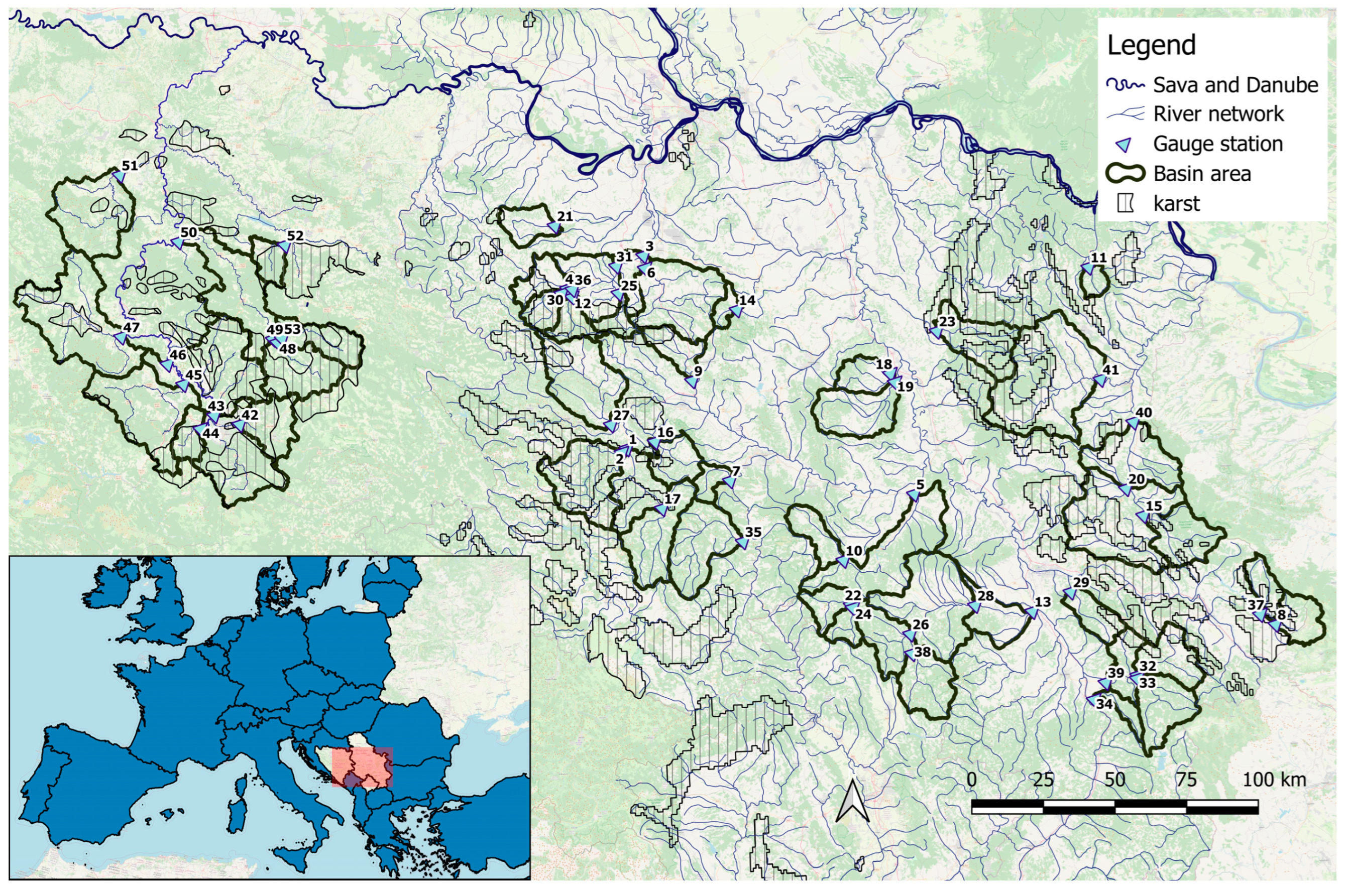
The study region is the southern part of the Danube River basin, characterized by a continental climate. The annual peak flow data were collected for 64 hydrological stations (HSs), with a catchment area of up to 3000 km² in the territory of Bosnia and Herzegovina (19 HSs) and Serbia (45 HSs). The data were quality assured by the respective hydrometeorological services. A total of 11 HSs were excluded from this study due to different reasons, including short peak flow datasets, a flow regime regulated by upstream reservoirs, and difficulty in defining a catchment border due to karst. The locations and catchment boundaries of the remaining 53 HSs are shown in Figure 1.

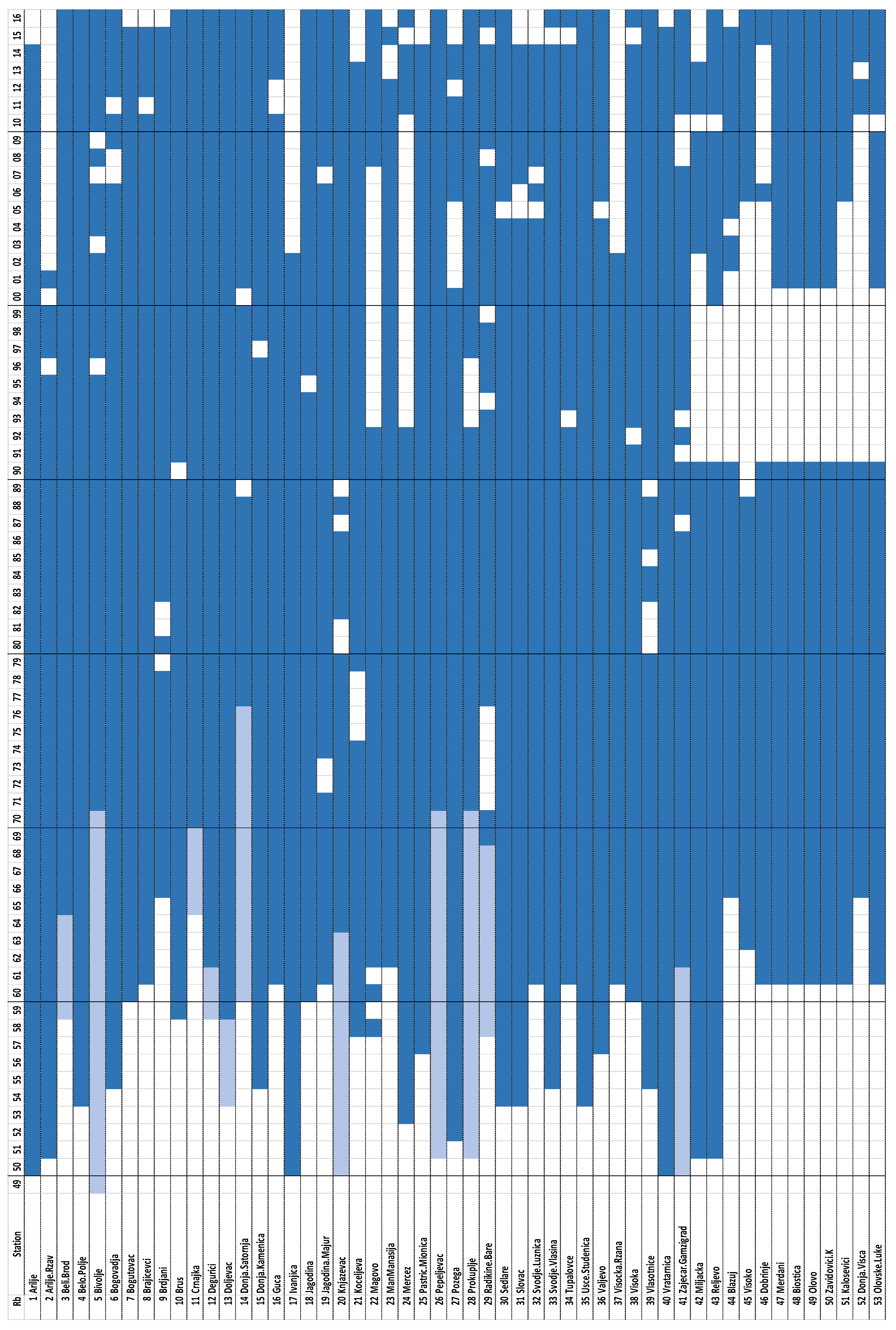
The peak flow datasets of 53 HSs in the gauge period 1948–2016 were subjected to statistical tests to determine suitability for statistical analysis, i.e., flood frequency analysis (tests of stationarity, independence, and homogeneity in mean and variance). In 12 HSs, the datasets were trimmed (cut off) from the beginning of a gauge period until they were found to be suitable for statistical analysis at the 5% significance level of the applied tests. The trimmed gauged peak flow data range is from 1 to 22 years. The completeness and gauge period of the datasets are shown graphically in Appendix A (Figure A1). Long data gaps are characteristic for the HSs in Bosnia and Herzegovina, starting from HS no. 43 in Figure A1. The incomplete datasets were not augmented. The average size of the datasets is 51 years.

Table A1. Annual peak flow dataset statistics.

HS	Station	N	Ntrimm	MAF	S	Cv	Cs	t	t3	t4
1	Arilje	65		120.6	81.0	0.672	1.980	0.308	0.250	0.147
2	Arilje.Rzav	49		100.1	48.9	0.488	1.404	0.256	0.208	0.089
3	Beli.Brod	52	6	288.6	218.0	0.755	2.755	0.345	0.300	0.183
4	Belo.Polje	63		59.7	43.5	0.729	1.823	0.314	0.169	0.105
5	Bivolje	42	22	101.7	72.5	0.713	1.074	0.280	0.083	0.054
6	Bogovadja	59		99.3	86.0	0.865	4.863	0.388	0.391	0.318
7	Bogutovac	56		35.6	31.3	0.878	3.103	0.398	0.263	0.188
8	Brajicevci	54		40.0	26.5	0.661	1.312	0.286	0.153	0.076
9	Brdjani	47		51.6	43.2	0.838	1.839	0.390	0.239	0.092
10	Brus	57		32.6	24.5	0.751	1.912	0.427	0.242	0.105
11	Crnajka	47	5	25.1	25.3	1.012	2.862	0.433	0.327	0.229
12	Degurici	55	3	44.1	32.8	0.744	2.449	0.338	0.254	0.178
13	Doljevac	58	5	135.5	93.4	0.689	1.639	0.335	0.229	0.105
14	Donja.Satornja	38	17	18.8	31.3	1.664	3.459	0.617	0.401	0.276
15	Donja.Kamenica	61		44.2	41.5	0.939	2.977	0.421	0.348	0.237
16	Guca	54		71.2	47.7	0.669	1.701	0.255	0.257	0.149
17	Ivanjica	53		75.5	63.2	0.837	3.803	0.431	0.380	0.253
18	Jagodina	56		19.3	18.0	0.935	2.018	0.407	0.265	0.136
19	Jagodina.Majur	53		73.3	81.0	1.105	2.532	0.457	0.322	0.184
20	Knjazevac	49	14	113.2	68.9	0.609	1.116	0.214	0.155	0.073
21	Koceljeva	52	1	33.5	24.9	0.745	1.744	0.346	0.219	0.083
22	Magovo	42		30.1	34.7	1.155	3.731	0.563	0.461	0.360
23	ManManasija	52		60.9	57.0	0.936	2.213	0.448	0.301	0.156
24	Mercez	45		19.6	19.6	1.004	2.852	0.549	0.382	0.221
25	Pastric.Mionica	58		50.4	69.8	1.385	3.320	0.600	0.398	0.227
26	Pepeljevac	46	20	130.4	89.0	0.682	2.155	0.309	0.239	0.162
27	Pozega	57		118.9	110.6	0.930	2.141	0.377	0.208	0.125
28	Prokuplje	42	20	151.4	122.8	0.811	2.757	0.399	0.349	0.240
29	Radikine.Bare	38	11	23.1	15.5	0.670	0.917	0.251	0.092	−0.038
30	Sedlare	62		41.7	38.4	0.920	1.870	0.419	0.255	0.115
31	Slovac	59		187.9	141.1	0.751	4.834	0.300	0.312	0.241
32	Svodje.Luznica	52		62.9	69.6	1.106	4.673	0.400	0.329	0.274
33	Svodje.Vlasina	61		49.0	59.1	1.205	4.427	0.488	0.416	0.307
34	Tupalovce	54		22.2	12.9	0.582	1.410	0.282	0.178	0.079
35	Usce.Studenica	63		59.2	38.0	0.642	3.507	0.363	0.320	0.197
36	Valjevo	59		85.8	65.3	0.761	2.217	0.335	0.188	0.074
37	Visocka.Rzana	42		69.9	41.6	0.595	1.460	0.298	0.179	0.101
38	Visoka	55		71.2	62.4	0.877	2.454	0.377	0.212	0.141
39	Vlasotnice	57		147.3	125.2	0.850	2.794	0.331	0.256	0.181
40	Vratarnica	66		142.5	77.3	0.543	0.856	0.131	0.148	0.087
41	Zajecar.Gamzigrad	49	12	110.0	66.3	0.603	1.589	0.251	0.212	0.094
42	Miljacka	50		74.3	40.8	0.549	1.295	0.268	0.165	0.062
43	Reljevo	56		239.8	81.5	0.340	0.747	0.110	0.144	0.076
44	Blazuj	38		36.1	18.6	0.516	1.407	0.352	0.145	0.024
45	Visoko	37		146.7	71.0	0.484	0.753	0.199	0.048	0.055
46	Dobrinje	33		398.2	166.9	0.419	1.765	0.233	0.221	0.118
47	Merdani	46		125.6	78.7	0.627	2.930	0.320	0.216	0.141
48	Biostica	46		83.8	56.5	0.674	2.058	0.400	0.280	0.138
49	Olovo	46		166.8	102.2	0.612	1.676	0.315	0.206	0.121
50	Zavidovici.K	46		358.5	173.1	0.483	1.229	0.247	0.158	0.077
51	Kalosevici	41		245.6	130.5	0.531	0.480	0.135	0.029	−0.049
52	Donja.Visca	30		60.1	34.2	0.570	1.506	0.301	0.204	0.113
53	Olovske.Luke	45		81.2	55.9	0.688	1.238	0.319	0.130	0.028

in Appendix A contains the analyzed datasets’ flood statistics for the 53 HSs.

The catchment morphological attributes, catchment area (A), average slope (Iavg) and average elevation (Havg), are taken from previous research, determined from the 20 m resolution DEM [42].

2.2. Methodology

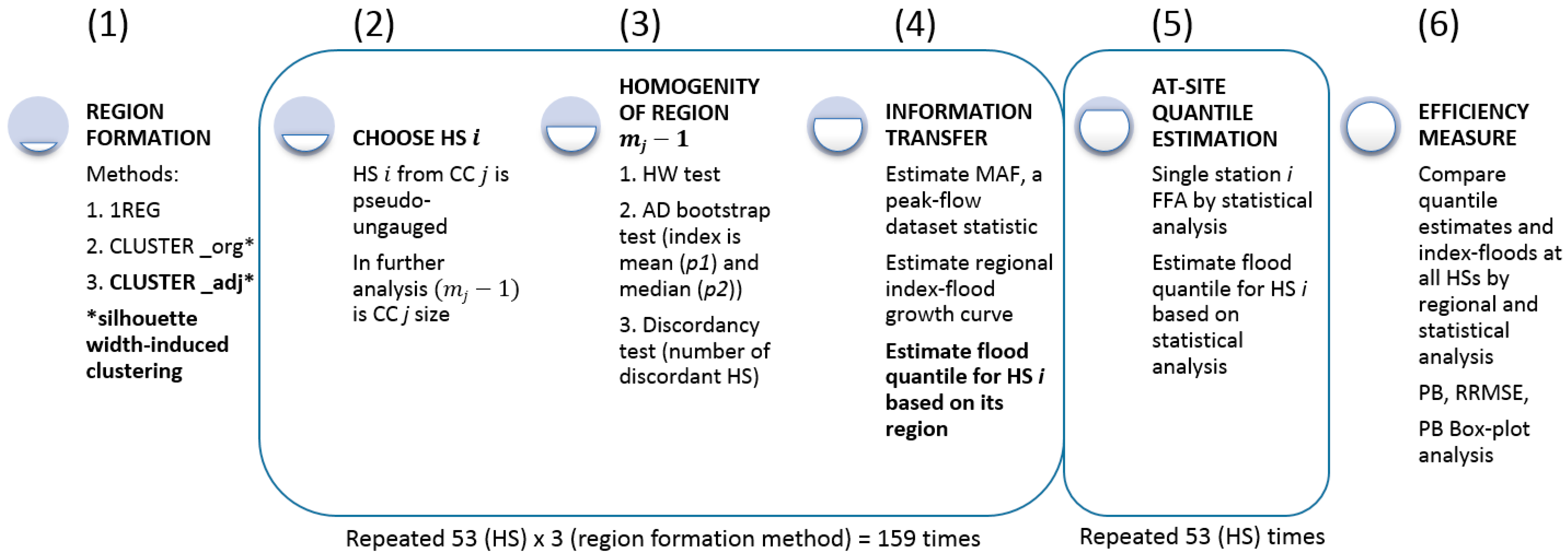
The research process consists of four phases, as shown in Figure 2 as a computational workflow divided into 6 steps. The initial phase is the formation of flood estimation regions (Figure 2, column 1), the second phase is flood quantile estimation in pseudo-ungauged catchments (Figure 2, columns 2–4), the third phase is estimation of ‘true’ flood quantiles by FFA, and the final phase is the comparison of regionally assessed flood quantiles and true ones.

One subjective method and two objective methods are used to form the regions. The subjective method implies that all stations form one region (label 1REG), while in the objective methods, regions are formed by the cluster analysis (label CLUSTER). The results of cluster analysis are the regions CLUSTER_org (i.e., original) and CLUSTER_adj (i.e., adjusted). The difference between the two regions (CCs) is in the adjustments made to CLUSTER_adj from CLUSTER_org to achieve positive silhouette widths of all objects (HSs) in CCs (Figure 2, column 1).

The regional analysis starts with the formation of regions where the 53 HSs are distributed among clusters according to similarity. Then, one HS is left out (pseudo-ungauged catchment), and the homogeneity of its region (CC) is tested using the Hosking–Wallis (HW) test, Anderson–Darling (AD) bootstrap test, and identification of discordant stations. In such a region, both mean annual flood (MAF) and a regional growth curve are estimated (Figure 2, columns 2–4). The result is appraised with respect to flood quantile at studied HSs estimated by FFA (Figure 2, column 5). The procedure is repeated for each HS and the three regionalization methods. The regionalization methods are generally evaluated through percent bias (PB) and regional root mean square error (RRMSE) (Figure 2, column 6).

2.2.1. Formation of the Regions

The subjective approach to the formation of regions leads to one region comprising all HSs (1REG). A selected objective approach is the application of one of the clustering methods, leading to the formation of two sets of regions (CLUSTER).

In the cluster analysis, catchments are allocated to regions using a hierarchical agglomerative approach that classifies objects (catchments) according to morphological similarities. The morphological attributes should not exhibit significant correlation to avoid giving too much importance to individual attributes [43]. At the beginning of hierarchical clustering, each HS forms an object (cluster) for itself, and through a clustering algorithm, merging is performed at each level (height) until the clusters become one region. Ward’s algorithm is applied here, known for its advantage in the formation of compact regions [18,44].

The silhouette width is used for the selection of the number of centers. It is calculated as the ratio of the average distance of the object i from the others falling into the same center j and the maximum distance d from the objects of other centers:

$$s_i^j=\frac{b_i^j-a_i^j}{\max \left(a_i^j,b_i^j\right)}$$

(1)

where $s_i^j$ is the silhouette width of the object $i$ from the cluster (center) $j$, $a_i^j$ is the average distance between $i$-th vector in cluster $C_j$ and other vectors in the same cluster, and $b_i^j$ is the minimum average distance between $i$-th vector in cluster $C_j$ and other vectors in the remaining clusters $C_k$ (k = 1, …, K, k ≠ j):

$$a_i^j=\frac{1}{m_j-1}\sum _{\begin{array}{c}k=1\\ k\ne i\end{array}}^{m_j}d\left(X_i^j,X_k^j\right), i=1,\dots ,m_j$$

(2)

$$b_i^j=\underset{\begin{array}{c}n=1,\dots ,K\\ n\ne j\end{array}}{\min }\left\{\frac{1}{m_n}\sum _{\begin{array}{c}k=1\\ k\ne i\end{array}}^{m_n}d\left(X_i^j,X_k^j\right)\right\}, i=1,\dots ,m_j$$

(3)

where $d\left(X_i^j,X_k^j\right)$ is the distance between objects $X_i$ and $X_k$, $m_j$ is the number of objects in cluster $C_j$, $m_n$ is the number of objects in remaining clusters $C_k$, and $K$ is the number of cluster centers.

The silhouette width range is [−1, 1]. The closer the silhouette width is to 1, the more compact the cluster, and the object is assigned to an adequate center.

The selection of a number of centers is performed by maximizing the mean silhouette width (MSW). The label for this clustering method is _org (original), therefore regions are labelled CLUSTER_org.

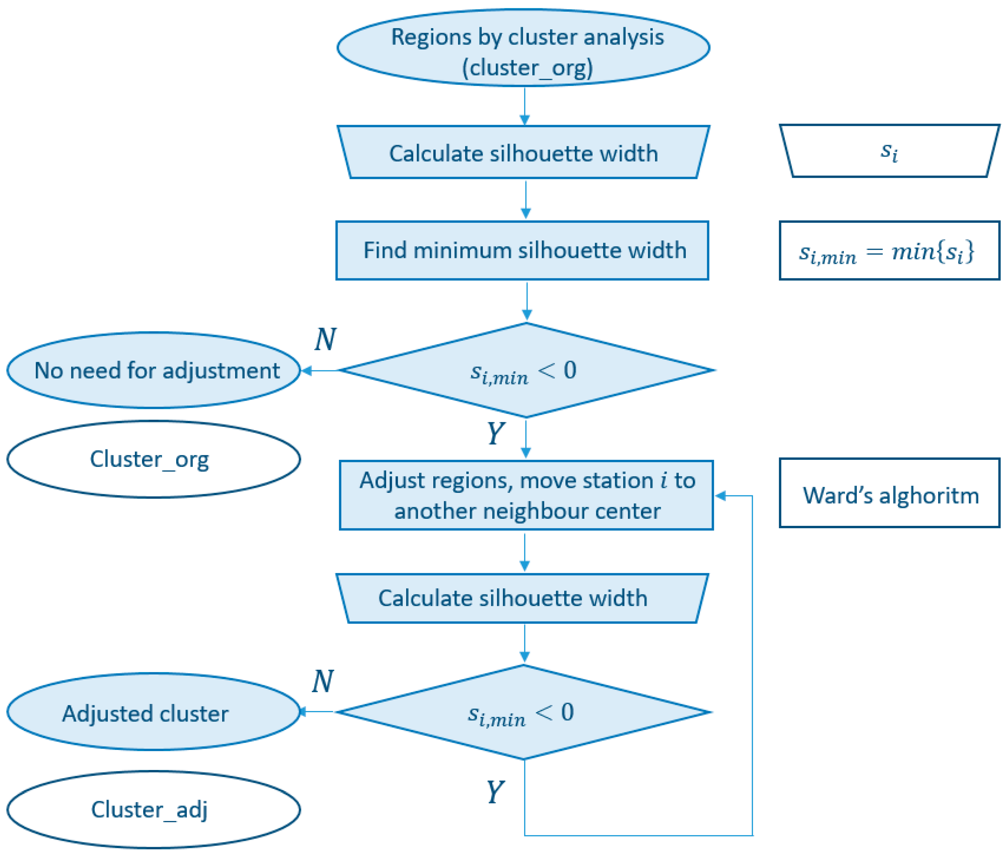
An issue in the _org clustering method is the presence of silhouette widths close to zero and negative. In the former case, it is inconclusive whether the object is in the adequate center. Negative silhouette width is used as an indicator of the wrong center, and the regions are adjusted accordingly to achieve positive silhouette widths (CLUSTER_adj).

The adjustment starts from the original regions CLUSTER_org and it is checked whether the smallest value of the silhouette width is negative. If so, the object is moved to the neighboring CC, and the silhouette widths are recalculated. The procedure stops when all silhouette widths are positive, as shown in the flow diagram in Figure 3.

2.2.2. Region Homogeneity Testing

The region homogeneity is tested for each regionalization method and HS. The pseudo-ungauged HS is left out from its region, and the homogeneity of the remaining m_j − 1 stations in the region is examined. Two tests were used: the parametric Hosking–Wallis (HW) test and the Anderson–Darling (AD) bootstrap test. Additionally, the number of discordant sites (HSs) is sought.

The HW test is based on the comparison of deviations (dispersion) of dimensionless moments with deviations in homogeneous regions. If the deviations are small enough, they are attributed to sampling error and the region is considered homogeneous.

The measures of dispersion are [17]

$$V={\left(\frac{\sum _{i=1}^{m_j-1}{n}_i{\left(t^{\left(i\right)}-t^R\right)}^2}{\sum _{i=1}^N{n}_i}\right)}^{\frac{1}{2}},$$

(4)

$$V_2=\frac{\sum _{i=1}^{m_j-1}{n}_i{\left\{{\left(t^{\left(i\right)}-t^R\right)}^2+{\left(t_3^{\left(i\right)}-t_3^R\right)}^2\right\}}^{1/2}}{\sum _{i=1}^N{n}_i},$$

(5)

$$V_3=\frac{\sum _{i=1}^{m_j-1}{n}_i{\left\{{\left(t_3^{\left(i\right)}-t_3^R\right)}^2+{\left(t_4^{\left(i\right)}-t_4^R\right)}^2\right\}}^{1/2}}{\sum _{i=1}^N{n}_i},$$

(6)

where t, t₃, and t₄ are dimensionless L-moments at HS (i) and region (R). Regional dimensionless moments are calculated as average by weighting local values by dataset size n_i:

$$t^R=LCv=\frac{\sum _{i=i}^{m_j-1}{n}_i{t}^{\left(i\right)}}{\sum _{i=1}^{m_j-1}{n}_i},$$

(7)

$$t_3^R=LCs=\frac{\sum _{i=i}^{m_j-1}{n}_i{t}_3^{\left(i\right)}}{\sum _{i=1}^{m_j-1}{n}_i},$$

(8)

$$t_4^R=LCk=\frac{\sum _{i=i}^{m_j-1}{n}_i{t}_3^{\left(i\right)}}{\sum _{i=1}^{m_j-1}{n}_i},$$

(9)

Following the procedure of Hoskings and Wallis [17], dispersion of each measure expected in homogeneous regions is obtained via 500 Monte Carlo simulations (N_sim = 500). The four-parameter kappa distribution is specified. Based on dispersion statistics (mean ${\mu }_V$ and standard deviation ${\sigma }_V$) H1, H2, and H3 measures are calculated as [17]

$$H1=\frac{\left(V-{\mu }_{V}1\right)}{{\sigma }_{V1}},H2=\frac{\left(V_2-{\mu }_{V2}\right)}{{\sigma }_{V2}},H3=\frac{\left(V_3-{\mu }_{V3}\right)}{{\sigma }_{V3}}$$

(10)

A region is considered ’acceptably homogeneous’ if H test statistics are less than 1 and ‘definitely heterogeneous’ for values greater than 2. The range between 1 and 2 is the ‘possibly homogeneous’ region. Even in extremely heterogeneous regions, H2 and H3 rarely reach values higher than 2 [19], so only H1 is used to check the homogeneity of the region.

In addition to the HW test, the AD bootstrap test was performed, recommended in cases of significant regional LCs values (greater than 0.23) [45]. The test is based on the comparison of local and regional empirical distribution functions as

$${\mathrm{\Theta }}_{AD}=\sum _{i=1}^k{n}_i{\int }_{\forall x}^{}\frac{{\left[\widehat{F_i}\left(x\right)-H_N\left(x\right)\right]}^2}{H_N\left(x\right)\left[1-H_N\left(x\right)\right]}d{H}_N\left(x\right).$$

(11)

where $\widehat{F_i}\left(x\right)$ is an empirical function of the i-th sample (HS) of length n_i, and $H_N\left(x\right)$ is a regional empirical function defined from sample size $N=n_1+\cdots +n_k$.

To avoid false conclusions about homogeneity, the nonparametric bootstrap procedure [45] is applied.

The third region homogeneity insight is obtained from the detection of discordant HSs. The discordant HS is the one far away from the centroid of the cloud of points in the dimensionless L-moments space.

The distance of each point is defined as [17]

$$D_i=\frac{1}{3}N{\left(u_i-\overline{u}\right)}^T{A}^{-1}\left(u_i-\overline{u}\right),$$

(12)

where $u_i$ is the vector of dimensionless moments at HS i $u_i=\left[t^{\left(i\right)},t_3^{\left(i\right)},t_4^{\left(i\right)}\right]$, $\overline{u}$ is the vector of unweighted individual vectors, and matrix A is defined as

$$A=\sum _{i=1}^N\left(u_i-\overline{u}\right){\left(u_i-\overline{u}\right)}^T.$$

(13)

The critical test values depend on the region size and range from 2.491 for 5 HSs to 3 for regions with more than 15 HSs [17].

2.2.3. Flood Information Transfer

The index-flood method is intended for regional flood frequency analysis [46,47]. This method combines data from several HSs to obtain one theoretical distribution function, i.e., regional growth curve, supposing an index (scaling factor) can be found at ungauged HS elsewhere or by some other method [17].

The mean annual flood (MAF) is selected as an index-flood statistic (index) here. For the pseudo-ungauged HS i, MAF is calculated by regression analysis, with one independent variable, a morphologic attribute:

$${MAF}_i=a·{ATTRIBUTEi}^b$$

(14)

Catchment area A, the average catchment elevation Havg, and the average catchment slope Iavg are considered as attributes.

Estimation of regression coefficients a and b in Equation (14) is performed using the least square method for 1REG and CLUSTER regions.

The regional growth curve is adopted based on the proximity of regional values on the L-moment plot (Section 3.3.2). The GEV distribution is selected for regional distribution with a regional growth curve.

2.2.4. At-Site Flood Quantile Estimation

The selection of GEV distribution for at-site flood quantile estimation is based on the research results for the same study region (HSs) [34], where five distribution functions in FFA are tested: Log-normal (LN), Gumbel (GUMB), exponential (EXP), Pearson 3 (P3), Log Pearson 3 (LP3), Generalized Extreme Values (GEV), and General Logistic (GLO). The Probability Plot Correlation Coefficient (PPCC) test showed that the GEV, LP3, and GLO functions are overall best ranked among the tested distribution functions [34].

GEV has been confirmed as the best distribution function in a large number of European basins [48,49] and beyond [50,51]. As a positive feature, the consistent estimation of the confidence interval is found [52], as well as minor sensitivity of the right distribution tail to low outliers, which is of considerable practical importance in flood analysis [53].

2.2.5. Efficiency of the Regionalization Methods

The efficiency of the applied regionalization methods for flood quantile assessment is analyzed for variables estimated in the regionalization procedure: MAF, 100-year flood quantiles, and the ratio of MAF to 100-year flood quantiles (

Table 1. Meaning of the variables in the regionalization efficiency analysis.

Label\Variable	MAF	Q100	q100
$x_{REG}$	${MAF}_{reg}$	${Q100}_{reg}$	$\frac{{Q100}_{reg}}{{MAF}_{reg}}$
$x_{obs}$	${MAF}_{at-site}$	${Q100}_{{at-site}_{}}$	$\frac{{Q100}_{at-site}}{{MAF}_{at-site}}$

). The flood quantile Q100 is selected for the efficiency analysis because an average peak flow dataset size in HSs of N = 51 years corresponds to the recommendation for the reliability of quantile estimation related to a return period of T < 2N–3N [13,54].

Two efficiency measures are calculated: relative bias and regional root mean square error (Equations (15) and (16)). Variables estimated in the at-site FFA are considered ‘observed’ in the efficiency assessment, as shown in Table 1.

Relative bias of regionalized (modelled) values:

$$PE=\frac{\left(x_{REG}-x_{obs}\right)}{x_{obs}}100$$

(15)

Regional Root Mean Square Error (RMSE):

$$RMSE=\sqrt{\frac{1}{N}\sum _{i=1}^N\frac{{\left(x_{REG}-x_{obs}\right)}^2}{x_{obs}}},$$

(16)

3. Results

3.1. Formation of Regions

Regions were formed in two ways: subjectively (a region comprising all HSs, label 1REG) and by hierarchal cluster analysis applying Ward’s algorithm (label CLUSTER), where the selection of similarity attributes was performed according to correlation significance (p-value) calculated for Pearson R² and Spearman ρ (rho) coefficients (

Table 2. The correlation indicators of morphologic attributes in the study region (53 HSs): the Pearson R² (upper table part below the diagonal) and its significance—p-values (upper table part above the diagonal); Spearman ρ coefficient (lower table part below the diagonal) and its significance—p-values (lower table part above the diagonal).

R2\p Value	A	Iavg	Havg
A	-	0.5457	0.8055
Iavg	−0.08	-	0.0000 *
Havg	−0.03	0.54	-
ρ\p value	A	Iavg	Havg
A	-	0.2716	0.7279
Iavg	−0.15	-	0.0000 *
Havg	0.05	0.53	-

* Significant correlation.

). According to the results, basin area ($A$) and mean catchment elevation ($Havg$) are selected.

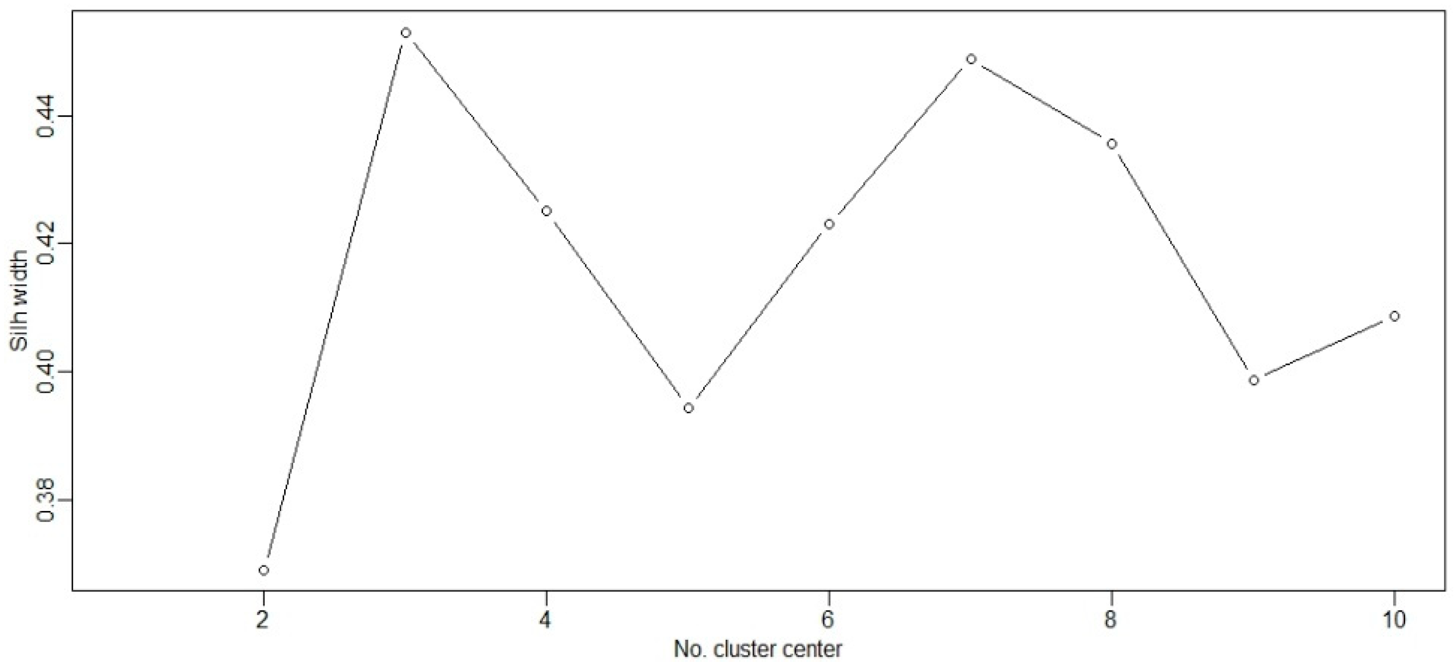
The merging flow of HSs in the objective regionalization method is shown by a dendrogram, providing the opportunity to designate regions for any number of CCs (Figure 4). The selection of a number of centers was performed by maximizing the mean silhouette width (MSW) (Figure 5). However, this cannot be a sole criterion because it is recommended that the number of objects in clusters is between 5 and 20 in hydrological research [24]. A compromise is found with 6 CCs, with 15, 5, 5, 5, 7, and 16 HSs comprising region CLUSTER_org (Figure 4). The locations of catchments according to CCs are shown in Figure A2 and Figure A3.

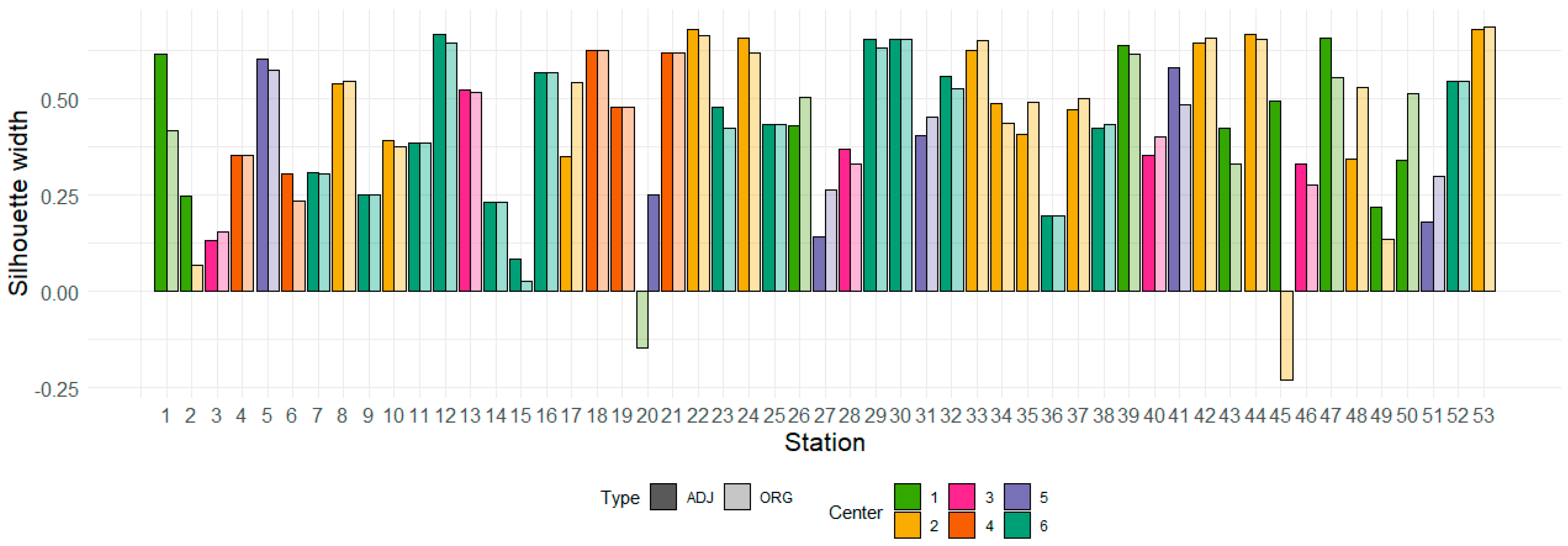
In the CLUSTER_org, HS20 and HS45 have a negative silhouette width (Figure 6). It took four iterations from CLUSTER_org to obtain CLUSTER_adj by the positive silhouette-width-induced clustering. The silhouette widths calculated in the original and adjusted procedures for each HS are shown in Figure 6. Three HSs moved from CC2 to CC1 (HS 2, 45, and 49), and HS 20 moved from CC1 to CC5. The difference in silhouette widths at some stations is notable, e.g., HS 1, HS 15, and HS 41, for better but HS 27, HS 50, and HS 51 for worse.

3.2. Region Homogeneity

Regional homogeneity was tested according to the H1 measure (HW test) and p1 and p2 values (AD bootstrap test adopting mean and median as index values, respectively). The conclusion was derived based on 500 simulations conducted in R using the {nsRFA} library. The consistency of HW and AD bootstrap tests is shown by the number of regions that matched the test conclusion (both accepted or both rejected homogeneity null hypothesis at the 5% significance level) and the number of regions where this was not the case (inconsistent results) (

Table 3. Region homogeneity testing results according to the HW test (H1) and AD bootstrap test (p1 and p2) shown as the number of HSs where results are realized in all regions/regions of cluster centers 1, 2, and 5.

Testing Results	_org		_adj
	p1 and p2	p1 and H1	p1 and p2	p1 and H1
Both positive (homogeneous region)	11/5	14/6	21/15	22/14
Both negative (heterogeneous region)	20/9	22/11	22/11	21/10
Inconsistent	22/14	17/11	10/2	10/4

). Homogeneity was tested for each pseudo-ungauged HS (its region). A comparison of homogeneity testing results in Table 3 shows that _adj clustering provided more consistent results, e.g., the number of HSs with inconsistent conclusion in _adj is 10/2 (p1 and p2), i.e., 10/4 (p1 and H1) compared to 22/14 and 17/11 in _org clustering.

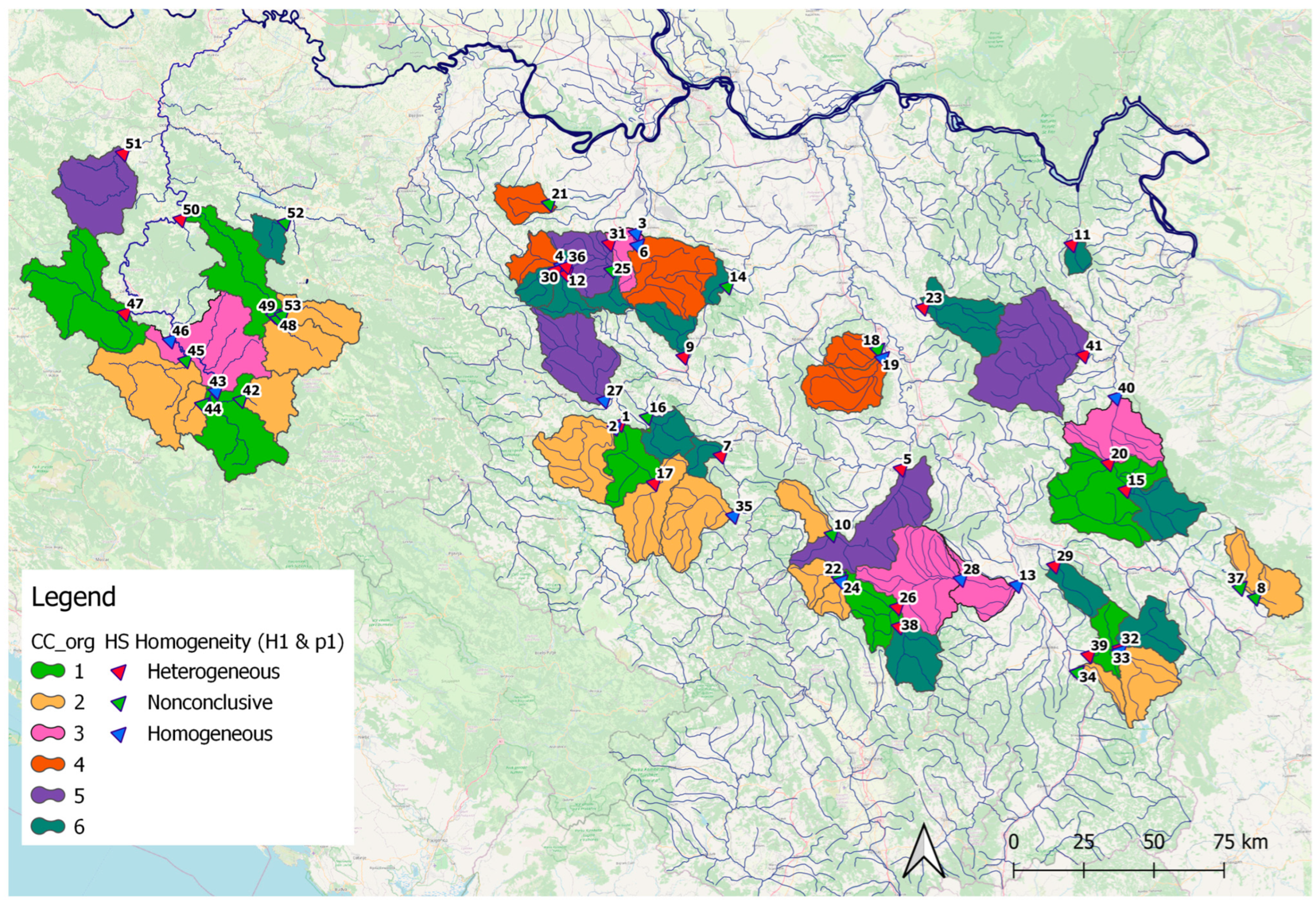
Figure 7 shows an individual homogeneity class at each HS based on the results consolidated in

Table 4. Relative Bias (%) of MAF estimation by regression for the three regionalization methods. The main components of boxplot diagrams. The best results are bolded.

Relative Bias	1REG	Cluster_Org	Cluster_Adj
Min	−58.93	−70.31	−70.31
1st quartile	−24.09	−27.33	26.67
3rd quartile	36.68	18.14	25.21
Max	128.2	165.4	133.5
IQR	60.77	45.47	51.88
Median	1.95	5.83	1.42
Mean	6.95	7.96	6.50
RRMSE	39.9	49.1	43.5

(p1 and H1) as well as the presence of a discordant station when that HS is left out (pseudo-ungauged). From Figure 7, it can be seen that twelve HSs should further produce reliable results in both _org and _adj cluster centers because their estimations will come from definitely homogeneous regions, free from discordant stations. These HSs are HS 43 (CC1), HS 24 and HS 35 (CC2), HS 3, 13, 28, 40, and 46 (CC3), HS 4, 6, and 19 (CC4), and HS 27 (CC5).

3.3. Flood Information Transfer

3.3.1. Mean Annual Flood (MAF)

The selection of an appropriate attribute (independent variable) in the regression equation (14) for MAF prediction is based on the relative bias of MAF estimation via attributes A, Iavg, and Havg for region 1REG. The best agreement of MAF (the smallest relative bias range) is achieved for catchment area (A) with the highest values of R² (close to 0.8). Still, a relative bias at individual HSs ranges from approximately −60% to 130% in respect of MAF at-site.

In Figure 8, the regression plots and 0.95 confidence intervals for MAF prediction in all CCs are shown, with catchment area as the predictor variable in the regions pooled by the _org and _adj approach. The figure shows three separate sets of regression lines, according to the differences in CCs in these two clustering approaches, taking into account $m_j$ stations.

In the course of MAF estimation for a pseudo-ungauged HS, the regression equation in its CC is redefined, i.e., regression coefficients are recalculated from the remaining m_j − 1 HSs in the CC. When analyzing pseudo-ungauged HSs from CC5 and partly CC3, the regression line slope becomes illogical, resulting in a MAF decrease with a catchment area increase. CC5 consists of HSs with catchment areas ranging from 630 km² to over 1100 km², with karst shares from 0% to 45%. Neglecting HS 46 in the CC3 also yields a negative value of the exponent b, leading to the largest MAF underestimation of all HSs. This is further discussed in Section 4.

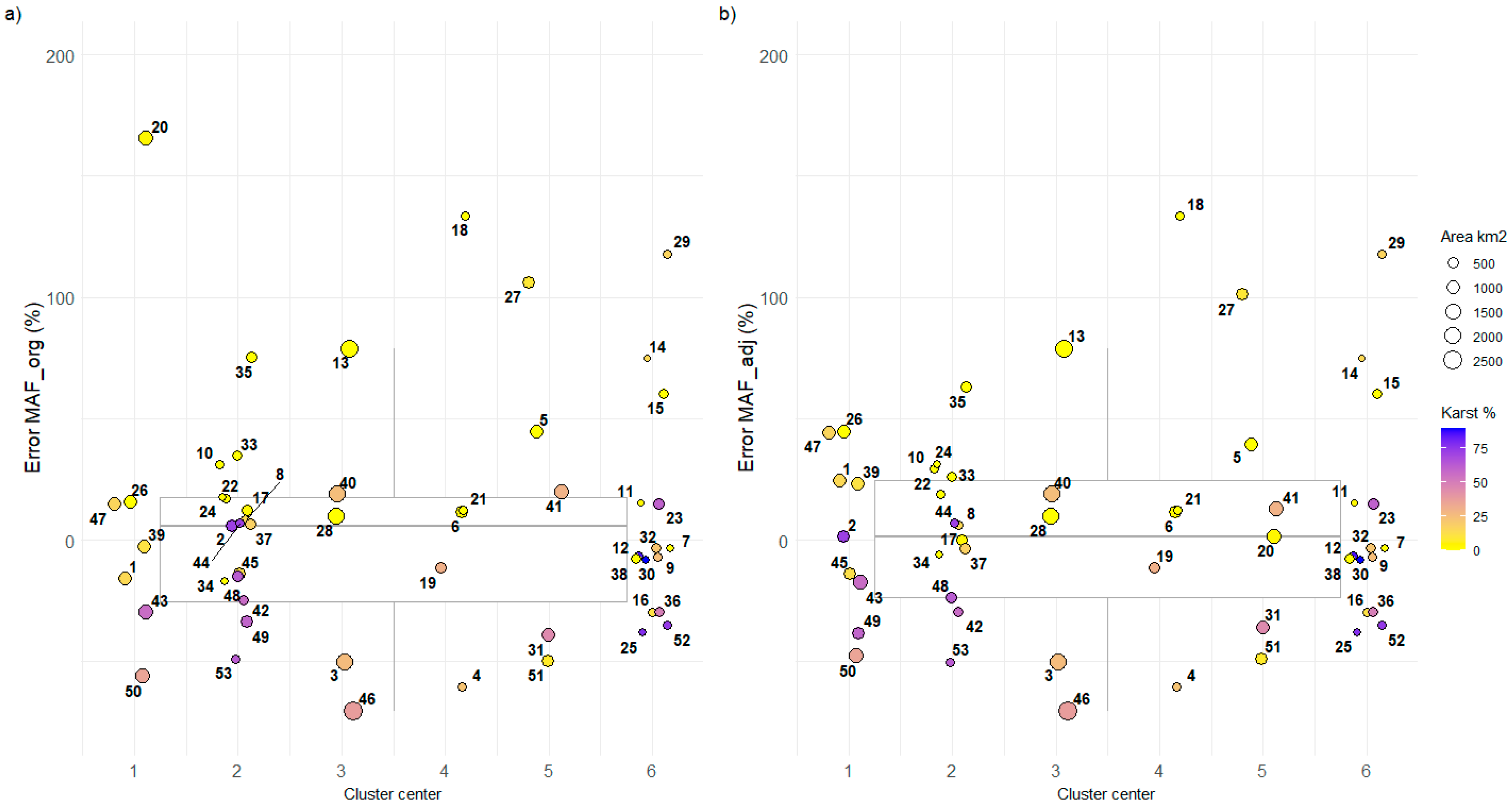
A significant MAF relative bias is generally found in HSs with catchment area extremes (min/max) in their CCs but also in the CCs comprising similar catchment area HSs but with significantly different karst shares. The HSs with min/max catchment area within the CC gave good MAF estimation agreement if the CC comprises HSs with similar catchment areas and karst shares. However, there are HSs of similar catchment area(s) and karst share that behave differently. In both _org and _adj CCs, MAF is generally underestimated in catchments with a high karst share.

Table 4 shows the consolidated efficiency measures of MAF prediction obtained for all HSs and shown per the regionalization method with the best values bolded; these are shown as components of boxplot diagrams in Figure 9.

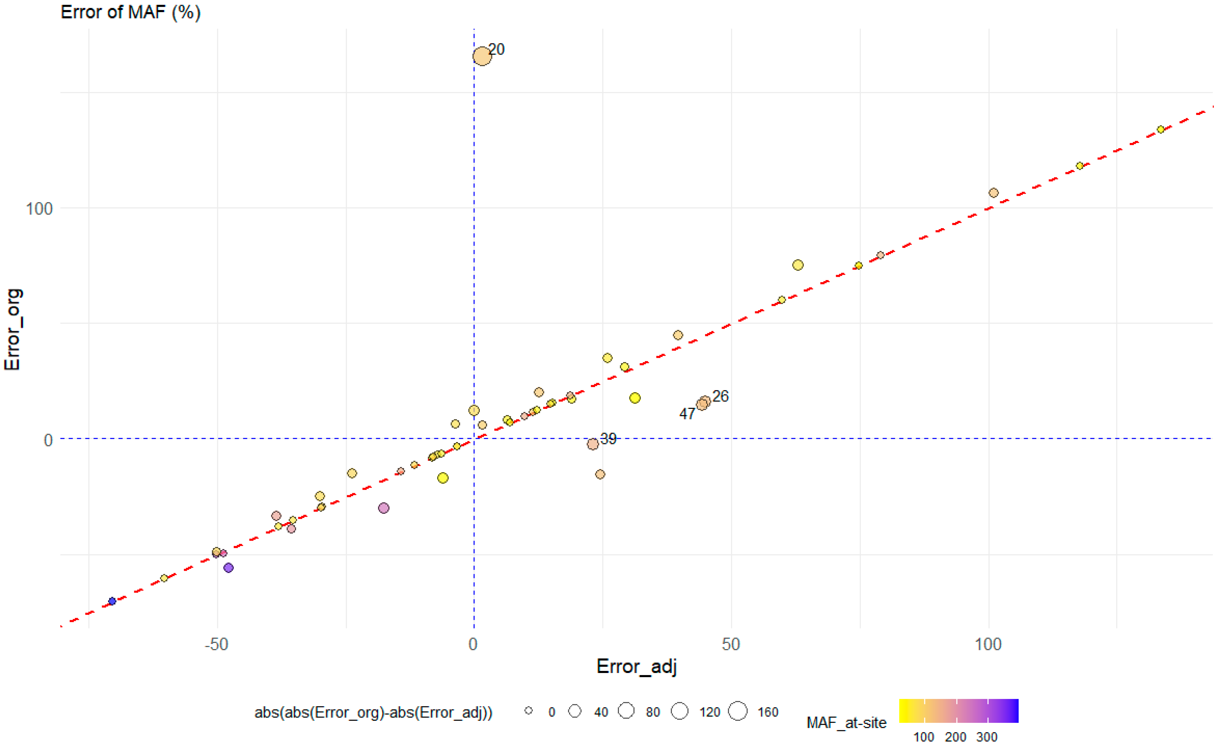
The relative bias in MAF estimates by the regression equations at all HSs in the _org and _adj clusters is shown in Figure 10. The dashed red line represents the location of a supposed equal MAF relative bias obtained for an HS in its _org and _adj cluster center.

The overall impression from Figure 10 is that there are more HSs with better individual results in MAF estimation from _adj clusters (14 HSs) compared to _org clusters (10 HSs), while the remaining 29 HSs (_org = _adj on the red dashed diagonal) lead to an equal MAF relative bias. The most underestimated MAFs (−70% to −50%) in both _org and _adj clusters are found for the HSs with high at-site MAF.

3.3.2. Regional Growth Curves

The selection of the regional growth curve distribution function is based on the L-moment plot, i.e., on the proximity of regional values for t₃ and t₄ parameters to the line representing a theoretical function. Regional parameter values calculated from $m_j$ stations ($m_j$ = 53 in 1REG) and for all CCs in the CLUSTER method are shown in Figure 11. For most regions, point (t₃, t₄) lies by the GEV line. Therefore, the GEV function is adopted for all regions.

Regional growth curves are constructed for all regions (e.g., dashed line for region 3 in Figure 12). Each pseudo-ungauged HS has its own regional growth curve because it is estimated from the m_j − 1 HS data.

The flood information transfer is completed by MAF estimation in an ungauged HS according to its catchment area and the construction of a regional growth curve for its region. Then, for a desired return period T, QT/MAF is known from the regional growth curve, the ratio is multiplied by MAF, and the flood quantile QT is estimated.

3.4. Regional 100-Year Flood Quantile Estimates

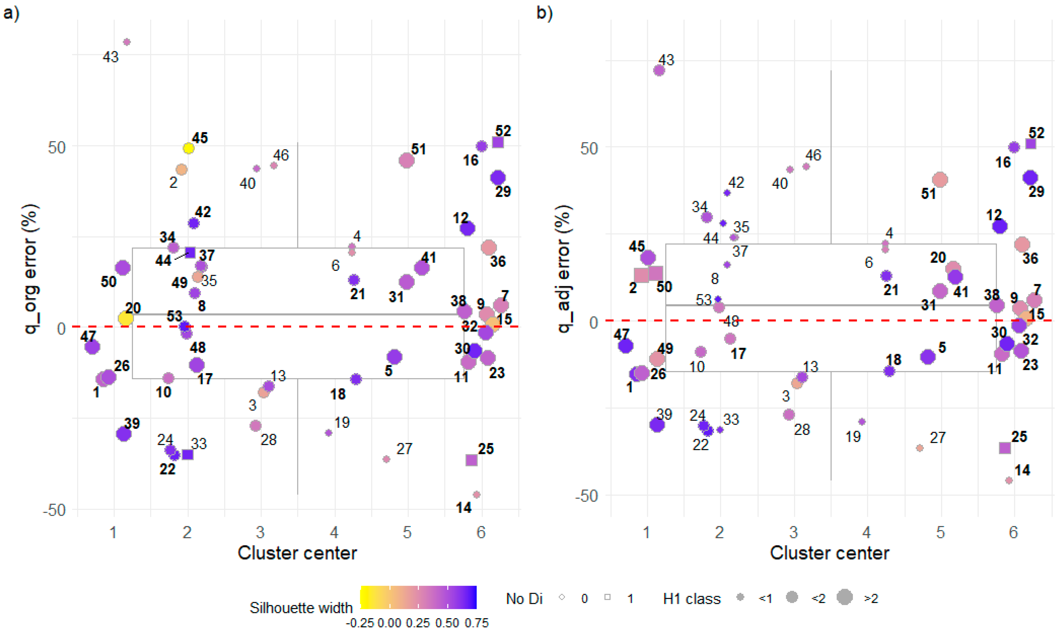
The flood quantile estimates are analyzed for the return period T of 100 years. The results are presented for the ratio q100 = Q100/MAF obtained from the regional growth curves and for flood quantile Q100. The relative bias (%) of q100 and Q100 estimates with respect to at-site values is shown in Figure 13 and Figure 14, respectively, as boxplots. The HSs are located in their corresponding regions/CCs in _org and _adj regionalization, with markers depicting silhouette width and region homogeneity measure H1 (HW test).

The range of relative bias in the q100 estimates in Figure 13 is smaller in homogeneous and possibly homogeneous regions (CC3, CC4, and CC2 for _adj), compared to the range in definitively heterogeneous regions (CC1, CC5, CC6, and CC2 for _org). The most obvious range shrinkage is in CC2 in _adj clustering (Figure 13b) compared to _org clustering (Figure 13a). A situation in Figure 14 depicting Q100 estimates relative to bias shows that after adjustment, definitely heterogeneous regions of CC1 and CC5 have a smaller range/more compact Q100 results compared to other CCs (Figure 14a compared to Figure 14b).

In Q100 estimation, apart from q100, MAF estimation plays an important role. The overall efficiency results of silhouette width _org and _adj clustering achieved for q100 and Q100 estimates is given in

Table 5. Relative Bias (%) in regional 100-year flood quantile estimation for silhouette-width-induced clustering. Regional RMSE (RRMSE) is also shown. The best results are bolded.

	Relative Bias	1REG	Cluster_Org	Cluster_Adj
q100	Min	−54.37	−46.08	−46.08
	1st quartile	−16.13	−14.15	−14.72
	3rd quartile	23.6	21.98	23.09
	Max	111.91	78.35	71.89
	IQR	39.72	36.14	37.82
	Median	3.44	3.43	4.26
	Mean	6.75	5.45	4.96
	RRMSE	31.35	27.98	26.61
Q100	Min	−71.18	−60.74	−60.74
	1st quartile	−26.17	−23.24	−16.67
	3rd quartile	34.91	28.80	25.77
	Max	147.91	207.35	207.35
	IQR	61.08	52.04	42.45
	Median	−0.31	0.58	2.43
	Mean	11.26	9.63	7.74
	RRMSE	47.33	51.80	45.60

. Almost all considered measures are slightly better in _adj compared to _org clustering and are shown in bold.

At the individual HS level, there are HSs with significant silhouette width but poor Q100 estimates, e.g., HS 29 in CC6 and HS 18 in CC4.

4. Discussion

There are two approaches in the comparison of regionalization methods: the first approach ends with the definition of homogeneous regions, and the second approach continues through information transfer down to the results of regionally assessed values [55]. The second approach is a performance-based assessment, conducted here with a focus on the silhouette-width-induced clustering outcome in flood quantile estimates. This approach has its known drawbacks due to uncertainty accumulation as the assessment advances (e.g., [17,55]).

Clustering based on silhouette width has so far been performed in other disciplines on large data samples, resulting in fewer CCs/regions compared to the number used here for flood quantile estimation [40].

Marková et al. [56] found 3 regions for flood seasonality in 556 Slovak and Austrian catchments where the optimal number of clusters was found according to the mean silhouette width (MSW). It was not shown whether these regions are homogenous.

The choice between an optimal number of regions here is also made according to maximized MSW, between possibly 3 and 7 (Figure 5), while trying to achieve the recommended number of elements, i.e., HSs in a region for hydrological applications [17,23].

Table 6. Mean silhouette width (MSW) and number of HSs (m_j) within each cluster center (CC).

	CC	1	2	3	4	5	6
MSW	_org	0.398	0.458	0.336	0.462	0.415	0.417
	_adj	0.452	0.534	0.341	0.476	0.360	0.429
mj	_org	7	16	5	5	5	15
	_adj	9	13			6

shows realized MSWs in six regions and their size.

According to the Rousseeuw’s MSW range [38], region/CC2_adj has a strong clustering structure (0.51 < MSW < 0.70), while the rest of the regions have weak clustering structures (0.26 < MSW < 0.50). The sizes of the individual regions are between the recommended 5 and 20.

The region size plays an important role in homogeneity determination [17]. Small regions may lead to false homogeneity conclusions, large regions are rarely homogenous, and comparison among regions with different sizes is complicated due to the ‘regional homogeneity’ concept, which is different from the heterogeneity concept considered in other fields [55]. Therefore, Requena et al. [55] proposed using the Gini index (GI) as a regional homogeneity (heterogeneity) measure that overpowers HW and AD tests in many aspects. In further research, GI will be used because the results obtained for pseudo-ungauged HSs here have shown that good Q100 estimation results originate from both homogeneous and heterogeneous regions. In the _adj CCs, the conclusions of the HW and AD bootstrap tests are more consistent compared to the _org CCs (Table 3), and the efficiency measures of MAF (Table 5), q100, and Q100 (Table 6) are overall better, although some values are significantly underestimated or overestimated.

When strictly observing results obtained from the homogenous region CC2_adj, which also has the best MSW among all CCs and a balanced size, the range of percent bias in Q100 is −50% to 40%, with one high outlier of 100%. The resulting bias range in q100 is from—24% to 30%. Such results point to the poor performance of the catchment area as an attribute used in the flood transfer model.

A single regression was used as a transfer model, with the catchment area as an independent variable. Despite significant values of R², large percent biases in MAF were observed in the subsequent jackknife procedure. It is assumed that this simple regression model is not adequate and that new variables should be introduced. The selection of new variables is not straightforward [57,58]. In a recent performance-based regionalization study for Ethiopia [59], 27 catchment attributes were considered: 9 morphologic and location, 5 soil, 12 land use, and mean annual rainfall. In the three homogeneous regions out of the four defined, MAF regression equations were developed using a total of six attributes: three morphologic, two land use, and one soil. Per each region, the MAF relative errors were 51%, 4%, and 17%. The flood quantile comparison was not shown. De Michele and Rosso [60] have shown a multi-level approach to flood frequency regionalization based on physical and statistical criteria/attributes. Flood, streamflow, and rainfall seasonality were studied and two indices were used to cluster catchments with the same flood production mechanism. In the area of Northwestern Italy, similar to the one studied here, 80 HSs were used, and 4 regions were defined according to seasonality analysis. It appears that precipitation and flood characteristics are unavoidable candidates for further attribute inclusion in regionalization. Additionally, in FFA, it is assumed that the upper limit of the Cs of flood flow is limited by the Cs of precipitation [61]. This means that not only can precipitation data be used as an attribute, but they could explain suspicious values of regionally assessed flood quantiles as well. Sometimes, in such cases, the value of the distribution parameters is limited to acceptable values [62].

The geological structure of the 53 catchments considered here is characterized by a wide range of karst content [34]. It is known that karst potentially reduces or amplifies flood peaks and influences the catchment boundary due to the complex conditions for surface and groundwater flow [63,64]. A karst share influence on MAF prediction is implicitly shown in Figure 9, where it may be observed that MAF in catchments with high karst share (>50%) is generally underestimated.

Apart from catchment attribute selection in MAF regression, the region size influences the reliability of regression coefficient estimation. It is shown here that small regions with five HSs may lead to ill-posed regression lines, such as in CC5 (Figure 8). Mc Cuen [65] suggested four times more data than the number of parameters for reliable correlation estimation. In this regard, a simple regression model with two parameters requires eight data points (HSs), plus one for the (pseudo-) ungauged HS, meaning that nine HSs is the minimum size of a region. From this perspective, CC_adj 1, 2, and 6 and CC_org 2 have reliable MAF regression equations.

In the regional flood growth curve estimations, the GEV distribution function is used for all regions. According to the L-moment ratio plots (Figure 11), for three CCs (_org 5, _adj 5, and _adj 3) other functions fit better but the relative biases in q100 estimates are similar to other CCs (Figure 13). The adoption of different regional distribution functions in regions has been performed by other researchers (e.g., [59]), and this may contribute to result improvement in future research. Due to input data issues (e.g., data gaps), the use of LP3 with the expected moments algorithm (EMA) should be reconsidered [11]. Overall better Q100 estimates were achieved in previous research [33] conducted using the Hydrologic Engineering Center’s Statistical Software Package (HEC-SSP) where EMA is installed. In addition to the 53 HSs here, more HSs were included, and a study area comprising 74 HSs was delineated in the three regions. The study period was 1961–1990.

The silhouette width of an individual HS has been shown as a good indicator of belonging to the wrong region but not as an indication of q100 or Q100 estimate quality in the circumstances presented here. The silhouette widths in HS 16 and HS 52 are among those showing a high clustering structure (>0.50). When these HSs are considered pseudo-ungauged in the jackknife procedure, the region is homogeneous (Figure 7), but their q100 estimates are among the most overestimated (~50%) (Figure 13). The percent biases in q100 or Q100 estimates in the region of CC_adj 2, holding most of the highest achieved silhouette widths among HSs, are slightly less spread compared to other CCs (Figure 13 and Figure 14). Still, the HSs with the highest silhouette widths are not those with the best q100 or Q100 estimates.

5. Conclusions

This study investigated the potential of silhouette-width-induced clustering according to catchment morphology similarity on the improvement of regionally based flood quantile estimates in 53 catchments situated in Bosnia and Herzegovina and Serbia. The ten HSs from Bosnia and Herzegovina are characterized by flood peak dataset gaps and the presence of karst, which are among the main issues in flood quantile estimation in practice. The HSs from Serbia were added for flood information improvement in the catchments from Bosnia and Herzegovina. The flood information transfer was performed for all catchments (HSs) using the jackknife procedure, thus showing percent bias with respect to ‘true’ values at each computational step. Flood quantile estimation from both homogeneous and heterogeneous regions allowed for the comparison of the extent of bias even when the flood estimation conditions were not fully met. The following is concluded:

• The mean silhouette width of a cluster is an indicator of region composition quality: the higher mean silhouette width of a region means less uncertainty in region homogeneity. The regions should be adjusted to comprise HSs with positive individual silhouette widths. However, high individual silhouette widths cannot indicate good performance in flood quantile estimation.
• Balancing region size is important. Maximizing the mean silhouette width of a region yields a small number of regions with a large number of HSs. On the other hand, large regions tend to be heterogeneous. The minimum number of HSs in the region depends on the selected information transfer method. When the regression equation is established for the assessment of mean annual flood, the minimum number of HSs in a region should be nine if a simple regression with one variable is planned, and four more HSs should be added per regression coefficient/independent variable.
• Despite the high values of R², single regression with catchment area as an independent variable gives significant relative bias in MAF.
• Similarity based on morphological attributes alone tends to result in regions that provide unreliable flood quantile estimates, even if the region is homogeneous, most likely due to an absence of local climate-/flood-related attributes.
• Good flood estimation results at individual HSs are achieved from both homogeneous and heterogeneous regions and for those containing discordant HSs. In addition to or instead of HW and AD bootstrap tests, an additional regional homogeneity insight should be introduced in future work by, e.g., the Gini Index (GI), to increase certainty about the results obtained from homogeneous regions.
• The use of one distribution function (GEV) for all regions in the index-flood method does not seem to significantly influence flood quantile estimates in this study.

References

1. Młyński, D.; Wałęga, A.; Ozga-Zielinski, B.; Ciupak, M.; Petroselli, A. New approach for determining the quantiles of maximum annual flows in ungauged catchments using the EBA4SUB model. J. Hydrol. 2020, 589, 125198. [Google Scholar] [CrossRef]
2. Adnan, R.M.; Petroselli, A.; Heddam, S.; Santos, C.A.G.; Kisi, O. Comparison of different methodologies for rainfall–runoff modeling: Machine learning vs conceptual approach. Nat. Hazards 2021, 105, 2987–3011. [Google Scholar] [CrossRef]
3. Reliability of Flood Discharge Estimates. Available online: https://cdnsciencepub.com/doi/10.1139/l91-076 (accessed on 26 February 2023).
4. Guerrero, J.-L.; Westerberg, I.K.; Halldin, S.; Xu, C.-Y.; Lundin, L.-C. Temporal variability in stage–discharge relationships. J. Hydrol. 2012, 446–447, 90–102. [Google Scholar] [CrossRef]
5. Blöschl, G.; Hall, J.; Viglione, A.; Perdigão, R.A.P.; Parajka, J.; Merz, B.; Lun, D.; Arheimer, B.; Aronica, G.T.; Bilibashi, A.; et al. Changing climate both increases and decreases European river floods. Nature 2019, 573, 108–111. [Google Scholar] [CrossRef] [PubMed]
6. Tuel, A.; Eltahir, E.A.B. Why Is the Mediterranean a Climate Change Hot Spot? J. Clim. 2020, 33, 5829–5843. [Google Scholar] [CrossRef]
7. Kundzewicz, Z.W. Changes in Flood Risk in Europe; CRC Press: London, UK, 2019; ISBN 978-0-203-09809-7. [Google Scholar]
8. Chiaravalloti, F.; Caloiero, T.; Coscarelli, R. The Long-Term ERA5 Data Series for Trend Analysis of Rainfall in Italy. Hydrology 2022, 9, 18. [Google Scholar] [CrossRef]
9. Hundecha, Y.; Parajka, J.; Viglione, A. Assessment of past flood changes across Europe based on flood-generating processes. Hydrol. Sci. J. 2020, 65, 1830–1847. [Google Scholar] [CrossRef]
10. Zabolotnia, T.; Parajka, J.; Gorbachova, L.; Széles, B.; Blöschl, G.; Aksiuk, O.; Tong, R.; Komma, J. Fluctuations of Winter Floods in Small Austrian and Ukrainian Catchments. Hydrology 2022, 9, 38. [Google Scholar] [CrossRef]
11. England, J.F., Jr.; Cohn, T.A.; Faber, B.A.; Stedinger, J.R.; Thomas, W.O., Jr.; Veilleux, A.G.; Kiang, J.E.; Mason, R.R. Bulletin 17C Guidelines for Determining Flood Flow Frequency, Chapter 5 of Section B, Surface Water, Book 4, Hydrologic Analysis and Interpretation; U.S. Geological Survey: Reston, VA, USA, 2019.
12. СП 33-101-2003 Определение Оснoвных Расчетных Гидрoлoгических Характеристик. (Determination of Design Hydrological Performance). Available online: https://docs.cntd.ru/document/1200035578 (accessed on 23 February 2023).
13. German Association for Water Management, Sewage and Waste. DWA-M 552 Ermittlung von Hochwasserwahrscheinlichkeiten (Determination of Flood Probabilities); Lehmanns: Munich, Germany, 2012; ISBN 978-3-942964-25-8. [Google Scholar]
14. Merz, R.; Blöschl, G. Flood frequency hydrology: 1. Temporal, spatial, and causal expansion of information. Water Resour. Res. 2008, 44, W08432. [Google Scholar] [CrossRef] [Green Version]
15. Merz, R.; Blöschl, G. Flood frequency hydrology: 2. Combining data evidence. Water Resour. Res. 2008, 44. [Google Scholar] [CrossRef]
16. Blagojević, B.; Plavšić, J. A normalized regression based regional model for generating flows at ungauged basins. Water Sci. Technol. J. Int. Assoc. Water Pollut. Res. 2013, 68, 99–108. [Google Scholar] [CrossRef] [PubMed]
17. Hosking, J.R.M.; Wallis, J.R. Regional Frequency Analysis: An Approach Based on L-Moments; Cambridge University Press: Cambridge, UK, 1997; ISBN 978-0-521-43045-6. [Google Scholar] [CrossRef]
18. Rao, R. Srinivasan Regionalization of Watersheds an Approach Based on Cluster Analysis; Water Science and Technology Library; Springer: Dordrecht, The Netherlands, 2008; Volume 58, ISBN 978-1-4020-6851-5. [Google Scholar]
19. Gnanaprakkasam, S.; Ganapathy, G. Model-Based Clustering Approach for Regional Flood Frequency Analysis. Indian J. Ecol. 2019, 46, 493–504. [Google Scholar]
20. Burn, D.H. Evaluation of regional flood frequency analysis with a region of influence approach. Water Resour. Res. 1990, 26, 2257–2265. [Google Scholar] [CrossRef]
21. Zrinji, Z.; Burn, D.H. Flood frequency analysis for ungauged sites using a region of influence approach. J. Hydrol. 1994, 153, 1–21. [Google Scholar] [CrossRef]
22. Geological Survey (U.S.) (Ed.) Guidelines for Determining Flood Flow Frequency. Bulletin #17B of the Hydrology Subcommittee; Bulletin of the Hydrology Committee; Editorial Corrections March 1982; U.S. Department of the Interior, Geological Survey, Office of Water Data Coordination: Reston, VA, USA, 1982.
23. Blagojević, B. Razvoj Modela za Prostornu Interpolaciju Hidroloških Vremnskih Serija na Neizučenim Profilima. (Development of a Model for Spatial Interpolation of Hydrologic Time Series in Ungauged Catchments). Ph. D. Thesis, University of Niš, Faculty of Civil Engineering and Architecture, Niš, Serbia, 2011. [Google Scholar]
24. Cunnane, C. Methods and merits of regional flood frequency analysis. J. Hydrol. 1988, 100, 269–290. [Google Scholar] [CrossRef]
25. Mengistu, T.D.; Feyissa, T.A.; Chung, I.-M.; Chang, S.W.; Yesuf, M.B.; Alemayehu, E. Regional Flood Frequency Analysis for Sustainable Water Resources Management of Genale–Dawa River Basin, Ethiopia. Water 2022, 14, 637. [Google Scholar] [CrossRef]
26. Ouarda, T.B.M.J.; Cunderlik, J.M.; St-Hilaire, A.; Barbet, M.; Bruneau, P.; Bobée, B. Data-based comparison of seasonality-based regional flood frequency methods. J. Hydrol. 2006, 330, 329–339. [Google Scholar] [CrossRef]
27. Cunderlik, J.M.; Ouarda, T.B.M.J.; Bobée, B. On the objective identification of flood seasons. Water Resour. Res. 2004, 40, 1520. [Google Scholar] [CrossRef] [Green Version]
28. Gingras, D.; Adamowski, K. Homogeneous region delineation based on annual flood generation mechanisms. Hydrol. Sci. J. 1993, 38, 103–121. [Google Scholar] [CrossRef]
29. Komi, K.; Amisigo, B.A.; Diekkrüger, B.; Hountondji, F.C.C. Regional Flood Frequency Analysis in the Volta River Basin, West Africa. Hydrology 2016, 3, 5. [Google Scholar] [CrossRef] [Green Version]
30. Lecce, S.A. Spatial variations in the timing of annual floods in the southeastern United States. J. Hydrol. 2000, 235, 151–169. [Google Scholar] [CrossRef]
31. Parajka, J.; Kohnová, S.; Bálint, G.; Barbuc, M.; Borga, M.; Claps, P.; Cheval, S.; Dumitrescu, A.; Gaume, E.; Hlavčová, K.; et al. Seasonal characteristics of flood regimes across the Alpine–Carpathian range. J. Hydrol. 2010, 394, 78–89. [Google Scholar] [CrossRef]
32. Hrelja, H. Definiranje nekih elemenata hidrološkog režima metodom regionalizacije. Vodoprivreda 2005, 37, 21–34. [Google Scholar]
33. Mulaomerović-Šeta, A.; Blagojević, B.; Imširović, Š.; Nedić, B. Assessment of Regional Analyses Methods for Spatial Interpolation of Flood Quantiles in the Basins of Bosnia and Herzegovina and Serbia. In Proceedings of the Advanced Technologies, Systems, and Applications VI; Ademović, N., Mujčić, E., Akšamija, Z., Kevrić, J., Avdaković, S., Volić, I., Eds.; Springer International Publishing: Cham, Switzerland, 2022; pp. 430–456. [Google Scholar] [CrossRef]
34. Mulaomerović-Šeta, A. Primjena Regionalnih Analiza u Poboljšanju Ocjene Kvantila Velikih Voda. Ph.D. Thesis, University of Sarajevo, Faculty of Civil Engineering, Sarajevo, Bosnia and Herzegovina, 2022. [Google Scholar]
35. Mulaomerović-Šeta, A.; Blagojević, B.; Mihailović, V.; Lozančić, Ž. Flood Frequency Assessment in Data Poor Environment Case Study Maglaj-Poljice on the River Bosna. In Proceedings of the 4th International Conference on Multi-scale Computational Methods for Solids and Fluids, Sarajevo, Bosnia and Herzegovina, 18–20 September 2019; Ibrahimbegovic, A., Dolarevic, S., Džaferovic, E., Hrasnica, M., Bjelonja, I., Zlatar, M., Hanjalic-Sarajevo, K., Eds.; Faculty of Civil Engineering: Sarajevo, Bosnia and Herzegovina; pp. 39–42, ISBN 978-9958-638-57-2. [Google Scholar]
36. Radić, Z. Istorijska poplava na Gornjoj Drini 1896 godine, Zbornik radova sa 16. In Proceedings of the Naučnog Savetovanja Srpskog Društva za Hidraulička Istraživanja (SDHI) i Srpskog Društva za Hidrologiju (SDH), Donji Milanovac, Serbia, 22–23 October 2012; Ivetić, M., Kapor, R., Plavšić, J., Eds.; Univerzitet u Beogradu—Građevinski fakultet: Beograd, Srbija, 2012; pp. 605–618, ISBN 8675181590, 9788675181590. [Google Scholar]
37. Petroselli, A.; Mulaomerović-Šeta, A.; Lozančić, Ž. Comparison of methodologies for design peak discharge estimation in selected catchments of Bosnia and Herzegovina. J. Croat. Assoc. Civ. Eng. 2019, 71, 729–738. [Google Scholar]
38. Rousseeuw, P.J. Silhouettes: A graphical aid to the interpretation and validation of cluster analysis. J. Comput. Appl. Math. 1987, 20, 53–65. [Google Scholar] [CrossRef] [Green Version]
39. Goyal, M.; Gupta, V. Identification of Homogeneous Rainfall Regimes in Northeast Region of India using Fuzzy Cluster Analysis. Water Resour. Manag. 2014, 28, 4491–4511. [Google Scholar] [CrossRef]
40. Lengyel, A.; Botta-Dukát, Z. Silhouette width using generalized mean—A flexible method for assessing clustering efficiency. Ecol. Evol. 2019, 9, 13231–13243. [Google Scholar] [CrossRef] [Green Version]
41. Shutaywi, M.; Kachouie, N.N. Silhouette Analysis for Performance Evaluation in Machine Learning with Applications to Clustering. Entropy 2021, 23, 759. [Google Scholar] [CrossRef]
42. Imširović, Š. Regionalna Analiza Karakateristika Velikih Voda na Teritoriji Srbije i Bosne i Hercegovine u Periodu 1961–1990. Master’s Thesis, University of Sarajevo, Faculty of Civil Engineering, Sarajevo, Bosnia and Herzegovina, 2020. [Google Scholar]
43. Cluster Analysis Gets Complicated. TRC Market Research. Available online: https://trcmarketresearch.com/whitepaper/cluster-analysis-gets-complicated/ (accessed on 26 February 2023).
44. Bu, J.; Liu, W.; Pan, Z.; Ling, K. Comparative Study of Hydrochemical Classification Based on Different Hierarchical Cluster Analysis Methods. Int. J. Environ. Res. Public Health 2020, 17, 9515. [Google Scholar] [CrossRef]
45. Viglione, A.; Laio, F.; Claps, P. A comparison of homogeneity tests for regional frequency analysis. Water Resour. Res. 2007, 43, 1658. [Google Scholar] [CrossRef] [Green Version]
46. Dalrymple, T. Flood-Frequency Analyses, Manual of Hydrology: Part 3; U.S. Government Publishing Office: Washington, DC, USA, 1960. [CrossRef]
47. Aureli, F.; Mignosa, P.; Prost, F.; Dazzi, S. Hydrological and Hydraulic Flood Hazard Modeling in Poorly Gauged Catchments: An Analysis in Northern Italy. Hydrology 2021, 8, 149. [Google Scholar] [CrossRef]
48. Castellarin, A.; Kohnová, S.; Gaál, L.; Fleig, A.; Salinas, J.L.; Toumazis, A.; Kjeldsen, T.; Macdonald, N. Review of Applied-Statistical Methods for Flood-Frequency Analysis in Europe: WG2 of COST Action ES0901; (NERC) Centre for Ecology & Hydrology: Banchory, UK, 2012. [Google Scholar]
49. Progress in Modern Hydrology: Past, Present and Future, 1st ed.; Rodda, J.C.; Robinson, M. (Eds.) Wiley: New York, NY, USA, 2015; ISBN 978-1-119-07427-4. [Google Scholar] [CrossRef]
50. Haddad, K.; Rahman, A. Investigation on at-site flood frequency analysis in South-East Australia. Inst. Eng. Malays. 2008, 69, 59–64. [Google Scholar]
51. Vogel, R.M.; McMahon, T.A.; Chiew, F.H.S. Floodflow frequency model selection in Australia. J. Hydrol. 1993, 146, 421–449. [Google Scholar] [CrossRef]
52. Khan, Z.; Rahman, A.; Karim, F. An Assessment of Uncertainties in Flood Frequency Estimation Using Bootstrapping and Monte Carlo Simulation. Hydrology 2023, 10, 18. [Google Scholar] [CrossRef]
53. Blagojević, B.; Mihailović, V.; Plavšić, J. Statistička Analiza Velikih Voda Na Profilima Hidroloških Stanica: Potreba Za Promenom Pristupa|Časopis Vodoprivreda. Available online: https://www.vodoprivreda.net/statisticka-analiza-velikih-voda-na-profilima-hidroloskih-stanica-potreba-za-promenom-pristupa/ (accessed on 22 February 2023).
54. Vukmirović, V. Analiza Verovatnoće Pojave Hidroloških Veličina; Naučna Knjiga; Građevinski Fakultet: Beograd, Serbia, 1990; ISBN 978-86-23-41048-2. [Google Scholar]
55. Requena, A.I.; Chebana, F.; Ouarda, T.B.M.J. Heterogeneity measures in hydrological frequency analysis: Review and new developments. Hydrol. Earth Syst. Sci. 2017, 21, 1651–1668. [Google Scholar] [CrossRef] [Green Version]
56. Marková, R.; Kohnová, S.; Parajka, J. Detecting Similarity in Flood Seasonality of Slovak and Austrian Catchments. IOP Conf. Ser. Mater. Sci. Eng. 2019, 471, 022027. [Google Scholar] [CrossRef]
57. Merz, R.; Blöschl, G.; Humer, G. National flood discharge mapping in Austria. Nat. Hazards 2008, 46, 53–72. [Google Scholar] [CrossRef]
58. Merz, R.; Blöschl, G. Flood frequency regionalisation—Spatial proximity vs. catchment attributes. J. Hydrol. 2005, 302, 283–306. [Google Scholar] [CrossRef]
59. Kebebew, A.S.; Awass, A.A. Regionalization of catchments for flood frequency analysis for data scarce Rift Valley Lakes Basin, Ethiopia. J. Hydrol. Reg. Stud. 2022, 43, 101187. [Google Scholar] [CrossRef]
60. De Michele, C.; Rosso, R. A multi-level approach to flood frequency regionalisation. Hydrol. Earth Syst. Sci. 2002, 6, 185–194. [Google Scholar] [CrossRef]
61. McCuen, R.H.; Smith, E. Origin of Flood Skew. J. Hydrol. Eng. 2008, 13, 771–775. [Google Scholar] [CrossRef]
62. Ding, Q.; Arnaud, P. Taking Account of Seasonality in a Regional Flood Frequency Estimation Approach Based on Event Simulations. Water 2022, 14, 1376. [Google Scholar] [CrossRef]
63. Mance, D.; Radišić, M.; Lenac, D.; Rubinić, J. Hydrological Behavior of Karst Systems Identified by Statistical Analyses of Stable Isotope Monitoring Results. Hydrology 2022, 9, 82. [Google Scholar] [CrossRef]
64. Sarker, S.K.; Fryar, A.E. Characterizing Hydrological Functioning of Three Large Karst Springs in the Salem Plateau, Missouri, USA. Hydrology 2022, 9, 96. [Google Scholar] [CrossRef]
65. McCuen, R.H. Statistical Methods for Engineers; Prentice-Hall: Englewood Cliffs, NJ, USA, 1985; ISBN 978-0-13-844903-2. [Google Scholar]
Figure 1. Study region and catchments (thick black boundary lines) of hydrological gauge stations (numbered).
Hydrology 10 00126 g001
Figure 2. Computation workflow.
Hydrology 10 00126 g002
Figure 3. The silhouette-width-induced clustering—an adjustment procedure of the region size to achieve positive silhouette widths.
Hydrology 10 00126 g003
Figure 4. Dendrogram based on Ward’s clustering algorithm, using morphologic attributes A and Havg from 53 HSs shown by their labels (numbers). Each CC is presented in different color.
Hydrology 10 00126 g004
Figure 5. The change in mean silhouette width for the number of CCs.
Hydrology 10 00126 g005
Figure 6. The silhouette widths of HSs designated to centers (regions) in _org and _adj clustering. The bar color shows the corresponding HS center, and the transparency shows the clustering method.
Hydrology 10 00126 g006
Figure 7. Homogeneity class of each HS according to HW and AD bootstrap tests obtained when the HS is left out (pseudo-ungauged) and when a discordant HS is found in such region with (mj − 1) HSs.
Hydrology 10 00126 g007
Figure 8. Regressions in the form MAF = aAb in loge scale, with 0.95 confidence intervals for silhouette-induced clustering: (a) centers 3, 4, and 6 (_org = _adj), (b) centers 1, 2, and 5 in _org, and (c) centers 1, 2, and 5 in _adj. Color is an indicator of the HS cluster center.
Hydrology 10 00126 g008
Figure 9. MAF prediction efficiency from regression equations in the CCs shown as relative bias (error) realized for each HS in (a) CC_org and (b) CC_adj. Marker size corresponds to the catchment area, and marker color corresponds to karst share.
Hydrology 10 00126 g009
Figure 10. Relative bias in MAF estimates obtained in _org and _adj regionalization. Marker color indicates MAF at-site (m3/s), and marker size shows the extent of the MAF difference (%) in the _org and _adj approaches.
Hydrology 10 00126 g010
Figure 11. Regional values for the LCs = t3 and LCk = t4 parameters, with regions pooled by 1REG (marker +) and by cluster analysis (marker o) in the _org (transparent) and _adj (nontransparent) approaches. All HSs in the CCs are considered.
Hydrology 10 00126 g011
Figure 12. The regional growth curve in region 3. Colored lines show curves for QT/MAF estimation at individual HS (based on mj − 1 HSs), and the dashed line is the growth curve in the considered region (mj HSs).
Hydrology 10 00126 g012
Figure 13. Relative bias (%) in q100 estimates in (a) _org CCs and (b) _adj CCs. The marker’s color indicates silhouette width, its size indicates whether the q100 is estimated from a homogeneous, possibly homogenous, or heterogenous region—H1 class (small, medium, and large marker, respectively), and a square marker shows that the HS is found to be discordant in its region. HS numbers are by the markers.
Hydrology 10 00126 g013
Figure 14. Relative bias (%) in Q100 estimates in (a) _org CCs and (b) _adj CCs. The marker’s color indicates silhouette width, its size indicates whether the Q100 is estimated from a homogeneous, possibly homogenous, or heterogenous region—H1 class (small, medium, and large marker, respectively), and a square marker shows that the HS is found to be discordant in its CC. HS numbers are by the markers.
Hydrology 10 00126 g014