Spatiotemporal Variability in Total Dissolved Solids and Total Suspended Solids along the Colorado River

Abstract

The Colorado River is a principal source of water for 40 million people and farmlands in seven states in the western US and the Republic of Mexico. The river has been under intense pressure from the effects of climate change and anthropogenic activities associated with population growth leading to elevated total dissolved solid (TDS) and total suspended solid (TSS) concentrations. Elevated TDS- and TSS-related issues in the basin have a direct negative impact on the water usage and the ecological health of aquatic organisms. This study, therefore, analyzed the spatiotemporal variability in the TDS and TSS concentrations along the river. Results from our analysis show that TDS concentration was significantly higher in the Upper Colorado River Basin while the Lower Colorado River Basin shows a generally high level of TSSs. We found that the activities in these two basins are distinctive and may be a factor in these variations. Results from the Kruskal–Wallis significance test show there are statistically significant differences in TDSs and TSSs from month to month, season to season, and year to year. These significant variations are largely due to seasonal rises in consumptive use, agriculture practices, snowmelts runoffs, and evaporate rates exacerbated by increased temperature in the summer months. The findings from this study will aid in understanding the river’s water quality, detecting the sources and hotspots of pollutions to the river, and guiding legislative actions. The knowledge obtained forms a strong basis for management and conservation efforts and consequently helps to reduce the economic damage caused by these water quality parameters including the over USD 300 million associated with TDS damages.

1. Introduction

The Colorado River is one of the most crucial water supplies located in the western United States, supporting a range of human endeavors such as domestic, agricultural, and industrial activities. Nevertheless, anthropogenic activities and climate change have significantly altered the river’s water quality, which has caused the degradation of aquatic habitats and the loss of species. The taste, appearance, and safety of the water for human consumption, as well as aquatic life in the river, could be impacted by the elevated levels of TDSs and TSSs [1,2,3]. The Colorado River system’s water quality is most severally impacted by river modifications like dams and irrigation diversions [4]. Loads generated from non-agricultural regions aided by erosion and dissolution of minerals as water flows through the subsurface of the basin and released into streams as baseflows are contributors to total dissolved solids (TDSs) and total suspended solids (TSSs) in the river [5]. In recent times, drought events in the Colorado River Basin (CRB) have caught national and international attention underscoring the crucial role that water scarcity plays and its wide-ranging effects. The protracted and extreme drought in the basin resulted in decreasing water availability, declining reservoir levels, and ecological stress. The prolonged drought in the river basin intensifies the challenges caused by climate change and anthropogenic activities [6].

Continuous drought in the river basin coupled with climate change and anthropogenic activities can lead to an increase in water quality impairment. Climate change and anthropogenic activities such as indiscriminate release of untreated sewage, industrialization, irrigations, application of fertilizers, and grazing around watersheds are potential causes of degradation and impairment of freshwater systems including rivers and lakes [2,7,8,9,10,11,12]. Freshwater impairment is an issue of great concern affecting the quality of the already stressed water resources, particularly in tropical countries [13]. Researchers have found that freshwater systems flowing through the Great Plains of Central America are faced with deterioration and threatened the sustainability of biodiversity [14]. The rise in population and associated activities coupled with the climate changes have resulted in unending stress to the ecology of many waterbodies including rivers. It is, however, difficult to quantify the exact role that climate change has on the impairment of the ecology of water bodies due to the significant influence of nutrients in the waterbodies compared to the slow changes of physical characteristics of the water column [15]. The impairment of waterbodies such as lakes and rivers affects commercial and recreational activities such as boating, fishing, and swimming which decrease in these waterbodies, which results in huge economic losses [16]. Drinking contaminated or impaired water exposed to viruses, bacteria, and parasites leads to outbreaks of waterborne diseases. These issues are more prominent in areas with significant agricultural activity and deficient advanced treatment for wastewater and animal and human waste [17].

Monitoring efforts and management techniques are crucial for preserving and restoring the quality of water resources, and they must be effective to provide the desired outcomes of a healthy waterbody in the ecosystem economy [18,19]. To achieve the desired results, it is important to understand the water quality parameters (WQPs) causing impairment and their characterization. In general, these WQPs are categorized as chemical (including cations and anions such as potassium (K⁺), sodium(Na⁺), Calcium (Ca²⁺), magnesium (Mg²⁺), chloride (Cl⁻), fluoride (F⁻) nitrate (NO₃⁻), and sulfate (SO₄²⁻)), physical (including TSSs, electrical conductivity (EC), dissolved oxygen (DO), and salinity or TDSs), and biological (including total coliforms and Escherichia coli (E. coli)) parameters [1,2,20,21,22].

This study, however, focuses on the analysis of TDSs, also known as salinity and TSSs, to understand their occurrence and trend in the Colorado River. This will contribute to the development of plans for lowering pollution levels in the river, protecting aquatic ecosystems, and providing a sustainable water supply to communities and states that rely on the river for water. Both TDSs and TSSs are fractional components of the total solids of the same sample separated by filtrations. While TDSs pass through 2.0 µm or less nominal pore size, TSSs are retained on the same sieve size at specific conditions [23].

The occurrence of these WQPs in the CRB are intensified by several activities including agriculture, mining, irrigation, energy development, and site preparations among others most which of which are unintended consequences which require a holistic and careful approach to minimize them [24].

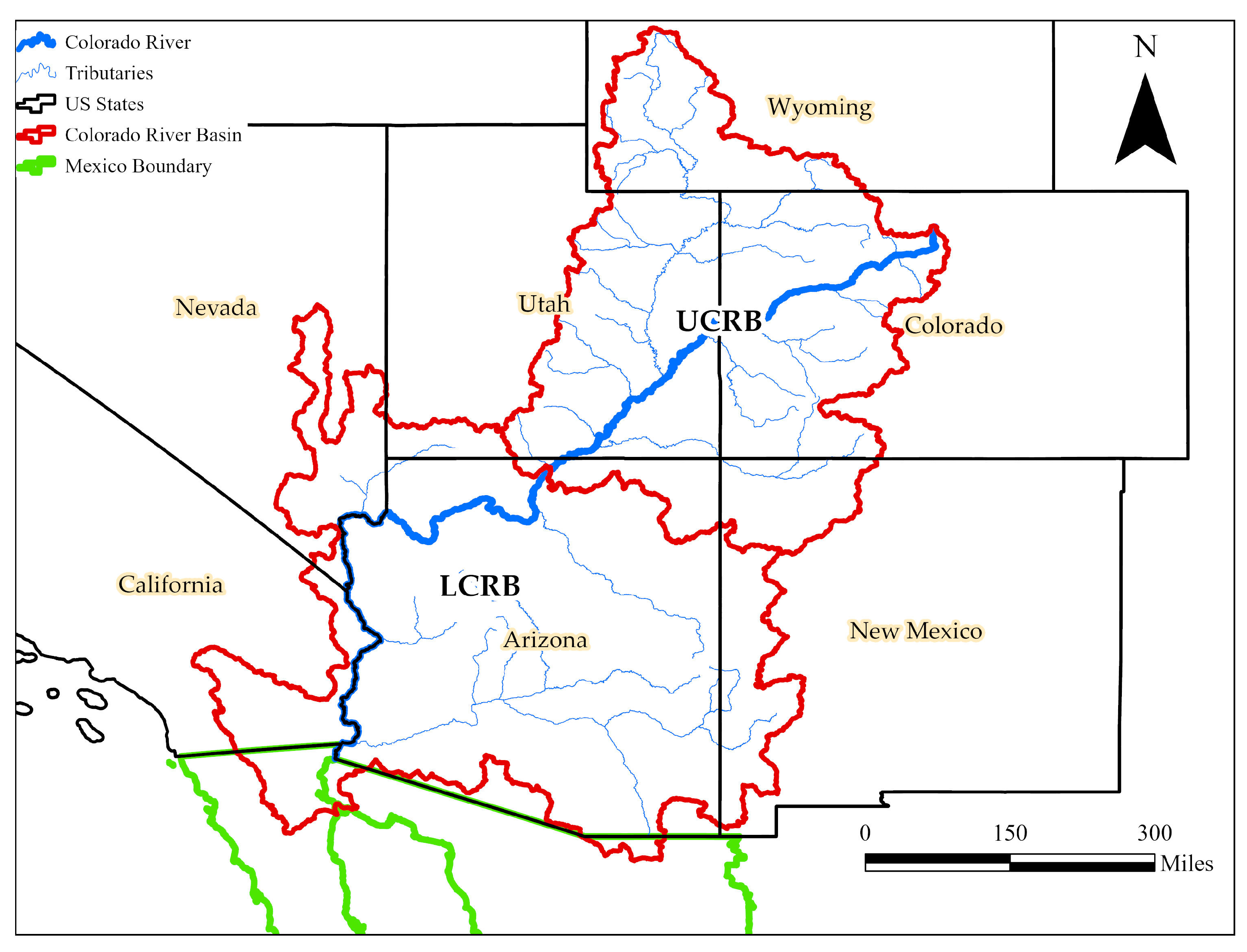
The salt in the Colorado River system is abundant and naturally occurring. A significant number of saline sediments in the CRB were deposited in prehistoric marine conditions. Salts contained in sedimentary rocks are readily erodible, dissolved, and discharged into the river system [25]. In general, the level of salinity in the river increases as it flows downstream with a concentration of about 50 mg/L at its headwaters to about 850 mg/L where it crosses the border between the US and Mexico. On average each year, about nine million tons of salt are carried past the Hoover Dam, which is the uppermost point at which numerical requirements have been established on the river [25,26].

The issues of salinity in the river basin cause annual economic damages in a sum exceeding USD 300 million negatively impacting over 36 million people and 4.5 million acres of irrigated lands [2,5,27,28]. A total of 55% of the dissolved solids in the river basin are accounted for by natural saline springs, natural surface runoff, erosion of saline geologic formations, and groundwater flow. A total of 37% of the salt contributions into the river come from irrigated agricultural lands using both natural and reclaimed wastewater. The remaining 8% of the dissolved solids in the basin are accounted for by evaporative processes and industrial and municipal sources [27,29]. The economic damages caused to the river are estimated to rise to USD 471 million annually by the year 2025 according to the US Bureau of Reclamation [30]. These damages are due to measures put by the US to reduce the TDS load contained in the water discharged to the Republic of Mexico in the international 1944 Water Treaty signed between the two countries [30]. 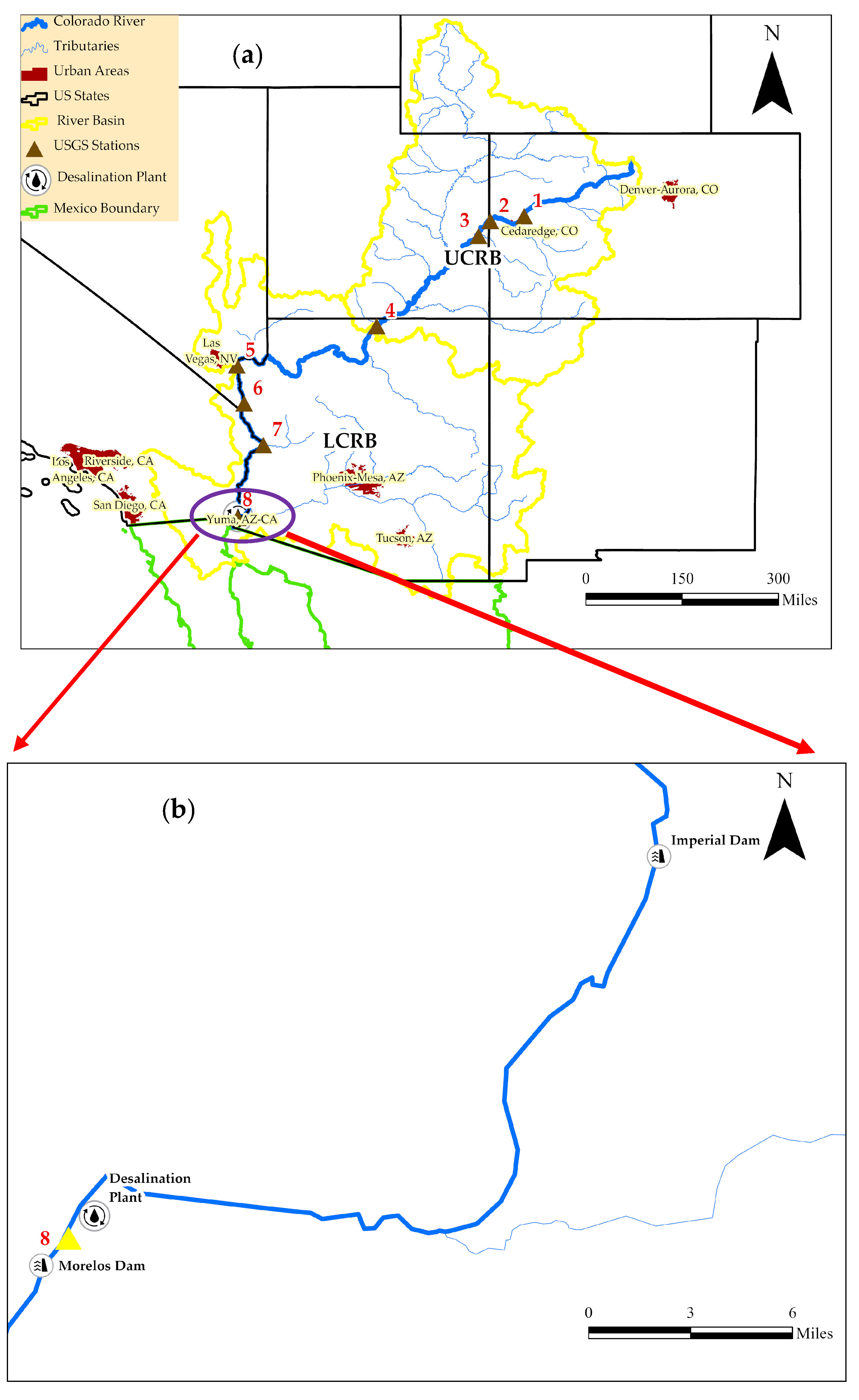The treaty stipulates the delivery of 1.8 billion m³ per year from the Colorado River to the Republic of Mexico in compliance with Minute 242 [28,31]. The CRB Salinity Control Act consequently tasks the Secretaries of the US Department of Agriculture (USDA) and the Department of the Interior to ensure the preservation and safeguarding of the water in the Colorado River. Title I of the Act requires the construction, maintenance, and operation of desalting plants, brine discharge canal, and other facilities to ensure the delivery of water to the Republic of Mexico from the Morelos Dam with a concentration of TDSs no more than 115 ± 30 mg/L above the yearly mean annual flow-weighted TDS concentration which arrives at the Imperial Dam (across the California/Arizona border) of the river. The CRB states adopt different numerical values for TDS concentrations of 879, 747, and 723 (concentrations in mg/L), respectively, for locations below the Imperial, Parker, and Hover Dams [3,25,29].

TSSs consist of organic and inorganic solids suspended in the water columns used in describing sediment pollution in a water body [32]. The average tolerance limit of TSSs in water is about 90 mg/L and 13 mg/L, respectively, for fishes and bottom invertebrates [33]. Only a few states in the US have a numerical criterion set for TSSs with values ranging from 38 to 158 mg/L [33]. TSSs in the Colorado River are impacted by several factors including forest fires, rainfall, and runoff. The occurrence of forest fire events in the upper part of the lower Virgin River watershed is said to have caused drastic changes in the land use and land cover (LULC) leading to erosion of a considerable number of suspended sediments affecting the TSS concentration in Lake Mead located in the Colorado River. Rainfall and associated runoff caused by climate change may also impact the flow of eroded sediments into the river. Heavy rains may generate runoff, which can transport sediments, silt, and pollutants from the land into the river and raise TSS levels. In addition, high precipitation events can result in higher river flows, which might affect the dilution and transport of TDSs and TSSs [34].

TSS accumulation in lakes like those on the Colorado River is likely a phenomenon that requires effective systems to be effectively addressed [35]. Understanding sediment-related issues in freshwater bodies is important as it impacts the quality of the water and subsequently affects the lives of humans and the aquatic ecosystems which depend on these waters for their needs.

TDS and TSS levels in the CRB are influenced by changes in reservoir storage, streamflow, and natural variability in salinity, extraction of energy and mineral resources such as gas, oil, and coal, and agricultural practices. Increased streamflow dilutes the salt in the water. The decline in water level due to evaporation leads to drought in the river and could potentially increase the level of salt in the water. The variations in TDSs and TSSs are strongly influenced by climatic fluctuations in rainfall and snowmelt runoff. Downstream rivers’ water quality variability is changed by reservoir storage. Large reservoirs, such as Lake Powell in the CRB, selectively route less salty water while storing more salty water when flows are low. When inflows start to rise, poor water quality is then released [26,29,36]. TDSs and TSSs related in the basin could not only impair the quality of water in the river basin but also reduce the capacity of reservoirs such as Lake Mead and Lake Powell in the basin for water storage as well as posing operations challenges to the management of the reservoirs in the basin. At the time of their inception, reservoirs had a known amount of water storage capacity. This is however reduced by the mechanism of siltation of the reservoirs by sediments in reservoirs which disrupt the continuous movement of sediments through rivers [37,38]. Sedimentations in reservoirs could lead to reduce usable life and deprives the downstream sections of the river of required sediments necessary for sustenance of aquatic habitats [6,38].

TDS concentrations have a direct impact on groundwater and river bodies worldwide. A high concentration of TDSs has the potential to cause toxicity in aquatic organisms. Changes in the ionic compositions of water and the toxicity of the ions can elevate the salinity of the water which can cause shifts in biotic communities hence limiting their biodiversity [39]. TSSs on the other hand impede light penetration into lower water layers and hence have the potential to cause shallow lakes and bays to silt and smother benthic habitats as they impact both living organisms and eggs. As particles of clay, silt, and other organic materials settle at the bottom of shallow lakes and bays, they have the potential to cause the suffocation of newly hatched larvae and impede the survival of zoobenthos [40]. The presence of TSSs in the water also affects the amount of light that penetrates through the water column which restricts the rate of energy assimilation by benthic algae, macrophytes, and phytoplankton [40]. Improved quantification of TSS and TDS loadings in streams could be useful to assess the possible impacts of urbanized activities such as mining [36]. A TDS/TSS ratio has been proposed as a method for estimating TDS loading using TSSs as an indicator in past studies [36]. Reduction in the biodiversity abundance of aquatic animals in rivers in the North American Great Plains has been linked to changes in hydrology, fragmentation of habitats, and increased concentration of TDSs and TSSs due to associated climate and LULC or landscape use changes [14]. The topography, soil types, and vegetation cover of a local landscape can impact the pace of erosion and sediment transport. The landscape steep slopes and bare and erodible soils can facilitate soil erosion leading to increment in the TSS levels in the river. Studies have found that an increase in sediment loads leads to a decrease in dissolved oxygen which cause affects the development of fish species [14].

Effective monitoring of these WQPs requires a multifaceted approach as no single known approach could efficiently reduce the number of sediments and dissolved solids in one single waterbody. Studies have shown that measures put in place to reduce sediments in the Colorado River could also be beneficial to the reduction of TDSs but only along the reach of the river. Reductions in TSSs could not improve the TDS concentration in tributaries to the Colorado River except for the lower Gunnison and Roaring Fork Rivers [41].

Actions taken to reduce the amount of TSSs and TDSs in the CRB include instituting a water quality control plan to protect and enhance the quality of water in the basin, construction of sediment control measures and best management practices including check dams, erosion control blankets, sediment ponds and traps, and silt fences to contain sediments and prevent their transport during construction works, the implementation of a management plan for non-point source pollution, and instituting salinity control measures by collaborative efforts of the Bureau of Reclamation, Bureau of Land Management, the Basin States Program, and the United States Department of Agriculture (USDA) [25,42,43].

The effectiveness of the management and monitoring efforts of the water systems including rivers and lakes however largely depends on these spatiotemporal changes in the status of these water systems that reflect natural and human activities in the surrounding ecosystems hence the need to carry out this study to understand and provide managers of the river system with insights on the trend of these WQPs in the Colorado River to improve water management practices and to a large extent take measures to ensure the sustainability of the river as a significant source of water for the western US and the Republic of Mexico.

The objective of this study is to analyze the spatiotemporal variations in WQPs specifically TDS and TSS concentrations along the Colorado River. We hypothesized that there is a significant variation in TDS and TSS concentrations along the Colorado River and that the reservoir storage influences the concentrations of these WQPs.

The study subsequently addresses the following questions aimed at achieving the objective:

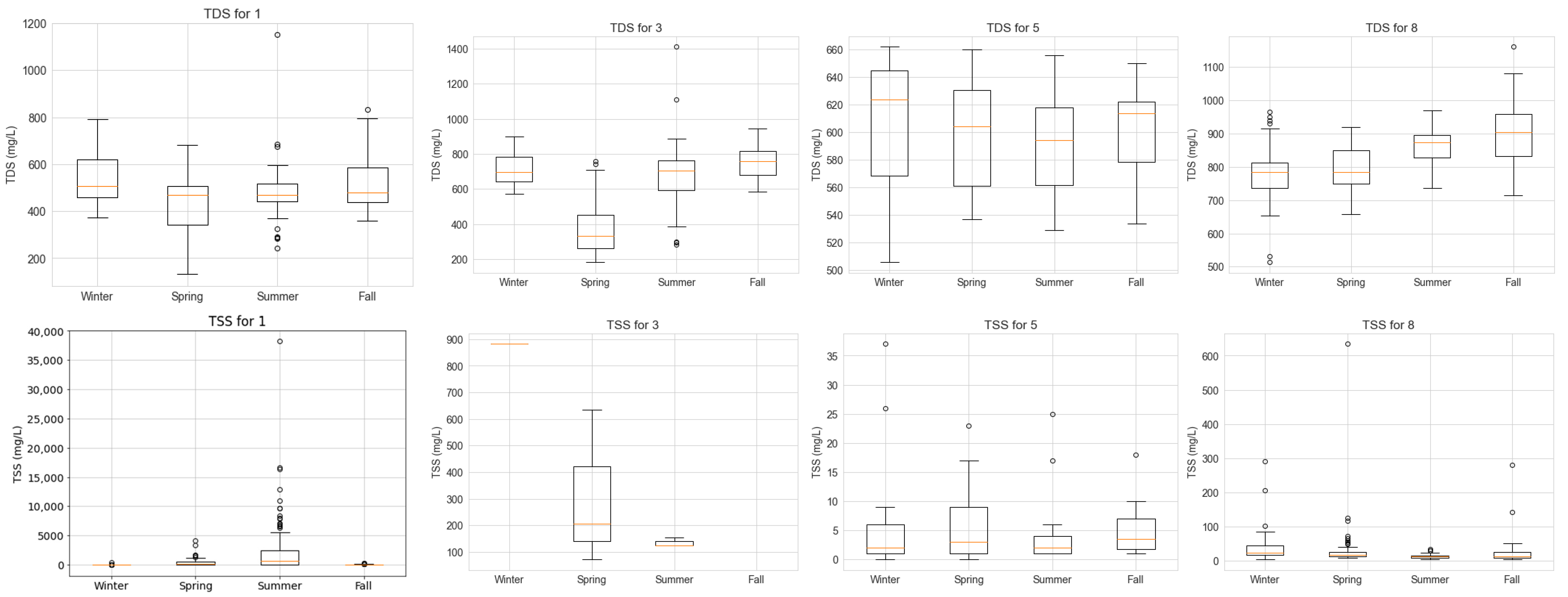
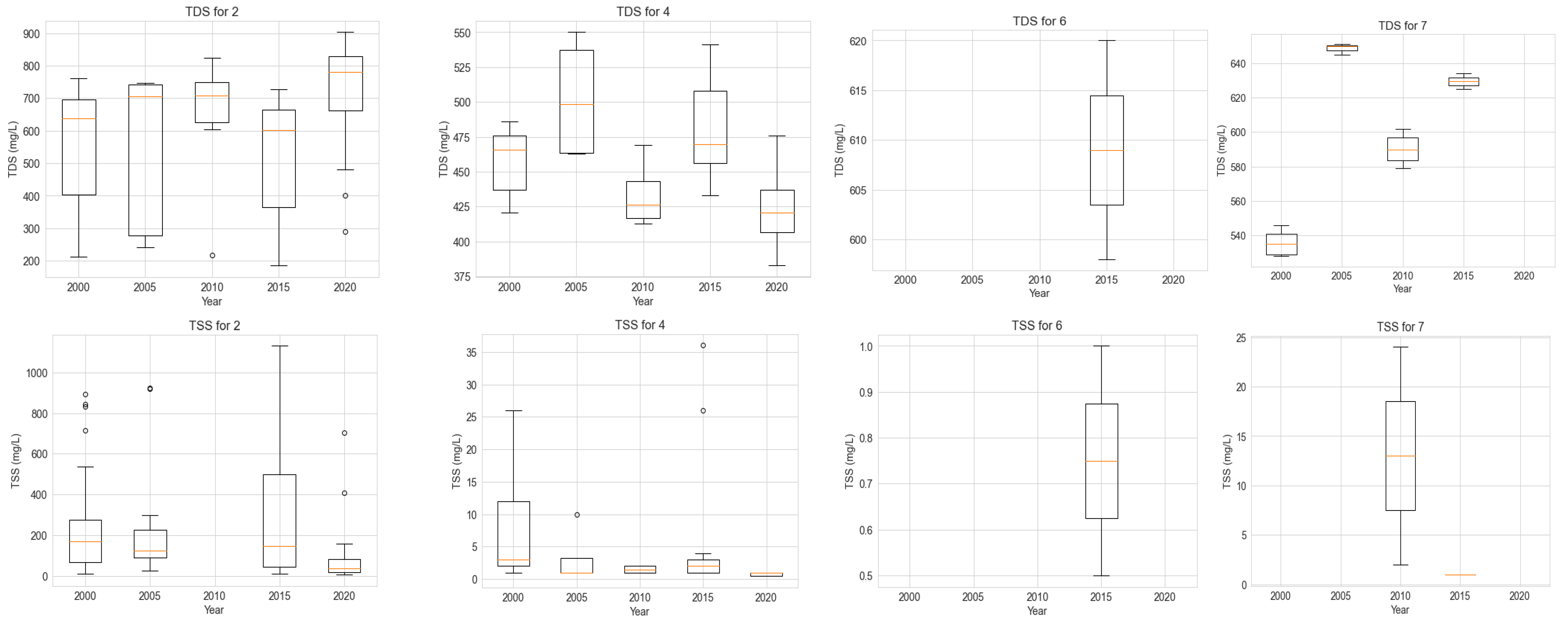
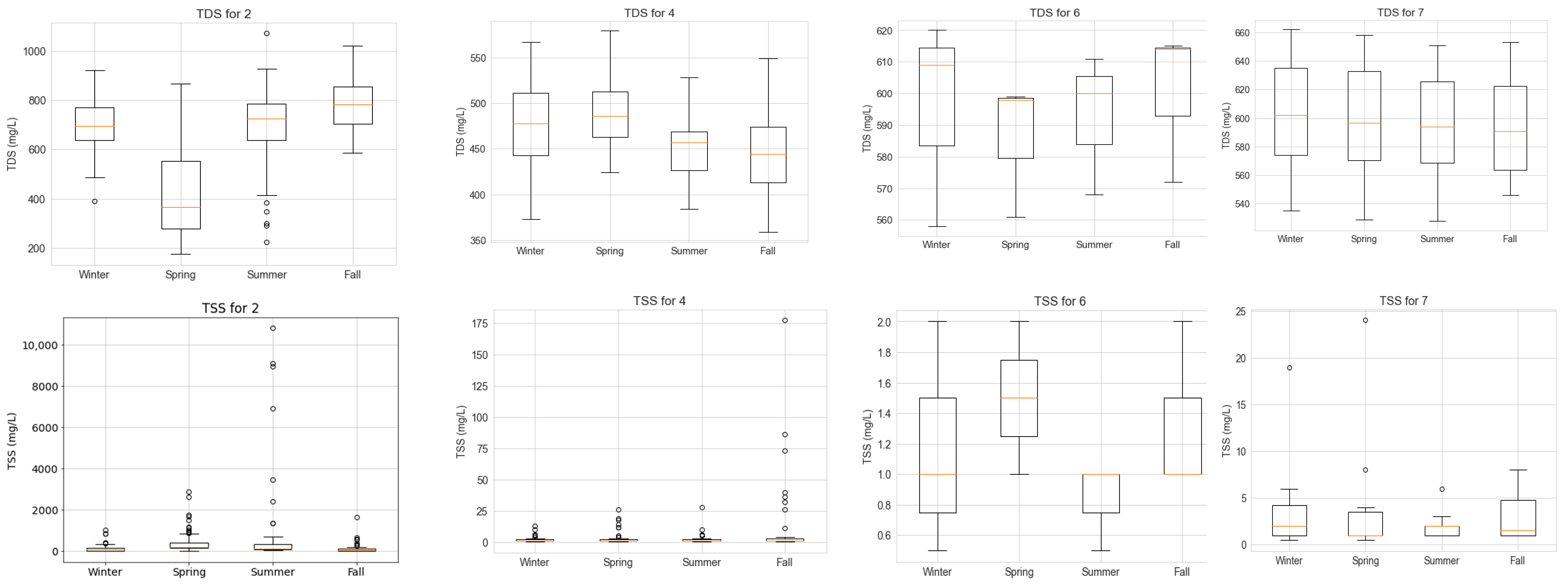
• How do the concentrations of TDSs and TSSs vary spatiotemporally along the Colorado River?
• How do changes in seasons influence the levels of TDSs and TSSs in the Colorado River?
• Is there a statistically significant difference in the TDS and TSS concentrations in the Colorado River in the Upper Colorado River Basin (UCRB) and the Lower Colorado River Basin (LCRB)?

2. Materials and Methods

2.1. Study Area

The Colorado River is housed in the CRB. The Colorado River is about 2318 km long from its headwaters to the mouth located in the Gulf of California with the approximate coordinates of 32° N, 115° W. The river is ranked 6th among 135 rivers in the U.S. with a length of >160.9 km. It is about 15 m wide for its first 80.5 miles and goes to about 61 m wide at the Grand Junction [44]. The river is joined by several tributaries. The major ones include the Yampa, San Juan, Gunnison, White, Delores, Green, Gila, Virgin, and Little Colorado Rivers [44]. The Colorado River is a highly regulated system with a vast network of dams, reservoirs, and aqueducts that divert 90% of the water in the river in the US for municipal and agricultural purposes. The main stem of the river in the US has 15 dams with a combined storage of 71.9 billion m³ [45]. The CRB has an approximate area of about 657,000 sq. km [46]. According to the U.S. Department of the Interior Bureau of Reclamation Upper Colorado Region progress report No. 24, published in 2014, the Colorado River is divided into the Upper and Lower Colorado Basins. The UCRB consists of Colorado, New Mexico, Utah, and Wyoming, while the LCRB consists of Nevada, Arizona, California, and the Gila River between Arizona and New Mexico [29]. The CRB is largely arid to a semi-arid region with elevations varying from sea level to over 4267 m. The basin receives precipitation ranging from 10.16 cm a year in the deserts to up to 152.4 cm a year in some of the upper basin mountainous watersheds. The locations of sub-basins within different climate regimes affect the precipitation. Much of the LCRB is dry because of orographic barriers and persistent high-pressure weather cells. Another factor that influences the changes in precipitation is the changes in elevations of the CRB. There is a wide range of monthly average temperatures in the CRB from below freezing in winter months at upper elevations of the UCRB to nearly over 37.78 °C in summer months in the LCRB. Climatic conditions in the basin are influenced by a sharp climatic gradient and unevenness in topography. Evapotranspiration drives the water cycle in the region. Precipitation evaporates from the soil, snowpack, open water, vegetation, and crops through evapotranspiration [47]. The UCRB has seen a streamflow decline by approximately 20% in the last century based on estimations of naturalized flow above the Lees Ferry. Climate change forces are said to have reduced the streamflow from the UCRB by an approximately 10% with uncertainty reductions at 6–14% [48].

The population growth around the CRB coupled with the irrigation water requirement has led to dramatic stress on the river. The largest reservoirs on the river, namely Lake Mead and Lake Powell, are experiencing a drastic decline in water levels due to intense drought and increased water demand over the last two decades [46,49]. The river and its tributaries provide water to about 35 million people in the US and 3.3 million people in the Republic of Mexico yearly. The river helps maintain the biodiversity of organisms while aiding the economy. Close to 22.3 billion acres and 2.02 billion acres of land in the US and the Republic of Mexico, respectively, obtain their irrigation water supply from Colorado. The river also supports the economy by providing about 16 million jobs with an economic benefit exceeding $1.4 trillion. The basin also provides 4200 MW of electricity to people in the US yearly [26,29,50]. The basin is however, facing drastic water declines leading to increase in stress on the available water due to drought, population growth, over-exploitation of the groundwater aquifers and surface water, and continuous pollution of the freshwater systems, water managers are opting for more sustainable water supply options which save energy which includes desalination of brackish water [51].

The water from the river is allocated by the Colorado River Compact of 1922 and other acts, including the 1928 Boulder Canyon Project Act, the 1944 Water Treaty, the Upper Colorado River Basin Compact of 1948, and rulings by the United States Supreme Court [52]. The Colorado River is considered to be physically, culturally, and economically essential by the twenty-nine (29) federally recognized tribes within the CRB [53]. This study utilizes selected USGS stations on the CRB with the needed TDS and TSS data using the selection criteria described in the data collection section of this document. The map showing the extent of the CRB is presented in Figure 1.

2.2. Data Collection

Water quality data used for inland and coastal waters are available as discrete samples carried through field and laboratory analysis. Professionals and volunteers carry out water quality monitoring programs with higher frequency and near-continuous data using methods such as automated in situ sensors [19].

For this study, in situ water quality data were obtained from the USGS data repository for the river stations from 1 January 2000 to 22 April 2023. The data were retrieved from the USGS website [54]. A search was conducted for the WQPs (field/lab sample data) on the USGS data repository by inputting parameter codes (70301 for TDSs and 80154 for TSSs) for the water quality parameters under consideration for the upper and lower basin hydrological regions as presented in Figure 2. The parameter codes were obtained from the USGS website. The summary approach utilized in the data retrieval is presented in Figure 2. The approximate location, drainage area, and states of the stations with the data for this study are presented in

Table 1. Locations and details of the USGS stations with water quality data used in the study.

No.	Station	Name	State	Basin	Drainage Area (km2)	Lat. (N), Long. (W)
1	9095500	Colorado River near Cameo	CO	UCRB	20,684	39°14′21″, 108°15′56″
2	9163500	Colorado River near Colorado-Utah State Line	CO		46,229	39°07′58″, 109°01′35″
3	9180500	Colorado River near Cisco	UT		62,419	38°48′38″, 109°17′34″
4	9380000	Colorado River at Lees Ferry	AZ	LCRB	289,561	36°51′52″, 111°35′16″
5	9421500	Colorado River below Hoover Dam	NV		444,701	36°00′55″, 114°44′16″
6	9423000	Colorado River below Davis Dam	NV		448,845	35°11′30″, 114°34′17″
7	9427520	Colorado River below Parker Dam	CA		473,191	34°17′44″, 114°08′22″
8	9522000	Colorado River at NIB, above Morelos Dam	AZ		638,950	32°43′07″, 114°43′05″

and further illustrated in Figure 3. The river and tributary shapefile, the basin boundary, and its reservoir storage data were retrieved from the CRB GIS Open Data Portal [55]. A summary of the data availability and period for the station is presented in

Table 2. Data availability for the USGS stations from 2000 to 2023.

	TDS		TSS
Station No.	Period	Count	Period	Count
1	20 January 2000–31 January 2023	339	26 January 2000–14 March 2023	476
2	4 January 2000–14 February 2023	290	4 January 2023–6 September 2022	323
3	29 March 2000–6 April 2022	129	29 March 2000–7 September 2000	7
4	26 January 2000–19 July 2022	197	26 January 2000–14 March 2023	199
5	12 January 2000–24 August 2016	81	20 April 2000–24 August 2016	49
6	14 August 2014–13 May 2019	12	14 August 2014–27 March 2019	11
7	24 January 2000–16 March 2023	70	26 April 2007–14 December 2022	38
8	27 January 2000–14 June 2022	299	27 January 2000–5 December 2022	266

.

The location of the eight sites for the study is presented in Figure 3a to give a geographical representation of the study area. Station 8 (highlighted with a green oval shape) is located above the Morelos Dam where the water is discharged to the Republic of Mexico. Its water quality is therefore important in ensuring compliance with the 1944 Treaty. Above the station is the Yuma Desalting Plant where the water was to be treated before it is channeled to the Morelos Dam for delivery to the Republic of Mexico. The Yuma Desalting Plant is the largest desalination plant in the U.S. owned and managed by the U.S. Bureau of Reclamation constructed in 1974 for the treatment of saline agricultural return flows which arrives from the Welton-Mohawk Irrigation and Drainage District in Arizona into the river before it is delivered to Mexico. The plant can purify about 276,335 m³ of water daily [56,57,58]. The Imperial Dam where the numerical criterion is set is located upstream of the desalination plant as represented in Figure 3b.

2.3. Graphical and Statistical Analysis

The analyses are carried out using graphical technics, descriptive statistics, and inferential statistics.

The findings of this study will aid in understanding the factors influencing the Colorado River’s TDS and TSS levels and informing management plans for protecting and conserving this important resource.

Statistical analyses were conducted utilizing the Python programming version 3.9.12 language employing several libraries and packages such as the NumPy version 1.21.5, Pandas version 1.4.2, and SciPy version 1.7.3. The ESRI ArcGIS Pro software version 3.1.1 was used to create and analyze maps to assess the spatial variations in the WQPs.

2.3.1. Descriptive Statistics

Descriptive statistical methods including measures of central tendency (such as mean) and dispersion (such as standard deviation) were used in analyzing and summarizing the data to aid in understanding the spatiotemporal variability of the data [59,60].

2.3.2. Inferential Statistics

Inferential statistics are performed to test the hypothesis of a study and to make conclusions about the population based on the given data. In this study, analysis of variance (ANOVA) was conducted to check for statistically significant differences in the TDS and TSS concentrations along the river over the studied period. We first checked for the assumptions of the ANOVA test to assess validity and reliability of results using an alpha (α) value of 0.05 [59,61,62,63,64].

3. Results and Discussion

The results obtained from the study to assess the spatiotemporal trends of TDSs and TSSs along the Colorado River are presented and thoroughly discussed in this section of the paper. The results presented provide useful insights into the trends and spatial distribution of TDS and TSS concentrations along the Colorado River.

3.1. Spatiotemporal Trends in the TDSs and TSSs

A summary of the descriptive statistics for the variations of TDS and TSS is presented in

Table 3. Overall summary statistics of TDSs and TSSs at the USGS monitoring stations.

	TDSs (mg/L)				TSSs (mg/L)
Station	Min	Mean	Max	Std	Min	Mean	Max	Std
1	133	488	1150	127	0.5	867	38,200	2579
2	176	621	1070	201	3	360	10,800	1058
3	184	612	1410	218	72	314	882	315
4	359	471	579	44	0.5	5	177	16
5	506	599	662	39	0	6	37	8
6	558	594	620	23	0.5	1.2	2	0.6
7	528	597	662	36	0.5	3	24	5
8	514	820	1160	85	0.4	29	634	49

.

The average TDS concentration for the monitored stations ranges from about 471 mg/L at the Lees Ferry to 820 mg/L recorded above Morelos Dam. The high TDSs recorded above the Morelos Dam could be from saline agricultural return flows from the Welton-Mohawk Irrigation and Drainage District which is a 65,000-acre agricultural area in western Arizona [65,66]. There has been a reported case of deterioration of the river due to the saline drainage water discharged from the wells in the Wellton-Mohawk [67]. The Morelos Dam is a diversion dam with a reduced amount of water and hence less dilution as the water is diverted to Mexico. Less water increases the concentration of dissolved salts. The TDS concentration in the Lees Ferry station is comparatively low compared to other stations which confirms past studies that show a historically low value in this site compared to stations like the Grand Canyon sampling sites. Studies have found studies at the Fees sites to be about 552 mg/L from 1941 to 1968 compared to a 614, 687, and 673 mg/L values recorded at the Grand Canyon, below Hoover Dam Parker, and Parker Dam, respectively [68]. Additionally, the water flows from the Colorado River through the Glen Canyon National Recreation Area located upstream of Lake Mead [69]. The Grand Canyon area is a repository of sedimentary rocks of low dissolved salt contents. The Lees Ferry station is joined by tributaries including the Little Colorado and the Praia Rivers which are known to have little amount of salt concentration. Figure 4a shows the spatial distribution of the TDS concentration along the river. It is seen that highly urbanized areas have high TDS concentrations. The station below may also be impacted by the activities of the residents in a highly urbanized Las Vegas Valley (LVV) which includes the discharge of wastewater from the treatment plants into Lake Mead. The figure shows a general increase of TDSs from the headwaters of the river to its terminus. As the river flows from its headwaters which are rich in minerals, it takes in salt from the river and its tributaries from the UCRB. Some of the tributaries have mean TDS concentrations higher than what is in the main stem river [25]. The return flows from groundwater and drains to the river at the Imperial Dam are said to have higher TDS concentrations than the river due to the sorption of ions from sediments and soils [31]. The waters in the state of Colorado of the CRB are said to be of generally good quality especially those at higher elevations [25] which is confirmed by the results presented in Figure 3a where the first station value was 488 mg/L compared to the 621 mg/L and 612 mg/L recorded for Stations 2 and 3, respectively, which are located in the lower portions of the river in the state. The lower portions of the basin in that state are underlain by bedrock deposits of a cretaceous period which are mostly Mancos Shale and Dakota Sandstone. The Mancos Shale is a marine deposit that constitutes a substantial concentration of easily dissolved substances such as selenium. This selenium is dissolved by groundwater which leaches to the comparatively impermeable shale layers and flows over the bedrock strata toward surface drainages [25].

The average recorded TSS concentration at the monitored stations ranges from about 1 mg/L recorded below the Davis Dam to around 867 mg/L recorded at Station 1 located near Cameo station which is excessively above the maximum 158 mg/L set by the states with the numerical criterion for TSSs. The 867 mg/L value is also beyond the average upper tolerance level for fishes (90 mg/L) and invertebrates (30 mg/L) [33]. Results show a general minimal TSSs in the LCRB compared to the relatively high TSS values in the UCRB as shown in Figure 4b. Unlike TDS, we observe TSS concentration generally reduces as the Colorado River flows from headwaters to its terminus. Most portions of the LCRB show a relatively less amount of sediments due to possibly the existence of numerous reservoirs including Lake Mead and Lake Powell that aid in setting out of the sediments [70] as shown in the difference in the TSS concentrations obtained for the stations presented in Table 3 and Figure 4b. Additionally, the UCRB contains a significant amount of erodible soil that could be transported into the river in the event of rainfall and snowmelts causing a significant hike in the river’s TSS as obtained in Stations 1, 2, and 3. The region is also on high elevations with mountainous terrains and colder temperatures which results in the amount of snow. These snowmelts are a greater contribution to the greater amount of streamflow in rivers. They can therefore be a conduit of increased erosion rates and sediment transports into the river [70,71]. Agricultural practices in the UCRB could also be a significant contributor to TSSs in the river. The byproducts of agriculture practices such as sediments and fertilizers are transported and deposited in the river during rainfall and snowmelt events [25]. The TSSs at Station 8 show a spike compared to other stations in the LCRB possibly due to its highly urbanized area consisting of a large amount of impervious surface which could accelerate the transportation of sediments and soils into the river in a storm event.

3.2. Effects of Reservoir Storage on TDS and TSS Concentrations

Reservoir water storage is crucial for the management of water resources. Reservoirs are sources of steady and reliable water for several uses including irrigation, hydropower generation, and industrial and domestic use. The operation and maintenance of these reservoirs could impact the quality of water. Reservoir storage influences the TDS and TSS concentrations of waterbodies. Reservoirs not only cause considerable damage to the downstream hydrology but also significantly change the variability in the storage salinity. Although reservoir evaporations are reported to be the cause of about 12% of the source of TDSs to the CRB, their overall positive long-term impacts on salinity have significantly decreased salinity peaks and annual fluctuations [29]. Reservoir water storage modifies the fluctuations in the water quality. Reservoirs cause sedimentation and settlement of suspended particles of water which results in a reduction of the water turbidity. Stratification of reservoirs may also cause impairment in the water quality such as low concentrations of DO and high concentrations of hydrogen sulfide, manganese, and iron [72].

We assess the impact of reservoir storage on the TDS and TSS concentrations by plotting the average reservoir storage for four reservoirs namely Lake Mead, Lake Powell, Lake Mohave, Lake Havasu, the Granby Dam, and the Morelos Diversion Dams together with the average concentrations of the WQPs along the river as shown in Figure 5. From Figure 5a,b, we can see that the variability in the TDS and TSS concentrations is potentially impacted by the reservoir storage. The TDS concentration appears to be increasing as the river flows into Lake Powell, but with the storage of the lake we see a drastically changed in concentration from 612 to 471 mg/L for TDSs and a dramatical change of TSSs from 314 to 5 mg/L. These concentrations slightly increased as the water moves into the Lake Mead area. The flows may have picked up a significant amount of sediments and dissolved mineral salts as they transport them from the UCRB into Lake Mead. The lake storage could be a significant factor for seeing only a slight increment from Lake Powell. The concentrations were further slightly reduced to Lake Havasu but increased quite significantly above the Morelos Dam after the desalting plant. Runoffs into the river from agricultural non-point sources and highly urbanized tributaries could be responsible for the elevated TDS and TSS concentrations at the station above the Morelos Dam. The plant constructed to treat agriculture runoff and save Lake Mead’s water was only operational three times after its construction in 1992 due to operational cost (USD 55.2 million) for operating the plant for full capacity and for long-term and technical problems including five design deficiencies. More 2743 m of aluminum–bronze pipes require replacement [73,74]. Studies have attributed reservoirs to playing a significant role in retaining the inflow of dissolved solids. An estimated 10% of the inflow of dissolved solids were said to have been retained in Lake Mead [50].

3.3. Assessing the Seasonal and Yearly Variations in TDSs and TSSs

The time series of the TDS and TSS concentrations for the studied period (2000–2023) is presented in Figure 6 to assess the temporal variation of the WQPs. It is observed from Figure 6a that there are variations in the TDS concentrations with Station 8 showing generally higher concentrations. The level of TDS increases from Station 1 near Cameo to Station 8 below the Morelos Dam, an indication of the rise in TDS from upstream of the river to downstream as described in Section 3.1. There are year to year variations in the amounts of TDS for the studied period highlighting the impacts of the watershed activities of the period with an unusual dramatic rise in the TDS concentration in Station 3 near Cisco, located in Grand County, Utah, during the years 2012/2013. The spike in the TDS in the years 2012/13 could be due to intense snowmelt that year coupled with anthropogenic activities such as agriculture. The Colorado River near Cisco received flows from the Dolores and San Miguel Rivers. The Dolores River flows about 240 miles and drains an arid region of the Colorado Plateau. The San Miguel River joins the Dolores River which flows into the Colorado River. The headwaters of the Dolores River are traced to the San Juan Mountains which is known to be a great spot for fishing for several kinds of trout [75]. These rivers are potential sources of increased dissolved salts in the Colorado River. The TSSs appear to be relatively low for all the stations except for Stations 1 and 2. Stations located below or above show relatively low concentrations of TSSs indicating the direct influence of storage on the settling and sedimentations of suspended solids. USGS Station 2 is found to be the significant source of TSSs for the Colorado River over the studied period except in 2021 where there was a spike in the TSSs from Station 1 possibly due to an unusual snowmelt which increased the flow and transportation of sediments into the river. Station 2, located near Colorado–Utah state line, receives flow from the Gunnison River which is one of the major tributaries of the Colorado River [44]. The tributary contributes about one-third of Colorado’s flow at the state line station. Flows from the Gunnison River move through a steep-gradient, narrow Black Canyon channel located in the Gunnison National Park which is a possible conduit of loaded sediments in the Colorado River [76]. The station also receives flow from the urbanized Grand Junction, CO, located in Mesa County with highly impervious surfaces which could accelerate the transport of sediments into the river. Grand Junction’s primary industry before the discovery of its mineral riches was agriculture. The mining of the deposits of coal, radium, copper, uranium, and vanadium and the operations of the mining activities [77] could be significant contributors to the release of sediments to the Colorado River raising the TSS concentrations at USGS Station 2.

Boxplots were also used to visualize and compare the spread of the yearly distribution of TDS and TSS concentrations for selected stations (Stations 1 and 3 in the UCRB and 5 and 8 in the LCRB) as presented in Figure 7 for years divisible by 5. Seasonal variations for the TDSs and TSSs are also presented in

Table 4. Overall mean seasonal statistics of TDS and TSS at the USGS monitoring stations.

	TDS (mg/L)				TSS (mg/L)
Station	Winter	Spring	Summer	Fall	Winter	Spring	Summer	Fall
1	541	475	432	516	5	309	1866	72
2	745	521	541	771	84	395	340	631
3	716	482	550	762	-	575	116	124
4	452	495	461	461	3	3	2.4	17
5	599	605	594	599	3	11	5	5
6	618	582	594	593	1	2	9	1.5
7	605	601	595	580	4	5	2	2.2
8	832	765	841	901	29	41	15	24

and Figure 8. The findings for the rest of the stations (Stations 2, 4, 6, and 7) are also presented as appendices in Appendix A (Figure A1 and Figure A2). From the boxplots, we can see that monitoring efforts are less frequent as compared to those of TDSs possibly because TDSs are a threatening issue in the basin with an annual estimate of economic damage exceeding USD 300 million [41].

The results in Table 4 show that the maximum TDS level is at Station 8 regardless of the season of the year indicating that activities around the area of the basin have a huge impact on the TDSs. Station 8 is also the terminus of the river and a repository of dissolved minerals and salts carried from upstream of the river. A critical study of the results did not however show a general increment or decrement of TDSs and TSSs in each season along the river although it follows a similar pattern as presented in Figure 4, an indication that the cause of TDSs and TSSs to the river is multifaceted and cannot directly be traced to one known source.

The highest TDS concentration of 901 mg/L was in fall at Station 8 with the least TDSs recorded at Station 1 in summer with the highest TSSs of 1866 mg/L recorded at Station 1 in summer and the least TSSs also at Station 6. It can therefore be inferred that during the summer when snowmelts are high, TDS concentrations are generally low, but TSS concentration spikes, particularly in non-reservoir stations. This is not the case in reservoir stations as there is high evaporation during the summer coupled with high consumptive use during the summer period. The increased temperature during the summer and fall months results in an increment in the evaporation rate which could impact the TDS levels [78]. Studies have found evaporation rates to be higher during fall months even when flow declines [79] which potentially explains the high TDS values obtained at Station 8 during the fall season. In general, we observed variability in TDSs across the seasons with higher concentrations observed in the winter and fall seasons. Higher flow rates during the spring and summer and increased precipitations and snowmelt runoff can dilute the concentrations of TDSs which is evident in the results presented in Table 4. Conversely, there is a reduction in TSSs during the winter and fall seasons due to low runoff and snowmelts as compared to the spring and summer months. TDS concentrations in the LCRB are slightly higher than those in the UCRB while TSSs in the LCRB are lower than those in the UCRB. Both basins present distinctively different terrains, LULC, and practices as discussed in Section 3.4.

The box denotes the interquartile range (IQR) of the WQPs while the whiskers are extensions within 1.5 times the IQR. The DOTs represent outliers (values outside the whiskers). These plots are useful in evaluating and interpreting patterns relating to the spatiotemporal variations in these WQPs and have been used in several studies [80,81]. Results shown in the box plot follow a similar pattern as described by the time series analysis and in Section 3.1. with the whiskers showing huge variability possibly due to differences in the occurrences such as rainfall and snowmelt in the years and seasons. The seasonal boxplots for TDSs and TSSs in Figure 7 and Figure 8 show that the variations in these WQPs are accounted for by several factors including agriculture and irrigation activities, particularly in the summer and fall seasons. Some of the stations had no data for some years and hence have empty boxplots for those years as seen in the figures.

In summary, TDS levels across various stations and years show a variety of behavioral patterns. While some stations’ TDS levels fluctuate over time, others display numbers that are quite consistent with Station 8 consistently showing TDS values above the recommended EPA guidelines of 500 mg/L. While stations showed relatively consistent levels of TSSs, others such as Stations 1 and 2 exhibit sporadic changes over the period. The data analyzed do not show a clear general trend of improving or worsening TDSs or TSSs at the locations of the studied period. The findings highlight the significance in carrying out station-specific analysis to assess the variations in these WQPs as different stations may be subjected to the influx of the different environmental conditions. The absence of consistent and uniform patterns in the WQPs across all the station is an indication that factors restricted to the locality such as LULC, local geology, streamflow, and human activities compounded by drought events are crucial in controlling the levels of these WQPs in the basin [29,47,50]. Analysis was made on the data that are currently available which have some limitations including data gaps especially for the case of TSS which poses the challenge of drawing detailed and concrete deductions from the analysis. There is therefore a need for extensive and continuous monitoring programs to close these gaps and advance our overall knowledge of water quality for environmental health and water resources sustenance. Additionally, the data used span several years making it crucial to consider various contributing elements such as droughts, local events, and climatic variations that could affect trends in water quality. Further studies will need to quantify the impact of drought induced changes to these WQPs.

3.4. Detection of Significance Levels in TDS and TSS Trends Using Inferential Statistics

We applied inference statistics to check for any significant differences in the WQPs station to station, basin to basin, month to month, season to season, and year to year.

3.4.1. ANOVA Test

Results from the assumption test of ANOVA are presented in

Table 5. Test of Assumptions for the WQPs.

	Shapiro–Wilk Normality Test		Levene Homogeneity of Variance Test
WQPs	Statistics	p-value	Statistics	p-value
TDS	0.988	0.000	60.012	0.000
TSS	0.227	0.000	10.573	0.000

for the test of Normality and Levene Homogeneity of Variance. We conducted the Shapiro–Wilk Normality Test to check if the WQPs are normally distributed and the Levene Homogeneity Test to check for homogeneity of variance in the WQPs. TDS and TSS data collected meet the assumption of independence of observations since they were collected at different sites or locations with each observation distinctively different from others. We formulated a null hypothesis (Ho) that TDS and TSS are each normally distributed. The alternate hypothesis (H₁) was that these WQPs are not normally distributed. To check for the assumption of homogeneity of variance, we hypothesized that the variance of groups of the TDS and TSS are equal was used. The H₁ was that the variances of TDS and TSS groups are not equal [59,60,61,63,82].

Results in Table 5 show a p-value of both TDSs and TSSs as less than the α level (0.05) for both normality and the homogeneity tests showing that the Ho for the presence of normality and the homogeneity of variance is not met. The null hypotheses are therefore rejected which indicates a violation of the assumptions underlying the ANOVA test.

3.4.2. Kruskal–Wallis Test

We conducted a non-parametric test since the assumption is not met for the ANOVA. We conducted the non-parametric Kruskal–Wallis test to check for statistical significance differences in the monthly, seasonal, and yearly WQPs [83]. The Kruskal–Wallis test, which has been used in many studies including those in engineering and the social sciences, compares the groups using rank sums rather than the means as in the case of ANOVA. To identify any significant differences in the medians, the test computes the sum of ranks for each group after rating the observations within each group [59,84,85]. Results of the analysis for WQPs are presented in

Table 6. Kruskal–Wallis test for the monthly WQP significance test.

	TDSs		TSSs
Month	Statistics	p-Value	Statistics	p-Value
1	1.647	0.200	1.494	0.222
2	2.548	0.110	2.926	0.087
3	4.392	0.036	9.433	0.002
4	26.458	0.000	5.000	0.025
5	0.071	0.790	9.377	0.002
6	5.870	0.015	26.740	0.000
7	10.620	0.001	0.329	0.566
8	1.842	0.175	0.029	0.865
9	0.260	0.610	11.773	0.001
10	0.138	0.710	3.959	0.047
11	0.420	0.517	0.946	0.331
12	0.030	0.862	1.040	0.308

,

Table 7. Kruskal–Wallis test for the seasonal WQP significance test.

	TDSs		TSSs
	Statistics	p-Value	Statistics	p-Value
Winter	411.00	0.491	340.00	0.490
Spring	417.00	0.491	412.00	0.491
Summer	306.00	0.489	369.00	0.490
Fall	279.00	0.489	244.00	0.488

and

Table 8. Kruskal–Wallis test for the yearly WQP significance test.

	TDS		TSS
Year	Statistics	p-Value	Statistics	p-Value
2000	72.00	0.478	66.00	0.477
2005	38.00	0.469	25.00	0.462
2010	45.00	0.472	25.00	0.462
2015	83.00	0.479	73.00	0.478
2020	70.00	0.476	61.00	0.476

.

Results shown in Table 6 show that there is a statistically significant difference within March, April, June, and July for TDS concentrations and within March, April, June, September, and October for TSS concentrations which is an indication that these parameters are impacted by the onset of seasonal factors like snowmelt runoff, monsoon rainfalls, and evaporations in these months. It is however worth noting that the Kruskal–Wallis test is unable to identify the locations of occurrence of stochastic dominance or the number of groups in the dominance. Further analysis is however required to better understand the complex interactions between the TDS and TSS concentrations and the water management and natural process impacting the quality of the Colorado River each month [86] as well as the exact impact of urbanizations and anthropogenic activities on these WQPs in the river [87].

Results presented in Table 7 and Table 8 show there is no statistically significant differences in TDS and TSS concentrations within each of the four seasons (winter, spring, summer, and fall) and within the years of study at an α-level of 0.05 which is an indication of the consistent influence of TDS and TSS concentrations by the factors affecting these WQPs within each season and year along the Colorado River.

We also performed statistical significance tests across the months, seasons, and years for the TDS and TSS concentrations and presented the results in

Table 9. Kruskal–Wallis test WQP significance test across the months, seasons, and years.

	TDSs		TSSs
	Statistics	p-Value	Statistics	p-Value
Month	159.42	0.000	172.20	0.000
Season	117.07	0.000	154.77	0.000
Year	54.63	0.000	290.36	0.000

. The results show that there are statistically significant differences in TDS and TSS from month to month, season to season, and year to year. These significant variations are largely due to seasonal rises in consumptive use, agriculture practices, snowmelts runoffs, and evaporation rates exacerbated by increased temperature in the summer months [79] and summer recreational activities. There are distinctive differences in the occurrences and activities in seasons in the basin which influence the WQPs differently. Winter periods are generally characterized by lower temperatures and rainfalls. Temperatures rise during the spring and peak in the summer and subsequently start to drop in the fall. Increased temperatures increase the evaporative rates which affect the dissolved contents, particularly in reservoirs in the river. Spring is characterized by rises in runoff and streamflow which may lead to a greater amount of TSSs in the river.

We compared the TDS and TSS concentration between the basins (for all data combined, by months, seasons, and years) and found that there is a statistically significant difference in the levels of TDSs and TSSs between the UCRB and LCRB as shown in

Table 10. Significance test between the basins.

	TDS		TSS
	Statistics	p-Value	Statistics	p-Value
Together	0.58	0.447	822.84	0.000
Month	357.32	0.000	935.73	0.000
Season	191.64	0.000	902.82	0.000
Year	170.80	0.000	904.39	0.000

which may be due to several plausible reasons including but not limited to (i) streamflow: the LCRB has a lot of reservoirs that release flows into the lower section of the river. These flows dilute the TDS concentrations. Lake Powell was filled for the first time in 1983, but it spilled. This spill went through Lake Mead. Flows in the lake were however unusually high and sustained from 1983 to 1987 causing record-low levels of TDSs [29]. (ii) Reservoir storage: large reservoirs selectively channel less salty water during low inflows while retaining more saline water. The saline water is subsequently slowly released after the inflows start to rise [29]. (iii) Agriculture activities: agriculture-related irrigation is the largest user of the basin water use and a huge contributor of salinity to the river. Irrigated lands in the UCRB have been found to contribute an estimated 3.4 million tons of salt to the river per year. Agricultural activities in the UCRB could also increase the deposit of sediments in the river. Additionally, there is a difference in the geology between the UCRB and LCRB which may play a significant role in the transport of sediments. The UCRB is on mountainous terrain with high elevations consisting of different vegetation and soils which may end up being deposited into the river [5]. (iv) Energy development: The exploitation of energy resources, notably oil shale, coal, gas, oil, gas, and coal bed methane, particularly in the UCRB, is a potential contributor to the TDS levels in the river. Mineral dissolution could cause an increment in the salinity of surface waters [29].

We also assessed the significant level of TDSs and TSSs for each basin (for all data combined, by months, seasons, and years) as presented in

Table 11. Significance test within the basins.

		TDSs		TSSs
		Statistics	p-Value	Statistics	p-Value
UCRB	Month	285.60	0.000	101.89	0.000
	Season	161.23	0.000	171.28	0.000
	Year	102.55	0.000	36.11	0.015
LCRB	Month	14.52	0.206	27.10	0.004
	Season	2.31	0.679	8.38	0.079
	Year	94.19	0.000	75.63	0.000

and found there was a statistically significant difference in TDSs and TSSs within the UCRB. The monthly and seasonal TDS and seasonal TSS however show no significant variation in the LCRB. The trend in the LCRB could be the presence of reservoirs and the spikes in anthropogenic activities at some locations in the basin such as the Welton-Mohawk Irrigation and Drainage District [65,66].

4. Conclusions

The study aimed to assess the spatiotemporal trends of TDSs and TSSs along the Colorado River, which is a major source of water to the western US and the Republic of Mexico with its headwaters originating from the Rocky Mountains in Colorado and running into its terminus at the northern part of the Gulf of California. The analysis conducted shows that the TDS concentration was significantly higher in the UCRB while the LCRB shows a generally high level of TSS. We found that the activities in these two basins are distinctive and may be a factor in these variations. While the UCRB is characterized by mountainous terrain producing large amounts of snow melt and an increase in agriculture, mining, and energy development activities, the LCRB is made of several large reservoirs including Lake Mead and Lake Powell with huge storage which have the potential to effectively dilute the effects of dissolved salts. These reservoirs, however, experienced large evaporations during the summertime which plays significant impacts on their TDS level. The byproducts of agriculture and mining practices such as sediments and fertilizers are transported and deposited in the river during rainfall and snowmelt, increasing the level of TSSs particularly in the UCRB. Additionally, TSSs in the river basin are increased by natural erosion from neighboring watersheds which are aided by slope steepness and the LULC of the region as well as channel and streambank erosion of the river basin.

The study also examines the statistical significance of these WQPs within and across months, seasons, and years and between the basins using the Kruskal–Wallis test. Results from the significance test show there are statistically significant differences in TDSs and TSSs from month to month, season to season, and year to year. We suspect that these significant variations are largely due to the prolong drought in the basin leading to seasonal rises in consumptive use as well as agriculture practices, snowmelt runoff, and evaporation rates exacerbated by increased temperature in the summer months [31,47,79]. It is however worth noting that the Kruskal–Wallis test is unable to identify the locations of the occurrence of stochastic dominance in the levels of TDSs and TSSs.

In summary, this study presents detailed findings in understanding the spatiotemporal variability of the TDS and TSS concentration along the Colorado River which can help water management and conservation authorities to develop efficient strategies to lessen the detrimental effects of prolonged drought, natural variations such as precipitation, snowmelts, and runoff, and anthropogenic activities on the basin’s water quality. Further research may examine the relationship between TDS and TSS concentrations and other WQPs to gain more knowledge about the overall condition of the river ecosystem. Additional research will need to be conducted to quantify the effect of flowrates, precipitation, LULC, channel modifications, and evaporation on the overall changes TDS and TSS concentration in the river system.

References

1. Adjovu, G.E.; Ahmad, S.; Stephen, H. Analysis of Suspended Material in Lake Mead Using Remote Sensing Indices. World Environ. Water Resour. Congr. 2021, 2021, 754–768. [Google Scholar] [CrossRef]
2. Adjovu, G.E.; Stephen, H.; Ahmad, S. Monitoring of Total Dissolved Solids Using Remote Sensing Band Reflectance and Salinity Indices: A Case Study of the Imperial County Section, AZ-CA, of the Colorado River. World Environ. Water Resour. Congr. 2022, 2022, 1132–1145. [Google Scholar] [CrossRef]
3. Venkatesan, A.K.; Ahmad, S.; Batista, J.R.; Johnson, W.S. Total Dissolved Solids Contribution to the Colorado River Associated with the Growth of Las Vegas Valley. In Proceedings of the World Environmental and Water Resources Congress 2010: Challenges of Change, Providence, RI, USA, 16–20 May 2010; pp. 3376–3385. [Google Scholar] [CrossRef]
4. Hart, R.J.; Hooper, R.P. Monitoring the Water Quality of the Nation’s Large Rivers. Available online: https://pubs.usgs.gov/fs/fs-014-00/ (accessed on 28 May 2023).
5. Nauman, T.W.; Ely, C.P.; Miller, M.P.; Duniway, M.C. Salinity Yield Modeling of the Upper Colorado River Basin Using 30-m Resolution Soil Maps and Random Forests. Water Resour. Res. 2019, 55, 4954–4973. [Google Scholar] [CrossRef]
6. Wheeler, K.G.; Udall, B.; Wang, J.; Kuhn, E.; Salehabadi, H.; Schmidt, J.C. What Will It Take to Stabilize the Colorado River? Science 2022, 377, 373–375. [Google Scholar] [CrossRef] [PubMed]
7. De Vlaming, V.; DiGiorgio, C.; Fong, S.; Deanovic, L.A.; De La Paz Carpio-Obeso, M.; Miller, J.L.; Miller, M.J.; Richard, N.J. Irrigation Runoff Insecticide Pollution of Rivers in the Imperial Valley, California (USA). Environ. Pollut. 2004, 132, 213–229. [Google Scholar] [CrossRef]
8. Kimbrough, R.A.; Litke, D.W. Pesticides in Streams Draining Agricultural and Urban Areas in Colorado. Environ. Sci. Technol. 1996, 30, 908–916. [Google Scholar] [CrossRef] [Green Version]
9. Schliemann, S.A.; Grevstad, N.; Brazeau, R.H. Water Quality and Spatio-Temporal Hot Spots in an Effluent-Dominated Urban River. Hydrol. Process. 2021, 35, e14001. [Google Scholar] [CrossRef]
10. Song, K. Water Quality Monitoring Using Landsat Themate Mapper Data with Empirical Algorithms in Chagan Lake, China. J. Appl. Remote Sens. 2011, 5, 053506. [Google Scholar] [CrossRef]
11. Stout, W.L.; Fales, S.L.; Muller, L.D.; Schnabel, R.R.; Elwinger, G.F.; Weaver, S.R. Assessing the Effect of Management Intensive Grazing on Water Quality in the Northeast U.S. J. Soil Water Conserv. 2000, 55, 238–243. [Google Scholar]
12. Usali, N.; Ismail, M.H. Use of Remote Sensing and GIS in Monitoring Water Quality. J. Sustain. Dev. 2010, 3, 228–238. [Google Scholar] [CrossRef]
13. Masocha, M.; Murwira, A.; Magadza, C.H.D.; Hirji, R.; Dube, T. Remote Sensing of Surface Water Quality in Relation to Catchment Condition in Zimbabwe. Phys. Chem. Earth 2017, 100, 13–18. [Google Scholar] [CrossRef]
14. Mueller, J.S.; Grabowski, T.B.; Brewer, S.K.; Worthington, T.A. Effects of Temperature, Total Dissolved Solids, and Total Suspended Solids on Survival and Development Rate of Larval Arkansas River Shiner. J. Fish Wildl. Manag. 2017, 8, 79–88. [Google Scholar] [CrossRef] [Green Version]
15. Salmaso, N.; Mosello, R. Limnological Research in the Deep Southern Subalpine Lakes: Synthesis, Directions and Perspectives. Adv. Oceanogr. Limnol. 2010, 1, 29–66. [Google Scholar] [CrossRef]
16. Fant, C.; Srinivasan, R.; Boehlert, B.; Rennels, L.; Chapra, S.C.; Strzepek, K.M.; Corona, J.; Allen, A.; Martinich, J. Climate Change Impacts on Us Water Quality Using Two Models: HAWQS and US Basins. Water 2017, 9, 118. [Google Scholar] [CrossRef] [Green Version]
17. Oun, A.; Kumar, A.; Harrigan, T.; Angelakis, A.; Xagoraraki, I. Effects of Biosolids and Manure Application on Microbial Water Quality in Rural Areas in the US. Water 2014, 6, 3701–3723. [Google Scholar] [CrossRef] [Green Version]
18. Lee, S.; Ahn, K.H. Monitoring of COD as an Organic Indicator in Waste Water and Treated Effluent by Fluorescence Excitation-Emission (FEEM) Matrix Characterization. Water Sci. Technol. 2004, 50, 57–63. [Google Scholar] [CrossRef]
19. El Serafy, G.Y.H.; Schaeffer, B.A.; Neely, M.; Spinosa, A.; Odermatt, D.; Weathers, K.C.; Baracchini, T.; Bouffard, D.; Carvalho, L.; Conmy, R.N.; et al. Integrating Inland and Coastal Water Quality Data for Actionable Knowledge. Remote Sens. 2021, 13, 2899. [Google Scholar] [CrossRef] [PubMed]
20. Dube, T.; Mutanga, O.; Seutloali, K.; Adelabu, S.; Shoko, C. Water Quality Monitoring in Sub-Saharan African Lakes: A Review of Remote Sensing Applications. Afr. J. Aquat. Sci. 2015, 40, 1–7. [Google Scholar] [CrossRef]
21. Khan, I.; Khan, A.; Khan, M.S.; Zafar, S.; Hameed, A.; Badshah, S.; Rehman, S.U.; Ullah, H.; Yasmeen, G. Impact of City Effluents on Water Quality of Indus River: Assessment of Temporal and Spatial Variations in the Southern Region of Khyber Pakhtunkhwa, Pakistan. Environ. Monit. Assess. 2018, 190, 267. [Google Scholar] [CrossRef]
22. Adjovu, G.E.; Stephen, H.; James, D.; Ahmad, S. Overview of the Application of Remote Sensing in Effective Monitoring of Water Quality Parameters. Remote Sens. 2023, 15, 1938. [Google Scholar] [CrossRef]
23. American Public Health Association; American Water Works Association; Water Environment Federation. Standard Methods for The Examination of Water and Wastewater; Baird, R.B., Eaton, A.D., Rice, E.W., Eds.; American Public Health Association: Washington, DC, USA, 2017; pp. 1–1545. [Google Scholar]
24. Sowby, R.B.; Hotchkiss, R.H. Minimizing Unintended Consequences of Water Resources Decisions. J. Water Resour. Plan. Manag. 2022, 148, 02522007. [Google Scholar] [CrossRef]
25. Colorado River Basin Salinity Control Forum 2020 Review: Water Quality Standards for Salinity, Colorado River System. 2020. Available online: https://coloradoriversalinity.org/docs/2020%20REVIEW%20-%20Final%20w%20appendices.pdf (accessed on 28 May 2023).
26. Tillman, F.D.; Anning, D.W. A Data Reconnaissance on the Effect of Suspended-Sediment Concentrations on Dissolved-Solids Concentrations in Rivers and Tributaries in the Upper Colorado River Basin. J. Hydrol. 2014, 519, 1020–1030. [Google Scholar] [CrossRef]
27. Shope, C.L.; Gerner, S.J. Assessment of Dissolved-Solids Loading to the Colorado River in the Paradox Basin between the Dolores River and Gypsum Canyon, Utah; U.S. Department of the Interior, US Geological Survey: Salt Lake City, UT, USA, 2016; pp. 1–18. [Google Scholar]
28. Tillman, F.D.; Day, N.K.; Miller, M.P.; Miller, O.L.; Rumsey, C.A.; Wise, D.R.; Longley, P.C.; McDonnell, M.C. A Review of Current Capabilities and Science Gaps in Water Supply Data, Modeling, and Trends for Water Availability Assessments in the Upper Colorado River Basin. Water 2022, 14, 3813. [Google Scholar] [CrossRef]
29. Bureau of Reclamation. Quality of Water; Progress Report No. 24.; U.S. Department of the Interior and Bureau of Reclamation: Washington, DC, USA, 2013; pp. 1–124. Available online: https://www.usbr.gov/uc/progact/salinity/pdfs/PR24final.pdf (accessed on 28 May 2023).
30. Venkatesan, A.K.; Ahmad, S.; Johnson, W.; Batista, J.R. Salinity Reduction and Energy Conservation in Direct and Indirect Potable Water Reuse. Desalination 2011, 272, 120–127. [Google Scholar] [CrossRef]
31. Cederberg, J.R.; Paretti, N.V.; Coes, A.L.; Hermosillo, E.; Lucia, A. Estimation of Dissolved-Solids Concentrations Using Continuous Water-Quality Monitoring and Regression Models at Four Sites in the Yuma Area, Arizona and California, January 2017 through March 2019; U.S. Geological Survey: Reston, AZ, USA, 2021; pp. 1–26. [Google Scholar] [CrossRef]
32. Sagan, V.; Peterson, K.T.; Maimaitijiang, M.; Sidike, P.; Sloan, J.; Greeling, B.A.; Maalouf, S.; Adams, C. Monitoring Inland Water Quality Using Remote Sensing: Potential and Limitations of Spectral Indices, Bio-Optical Simulations, Machine Learning, and Cloud Computing. Earth-Science Rev. 2020, 205, 103187. [Google Scholar] [CrossRef]
33. US EPA Office of Water and Office of Science and Technology. US EPA Developing Water Quality Criteria for Suspended and Bedded Sediments (SABS). 2003. Available online: https://archive.epa.gov/epa/sites/production/files/2015-10/documents/sediment-report.pdf (accessed on 28 May 2023).
34. Imen, S.; Chang, N.B.; Yang, Y.J. Developing the Remote Sensing-Based Early Warning System for Monitoring TSS Concentrations in Lake Mead. J. Environ. Manag. 2015, 160, 73–89. [Google Scholar] [CrossRef]
35. Edalat, M.M.; Stephen, H. Socio-Economic Drought Assessment in Lake Mead, USA, Based on a Multivariate Standardized Water-Scarcity Index. Hydrol. Sci. J. 2019, 64, 555–569. [Google Scholar] [CrossRef]
36. Butler, B.A.; Ford, R.G. Evaluating Relationships between Total Dissolved Solids (TDS) and Total Suspended Solids (TSS) in a Mining-Influenced Watershed. Mine Water Environ. 2018, 31, 18–30. [Google Scholar] [CrossRef]
37. Bid, S.; Siddique, G. Identification of Seasonal Variation of Water Turbidity Using NDTI Method in Panchet Hill Dam, India. Model. Earth Syst. Environ. 2019, 5, 1179–1200. [Google Scholar] [CrossRef]
38. Kondolf, G.M.; Gao, Y.; Annandale, G.W.; Morris, G.L.; Jiang, E.; Zhang, J.; Cao, Y.; Carling, P.; Fu, K.; Guo, Q.; et al. Sustainable Sediment Management in Reservoirs and Regulated Rivers: Experiences from Five Continents. Earth’s Futur. 2014, 2, 256–280. [Google Scholar] [CrossRef]
39. Weber-Scannell, P.K.; Duffy, L.K. Effects of Total Dissolved Solids on Aquatic Organisms: A Review of Literature and Recommendation for Salmonid Species. Am. J. Environ. Sci. 2007, 3, 1–6. [Google Scholar] [CrossRef] [Green Version]
40. Giardino, C.; Brando, V.E.; Dekker, A.G.; Strömbeck, N.; Candiani, G. Assessment of Water Quality in Lake Garda (Italy) Using Hyperion. Remote Sens. Environ. 2007, 109, 183–195. [Google Scholar] [CrossRef]
41. Tillman, F.D.; Anning, D.W.; Heilman, J.A.; Buto, S.G.; Miller, M.P. Managing Salinity in Upper Colorado River Basin Streams: Selecting Catchments for Sediment Control Efforts Using Watershed Characteristics and Random Forests Models. Water 2018, 10, 676. [Google Scholar] [CrossRef] [Green Version]
42. California Regional Water Quality Control Board; Colorado River Basin Region State Water Resources Control Board. Colorado River Basin Region Water Quality Control Plan for the Colorado River Basin. Available online: https://www.waterboards.ca.gov/coloradoriver/water_issues/programs/basin_planning/docs/2020/rb7bp_e2019.pdf (accessed on 28 May 2023).
43. Colorado Department of Transportation. Chapter 5 Construction Control Measures. 2019. Available online: https://www.codot.gov/programs/environmental/landscape-architecture/erosion-control-stormwater-quality-1/erosion-storm-quality/chapter-5 (accessed on 28 May 2023).
44. U.S. Department of the Interior; U.S. Geological Survey. River Basins of the United States: The Colorado. Available online: https://pubs.usgs.gov/gip/70039371/report.pdf (accessed on 28 May 2023).
45. Anning, D.W.; Coes, A.L.; Mason, J.P. Conceptual and Numerical Models of Dissolved Solids in the Colorado River, Hoover Dam to Imperial Dam, and Parker Dam to Imperial Dam, Arizona, California, and Nevada; U.S. Geological Survey: Reston, VA, USA, 2018. [Google Scholar]
46. Rahaman, M.; Thakur, B.; Kalra, A.; Ahmad, S. Modeling of GRACE-Derived Groundwater Information in the Colorado River Basin. Hydrology 2019, 6, 19. [Google Scholar] [CrossRef] [Green Version]
47. Lukas, J.; Payton, E. Colorado River Basin Climate and Hydrology: State of the Science; Western Water Assessment; Western Water Assessment, University of Colorado Boulder, Cooperative Institute for Research in Environmental Science: Boulder, CO, USA, 2020; ISBN 1219950920. [Google Scholar] [CrossRef]
48. Hoerling, M.; Barsugli, J.; Livneh, B.; Eischeid, J.; Quan, X.; Badger, A. Causes for the Century-Long Decline in Colorado River Flow. J. Clim. 2019, 32, 8181–8203. [Google Scholar] [CrossRef]
49. Adjovu, G.E.; Ali Shaikh, T.; Stephen, H.; Ahmad, S. Utilization of Machine Learning Models and Satellite Data for the Estimation of Total Dissolved Solids in the Colorado River System. Proceedings of the World Environmental and Water Resources Congress 2023 1147–1160. [CrossRef]
50. Rumsey, C.A.; Miller, O.; Hirsch, R.M.; Marston, T.M.; Susong, D.D. Substantial Declines in Salinity Observed Across the Upper Colorado River Basin During the 20th Century, 1929–2019. Water Resour. Res. 2021, 57, e2020WR028581. [Google Scholar] [CrossRef]
51. Shrestha, E.; Ahmad, S.; Johnson, W.; Shrestha, P.; Batista, J.R. Carbon Footprint of Water Conveyance versus Desalination as Alternatives to Expand Water Supply. Desalination 2011, 280, 33–43. [Google Scholar] [CrossRef]
52. Venkatesan, A.K.; Ahmad, S.; Johnson, W.; Batista, J.R. Systems Dynamic Model to Forecast Salinity Load to the Colorado River Due to Urbanization within the Las Vegas Valley. Sci. Total Environ. 2011, 409, 2616–2625. [Google Scholar] [CrossRef]
53. Bureau of Reclamation. Colorado River Basin SECURE Water Act Section 9503(c) Report to Congress; U.S. Department of the Interior: Washington, DC, USA, 2021; pp. iii-25. Available online: https://www.usbr.gov/climate/secure/docs/2021secure/basinreports/ColoradoBasinChapter.pdf (accessed on 28 May 2023).
54. U.S. Department of the Interior; U.S. Geological Survey. National Water Information System: Web Interface. Available online: https://waterdata.usgs.gov/nwis/qw (accessed on 28 May 2023).
55. The Babbitt Center for Land and Water Policy. Colorado River Basin GIS Open Data Portal. Available online: https://coloradoriverbasin-lincolninstitute.hub.arcgis.com/ (accessed on 28 May 2023).
56. Piper Hansen Cronkite News. Despite One Plant’s Failure, Desalination Works. Arizona Capitol Times, 27 February 2022. Available online: https://azcapitoltimes.com/news/2022/02/27/despite-one-plants-failure-desalination-works/(accessed on 28 May 2023).
57. Bureau of Reclamation. Yuma Desalting Plant. Available online: https://www.usbr.gov/lc/yuma/facilities/ydp/yao_ydp.html (accessed on 28 May 2023).
58. Holmes, C. Why an Arizona Desalination Plant Has Been Idle for 30 Years. abc 15 Arizona. 2022. Available online: https://www.abc15.com/news/region-central-southern-az/yuma/why-an-arizona-desalination-plant-has-been-idle-for-30-years (accessed on 28 May 2023).
59. Adjovu, G.E. Evaluating the Performance of A GIS-Based Tool for Delineating Swales Along Two Highways in Tennessee. Master’s Thesis, ProQuest LLC, Ann Arbor, MI, USA, 2020. [Google Scholar]
60. Mishra, P.; Pandey, C.M.; Singh, U.; Gupta, A.; Sahu, C.; Keshri, A. Descriptive Statistics and Normality Tests for Statistical Data. Ann. Card. Anaesth. 2019, 22, 67–72. [Google Scholar] [CrossRef]
61. Kim, H. Analysis of Variance (ANOVA) Comparing Means of More than Two Groups. Restor. Dent. Endod. 2014, 7658, 74–77. [Google Scholar] [CrossRef] [PubMed] [Green Version]
62. Hidayati, N.F.; Rahman, M.; Fauzana, N.A.; Aisiah, S. Effectiveness of Chitosan To Reduce the Color Value, Turbidity, and Total Dissolved Solids in Shrimp-Washing Wastewater. Russ. J. Agric. Socio-Econ. Sci. 2021, 115, 82–88. [Google Scholar] [CrossRef]
63. Kim, T.K. Understanding One-Way Anova Using Conceptual Figures. Korean J. Anesthesiol. 2017, 70, 22–26. [Google Scholar] [CrossRef] [PubMed] [Green Version]
64. Suharini, E.; Ariyadi, M.H.; Kurniawan, E. Google Earth pro as a Learning Media for Mitigation and Adaptation of Landslide Disaster. Int. J. Inf. Educ. Technol. 2020, 10, 820–825. [Google Scholar] [CrossRef]
65. Marin, C. A Report on Colorado River Salinity Operations, Under International Boundary and Water Commission Minute No 242. 2007. Available online: https://www.ibwc.gov/Files/Web/Annual_CO_Salinity_Report-2005.pdf (accessed on 28 May 2023).
66. McMurrray, C. The Colorado River Basin and Climate: Perfect Storm for the Twenty-First Century ? Available online: https://www.coloradocollege.edu/dotAsset/74e91de4-a1ff-4062-b628-030e997b4e0b.pdf (accessed on 28 May 2023).
67. Hem, J. Study and Interpretation of the Chemical Characteristics of Natural Water; Department of the Interior, US Geological Survey: Alexandria, VA, USA, 1985. [Google Scholar]
68. Slawson, G.C. Water Quality in the Lower Colorado River and the Effect of Reservoirs. 1972. Available online: https://repository.arizona.edu/bitstream/handle/10150/626787/azu_td_hwr_0102_sip1_w.pdf?sequence=1&isAllowed=y (accessed on 28 May 2023).
69. Ferrari, R.L. 2001 Lake Mead Sedimentation Survey 2001. 2008. Available online: https://www.usbr.gov/lc/region/g2000/LakeMeadSedimentationSurvey2001.pdf (accessed on 28 May 2023).
70. Colorado River Basin Salinity Control Forum. 2017 Review Water Quality Standards for Salinity Colorado River System. 2017. Available online: https://www.coloradoriversalinity.org/docs/2017%20Review%20-%20FINAL.pdf (accessed on 28 May 2023).
71. U.S. Department of the Interior; U.S. Geological Survey. Snowmelt Runoff and the Water Cycle. 2019. Available online: https://www.usgs.gov/special-topics/water-science-school/science/snowmelt-runoff-and-water-cycle (accessed on 28 May 2023).
72. Herschy, R.W. Water Quality in Lakes and Reservoirs; Encyclopedia of Earth Sciences Series; Springer Science+Business Media B.V.: Berlin, Germany, 2012; ISBN 9781402044106. [Google Scholar] [CrossRef]
73. Sandler, G. Yuma Plant Meant to Conserve Water will Cost Millions to Update. Available online: https://cronkitenews.azpbs.org/2018/05/02/yuma-plant-meant-to-conserve-water-will-cost-millions-to-update/ (accessed on 28 May 2023).
74. Udasin, S. Could Desalination Play a Role in the Colorado River Basin’s Future? Pinal Central, 15 January 2022. Available online: https://www.pinalcentral.com/arizona_news/could-desalination-play-a-role-in-the-colorado-river-basin-s-future/article_55f4f881-073d-50b2-9954-c4a0d2bb92e4.html(accessed on 28 May 2023).
75. Uncover Colorado. Dolores River—Near Dolores. Available online: https://www.uncovercolorado.com/activities/dolores-river/ (accessed on 28 May 2023).
76. Holm, H. Gunnison River. Colorado Encyclopedia. Available online: https://coloradoencyclopedia.org/article/gunnison-river (accessed on 28 May 2023).
77. Ike. Mining History in Mesa County. Mesa County Libraries, 1 May 2016. Available online: https://mesacountylibraries.org/2016/05/mining-history-in-mesa-county/(accessed on 28 May 2023).
78. O’Connor, D.J. Seasonal and Long-Term Variations of Dissolved Solids in Lakes and Reservoirs. J. Environ. Eng. 1989, 115, 1213–1234. [Google Scholar] [CrossRef]
79. Earp, K.J.; Moreo, M.T. Evaporation from Lake Mead and Lake Mohave, Nevada and Arizona, 2010–2019; US Geological Survey: Reston, VA, USA, 2021. [Google Scholar]
80. Hajigholizadeh, M. Water Quality Modelling Using Multivariate Statistical Analysis and Remote Sensing in South Florida. Ph.D. Thesis, Florida International University, Miami, FL, USA, 2016. Available online: https://digitalcommons.fiu.edu/etd/2992 (accessed on 28 May 2023).
81. Saher, R.; Stephen, H.; Ahmad, S. Effect of Land Use Change on Summertime Surface Temperature, Albedo, and Evapotranspiration in Las Vegas Valley. Urban Clim. 2021, 39, 100966. [Google Scholar] [CrossRef]
82. Ghasemi, A.; Zahediasl, S. Normality Tests for Statistical Analysis: A Guide for Non-Statisticians. Int. J. Endocrinol. Metab. 2012, 10, 486–489. [Google Scholar] [CrossRef] [Green Version]
83. Zhang, Z.; Zhang, F.; Du, J.; Chen, D.; Zhang, W. Impacts of Land Use at Multiple Buffer Scales on Seasonal Water Quality in a Reticular River Network Area. PLoS ONE 2021, 16, e0244606. [Google Scholar] [CrossRef]
84. Pérez-Gutiérrez, J.D.; Paz, J.O.; Tagert, M.L.M. Seasonal Water Quality Changes in On-Farm Water Storage Systems in a South-Central U.S. Agricultural Watershed. Agric. Water Manag. 2017, 187, 131–139. [Google Scholar] [CrossRef] [Green Version]
85. Giao, N.T.; Van Cong, N.; Nhien, H.T.H. Using Remote Sensing and Multivariate Statistics in Analyzing the Relationship between Land Use Pattern and Water Quality in Tien Giang Province, Vietnam. Water 2021, 13, 1093. [Google Scholar] [CrossRef]
86. Wikipedia®. Kruskal—Wallis One-Way Analysis of Variance. Available online: https://en.wikipedia.org/wiki/Kruskal–Wallis_one-way_analysis_of_variance (accessed on 28 May 2023).
87. Shaikh, T.A.; Adjovu, G.E.; Stephen, H.; Ahmad, S. Impacts of Urbanization on Watershed Hydrology and Runoff Water Quality of a Watershed: A Review. In Proceedings of the World Environmental and Water Resources Congress 2023, Henderson, NV, USA, 21–24 May 2023; pp. 1271–1283. [Google Scholar] [CrossRef]
Figure 1. Map of the Colorado River Basin with Surrounding States created in the ESRI ArcGIS Pro software.
Hydrology 10 00125 g001
Figure 2. Schematic approach for the retrieval of water quality from the USGS data repository.
Hydrology 10 00125 g002
Figure 3. Map showing the locations of USGS stations along the Colorado River produced in the ESRI ArcGIS Pro software. (a) shows the distribution of stations while (b) shows the details of surrounding features (i.e., dams and the desalination plant) of Station 8 marked with yellow triangle symbol.
Hydrology 10 00125 g003
Figure 4. Spatial Distribution of the mean TDSs (a) and TSSs (b) along the Colorado River.
Hydrology 10 00125 g004
Figure 5. Spatial Distribution of the average reservoir storage and mean TDSs (a) and TSSs (b) along the Colorado River.
Hydrology 10 00125 g005
Figure 6. Time series variations of TDS (a) and TSS (b) concentration at the sampling locations along the Colorado River.
Hydrology 10 00125 g006aHydrology 10 00125 g006b
Figure 7. Boxplots showing the yearly distribution of TDS and TSS concentration for each USGS station over the studied period along the Colorado River.
Hydrology 10 00125 g007
Figure 8. Boxplots showing the seasonal distribution TDS and TSS concentration for each USGS station over the studied period along the Colorado River.
Hydrology 10 00125 g008