Monte Carlo Simulations as an Alternative for Solving Engineering Problems in Environmental Sciences: Three Case Studies

Abstract

Monte Carlo methods offer a fast, cost-effective approach for modeling environmental systems influenced by random variability. This study applied them to three abiotic cases: (I) water quality in a lentic surface water source, (II) sizing of a homogenization chamber for solid waste treatment, and (III) removal of atmospheric particulate matter by rain. Deterministic models produced wide and inconsistent estimates: BOD₅ concentrations from 5.28 to 19.81 mg/L (275% relative difference), chamber volumes from 24.12 to 116.53 m³, and particulate matter reductions with up to 60 µg/m³ per month variation. Monte Carlo simulations, by contrast, captured system variability and provided more robust outputs: a design value of 94.84 m³ for the homogenization chamber, narrower ranges for BOD₅, and realistic distributions of atmospheric PM concentrations. Results show that reliance on average values introduces strong biases and mathematical incompatibilities, while the Monte Carlo approach yields quantitative predictions that are both accurate and operationally useful. This confirms its relevance as a practical tool for analyzing and designing environmental systems under uncertainty.

1. Introduction

Environmental sciences are an interdisciplinary academic field integrating physical, biological, chemical, engineering, and mathematical sciences with the aim of studying the environment and solving environmental problems through mathematical models, predictions, and experimentation [1,2,3]. The field of Environmental Science gained prominence during the 1960s and 1970s in response to the need for a multidisciplinary approach to tackle complex environmental issues.

Given the broad scope of environmental sciences, there is no single methodology for research, teaching, or knowledge creation. Instead, this field incorporates and adapts diverse tools and approaches from other scientific disciplines. One widely used strategy is mathematical modeling, which has become increasingly relevant in applied sciences and engineering [4,5]. In environmental research, interest in mathematical modeling has also grown significantly. Scopus, a database widely recognized for its comprehensive coverage of scientific and academic literature [6], reports nearly 6000 publications containing “environment” AND “mathematical modeling” in their titles, abstracts, or keywords over the last two decades. Figure 1 shows the steady increase in the number of publications, highlighting both the relevance of this topic and the growing interest of the scientific community. This upward trend is consistent with the bibliometric study by [7], which analyzed the use of mathematical tools for understanding environmental phenomena based on records from the Web of Science database.

Environmental systems can be classified as biotic, abiotic or mixed systems. This study focuses on abiotic systems, which are modeled by integrating matter and energy balances, transfer phenomena of heat, mass, and momentum, as well as thermodynamic equilibrium laws. These models often result in complex systems of equations (algebraic and/or differential) and logical conditions that can hardly be solved analytically, which hinders the ability to study phenomena under different conditions [8,9,10,11,12].

Traditionally, mathematical models (MMs) in environmental sciences have been extensively used to address a variety of applications, including, global change, pollution control, wastewater treatment, soil decontamination, air quality monitoring, and the sustainable management of natural resources [13,14,15,16,17,18]. Due to the ever-expanding knowledge of environmental systems, modern environmental models have become increasingly intricate, incorporating numerous variables and interdependent systems. This complexity necessitates the use of numerical methods for solving the complex equations within these models [19,20,21].

Mathematical models (MMs) used in environmental sciences can be classified into several types depending on the nature of the variables, the mathematical approach employed, and their behavior, as proposed by Nirmalakhandan [9]. According to this classification, the first subdivision of MMs is based on the degree of certainty. When the variables and their changes are well defined, the relationships among them are fixed, and the results are unique; such models are deterministic. Conversely, if randomness or uncertainty is associated with at least one variable or the results, the model is considered stochastic. Deterministic MMs are typically constructed using algebraic or differential equations, whereas stochastic MMs incorporate statistical characteristics, such as probability distributions. Among the latter, Monte Carlo (MC) methods are particularly noteworthy [5,9,22,23].

The application of MC methods across scientific fields has demonstrated their success in solving complex mathematical models. These methods offer versatility, enabling the analysis of models with random variables and the simulation of diverse scenarios. However, the applicability of MC simulations in environmental engineering and sciences has yet to be fully explored and evaluated, particularly as a more accessible and affordable alternative for academic, scientific, and operational purposes [24,25]. Some examples of MC methods have been applied to environmental sciences for evaluating environmental degradation [23], eutrophication of water bodies [26], simulate phthalate concentrations in university campuses [27] or to model the ozone concentration over various Chinese cities [28].

This paper proposes the use of MC simulations as a fast, cost-effective, and easy-to-implement alternative for the cited purposes, that is for academic, scientific, and operational applications in solving mathematical models of abiotic environmental systems. To demonstrate this approach, three case studies will be developed: (I) modeling the organic load of a lentic surface water source, (II) determining the required volume for a homogenization chamber at a solid waste treatment center, and (III) simulating the elimination of a specific contaminant from the atmosphere by rain. The presented case studies demonstrate the applicability of MC methods to both static MMs, represented by an algebraic equation (case II), and dynamic models, ranging from a single ODE (case I) to a system of ODEs (case III). This application underscores the versatility of MC methods in addressing a wide spectrum of challenges in environmental modeling.

2. Methodology

The methodology for addressing each case study followed a structured approach based on the Modeling Cycle proposed by Henry O. Pollak [20] (see Figure 2). This framework allowed for a systematic examination of the environmental problems posed in the study. For each case, the process began with a clear definition of the variables involved, their behavior, and the boundaries of the problem. All case studies presented in this work are based on computational simulations designed to represent hypothetical environmentally relevant scenarios. These simulations model the behavior and dispersion of pollutants in solid, liquid, and gaseous phases, reflecting a range of contamination challenges. Furthermore, the mathematical complexity of the models varies across cases, encompassing both algebraic equations and differential equations to accurately capture the dynamics of each environmental system.

The case studies are briefly described here with a more in-depth description of each in the results section:

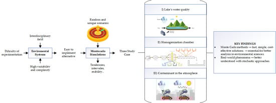
• Case I: A 10 km³ lake receives river water with an average flow of 10 m³/s and a BOD₅ concentration of 20 mg/L. The lake volume remains constant, and outflow BOD₅ matches the lake’s concentration. An industrial company begins discharging variable-flow, high-organic-load wastewater into the lake, impacting water quality over time.
• Case II: At a Solid Waste Treatment Plant operating from 08:00 to 16:00, garbage is unloaded into a storage pit, which ensures continuous feed to the process. A crane transfers the waste to conveyor belts leading to manual sorting, where recyclables are removed. The remaining waste passes through a screening drum that separates organics for composting, while the rest is sent to a landfill.
• Case III: Downtown air is continuously polluted by particulate matter (PM) from mobile sources. Due to its small size, PM stays suspended for long periods. Rain can help remove PM through washout, but rain droplets may also evaporate upon contact with hot vehicle-emitted particles, reducing this effect.

Following this, for cases I and II the mathematical model was derived using the general material balance equation, establishing the logical conditions for each scenario, whereas for case III a model proposed by Shukla et al. (2008) [29] was studied. The subsequent step involved developing a solution algorithm tailored to each model, ensuring accurate simulations. Finally, the outcomes were analyzed through a series of steps, including range delimitation, determining the optimal number of iterations, and conducting MC simulations. This comprehensive approach enabled a robust analysis of the response variables, further supported by statistical validation tests.

The three case studies were modeled using an MC approach; the methodology proposed by Marc Bouissou [30], with modifications made by Taco-Mena et al. [31], was implemented to determine the optimal number of scenarios or iterations.

For each case study, simulations were conducted until the observed fluctuation in the estimated quantity of interest stabilized or until the total accumulated error was less than 3%. This was done by simulating a number of iterations in base ten (1–10–100–1000–10,000–100,000, etc. iterations). For each iteration value, 10 repetitions were performed. The results obtained were tabulated, and the accumulated error was calculated using the following Equation (1):

$$\%error=100\sum _i^1\sum _j^1{\displaystyle \frac{\left|a_{ij}-\overline{a}\right|}{\overline{a}}}$$

(1)

where $a_{ij}$ is the value of the variable of interest in iteration $i$ and repetition $j$, and $\overline{a}$ is the average value of the variable.

Simulations were performed on Matlab 2024a^® and calculations were executed using commercial personal computers (Processor Intel (R) Core (TM) i7-10510U CPU @ 1.80 GHz, 2304 Mhz, 4 cores, 8 GB of RAM), with simulation times less than 1 min for all cases. For Cases I and III times were selected to observe steady-state conditions, whereas for Case II time was selected from knowledge of a real-world plant.

For each case normality tests such as the Anderson-Darling test, the Jarque–Bera test, and the Lilliefors test were conducted to assess normality of the distributions [32].

The Anderson–Darling (A–D) test evaluates the fit of a sample to a specified distribution by measuring the squared distance between the empirical and theoretical cumulative distribution functions, with extra weight given to the tails. The Jarque–Bera (J–B) test assesses normality by combining measures of sample skewness and kurtosis into a statistic that, under the null hypothesis of normality, follows a chi-square distribution with two degrees of freedom. The Lilliefors test is a variant of the Kolmogorov–Smirnov test for normality applicable when the population mean and variance are unknown and estimated from the data; it uses simulation-based critical values to account for these estimations.

3. Results and Discussion

3.1. Case Study I: Modeling the Concentration of BOD₅ in a Lentic Surface Water Source

3.1.1. Description and Conditions of the Case Study I

A lake with a defined volume of 10 km³ receives water from a river with an average flow rate of 10 m³/s and a BOD₅ concentration of 20 mg/L. The river flow varies due to rainfall conditions. The water exits the lake through a second river with a BOD₅ concentration equal to that of the lake. The changes in the lake’s volume are negligible. At a certain point, an industrial company begins operations in the area and discharges wastewater with a high organic load directly into the lake. The flow and BOD₅ concentration of the discharge vary depending on the company’s activities over a defined time interval. A schematic representation of this scenario is shown in Figure 3.

The goal is to model the change in concentration of BOD₅ in the lake over a 20-year period under the conditions outlined in

Table 1. Conditions of Case Study I.

Conditions	Description
Initial conditions	Before the company started its activities, the BOD5 concentration in the lake was in equilibrium with the river under non-rain conditions.
Variability of environmental conditions	Rainfall in the river’s drainage area has been recorded for 20% of the days in a given year, increasing the total river flow by 10–50% during rainfall events. The net organic load (mg/L·s) contributed by the river is constant and does not depend on rainfall events; thus, the dilution effect on the inlet concentration must be considered.
Variability of discharge properties	The flow rate and the pollutant load of the company’s discharge are variables and can be described by probability distributions: flow rate *N (500, 25) L/s and BOD5 concentration *U (360, 980) mg/L.
Organic load decomposition	The lake undergoes a first-order degradation process for organic matter, as commonly reported in the literature [33].
Water flow	Evaporation or diffusion effects are neglected but inflow from rainfall events is considered, with a 20% likelihood of occurrence. There are no changes in water density, and the sum of the inlet flows equals the outlet flow.

* N (µ, σ): Normal distribution with mean µ and standard deviation σ; * U (li, ls): Uniform distribution with lower limit li and upper limit ls.

and determine if the discharge will have a perceptible impact on the dynamics of the water source.

3.1.2. Mathematical Model for Case Study I

The mathematical model used for Case Study I is based on material balance equations.

The general material balance equation is applied to the BOD₅ load in the lake:

$$Input + Generation = Output + Accumulation$$

(2)

The input is the BOD₅ load entering through the river and the company’s discharge, expressed as:

$${Input=Q}_{in}{C}_{in}+Q_v{C}_v$$

(3)

where $Q$ represents the flow rate, $C$ represents the BOD₅ concentration, and the subscripts “$in$” and “$v$” refer to the river and the discharge, respectively.

The generation term, associated with the BOD₅ degradation, is given by:

$$Generation=-kCV$$

(4)

where $k$ is the kinetic constant, $C$ is the lake’s BOD₅ concentration, and $V$ is the total volume of the lake.

The output term is expressed as:

$$Output =Q_{out}C$$

(5)

where $Q_{out}$ represents the output flow rate from the lake.

Finally, the accumulation term, representing the variation in BOD₅ concentration over time (t), is:

$$Accumulation=V{\displaystyle \frac{dC}{dt}}$$

(6)

By substituting these equations into the general balance equation and rearranging, we obtain:

$$V{\displaystyle \frac{dC}{dt}}=Q_{in}{C}_{in}+Q_v{C}_v-kCV-Q_{out}C$$

(7)

Equation (7) represents the dynamic model of BOD₅ concentration variation in the lake, forming a first-order ordinary differential equation. Since the variables, $Q_{in}$, $Q_v$, and $C_v$ are random and do not depend on differential variables (lake’s BOD₅ concentration and time), a numerical integration method must be used to solve this equation, evaluating the value of random variables at each time step.

3.1.3. Solution Algorithm and Simulation for Case Study I

The Euler method was used to solve the differential equation that rules the change in BOD₅ concentration in the lake [34]. The mentioned equation was converted into a finite difference equation, known as the recurrence equation:

$$C_i=C_{i-1}+\left({\displaystyle \frac{Q_{in}{C}_{in}}{V}}+{\displaystyle \frac{Q_v{C}_v}{V}}-k{C}_{i-1}-{\displaystyle \frac{Q_{out}{C}_{i-1}}{V}}\right)∆t$$

(8)

where $\mathrm{\Delta }t$ is the step size, and subscripts (i) and (i − 1) denote the current and previous time steps. Equation (8) was programmed over a 20-year period, using the following hypothetical specifications:

• $Q_{in}$: Inflow rate → 10 m³/s, variable during rainfall events.
• $C_{in}$: Inlet concentration → 50 mg/L, dependent on inflow and dilution.
• $Q_v$: Discharge flow rate → N (0.5, 0.025) m³/s, depending on company activity.
• $C_v$: Discharge concentration → U (360, 980) mg/L, varying with company activity.
• $C_o$: Initial BOD₅ concentration in the lake → 6.75 mg/L, assumed equilibrium concentration.
• $k$: Kinetic constant (temperature-dependent) → 0.2 year⁻¹ at 20 °C (value reported in the literature for a large lake in which a contamination-decontamination process has begun due to discharges from different sources [35,36]).
• $Q_{out}$: Outflow rate → $Q_{in}+Q_v.$
• $T$: Water temperature → The temperature of the lake follows a discrete-time Markov Chain within 15 °C and 25 °C. Transition probabilities were defined using a Gaussian-like decay, favoring small temperature changes, reflecting the thermal inertia of a lake.

Figure 4 shows the flowchart of the performed simulation.

The simulation begins with the initialization of model parameters, including initial BOD₅ concentration, flow rates, and temperature. For each time step, the algorithm generates random values for river flow (considering rainfall events), industrial discharge flow rate (following a normal distribution), and discharge concentration (following a uniform distribution). The inlet concentration is recalculated to account for dilution, and the lake temperature is updated using a Markov Chain model. The kinetic constant is adjusted according to the updated temperature. Then, the BOD₅ concentration is computed using a finite difference form of the mass balance equation. These steps are repeated iteratively until the 20-year simulation period is completed, allowing for the assessment of the temporal impact of the discharge on water quality.

3.1.4. Outcomes and Analysis for Case Study I

To evaluate the behavior and determine the limits of the steady-state concentration (SSC) of BOD₅ in the lake, the mathematical model shown in Equation (8) was executed for the following three deterministic scenarios:

• SSC Min: Minimum organic load input (high rainfall, low industrial activity, high temperature).
• SSC Max: Maximum organic load input (no rainfall, high industrial activity, low temperature).
• SSC Int: Intermediate conditions (average rainfall, medium industrial activity, average temperature).

Additionally, an MC simulation was conducted with an optimal number of iterations (1000 iterations in this case) to account for variability in rainfall, industrial discharge, and temperature in the SSC of the lake.

Figure 5 illustrates the concentration profiles for the three deterministic scenarios and the MC simulation, demonstrating the variability and the most probable steady-state behavior of the system. A notable difference can be seen between the SSC Max (19.81 mg/L) and SSC Min (5.28 mg/L) values, with a variation of nearly 275% (relative to SSC Min). This difference highlights the infeasibility of estimating the real behavior of the lake using a deterministic method, as there is no clear criterion to select one of the three curves from the deterministic scenarios shown in Figure 5 as representative of the actual behavior.

The concentration profiles obtained for these scenarios exhibited logarithmic behavior, consistent with the analytical solution of the linear ordinary differential equation. This accumulation/dilution behavior of pollutants has been widely reported in the literature for parameters such as COD, BOD₅, nitrates, nitrites, and heavy metals [37,38].

Notably, the curve for the SCC Min scenario differs significantly from the other cases studied, showing a gradual decrease in pollutant load. In this scenario, characterized by conditions of minimum organic load input (high rainfall, low industrial activity, and high temperature), the dilution effect of rainfall, the low contribution of industrial pollutant load, and high temperatures make the degradation processes of organic matter in the lake sufficient to counteract the pollutant accumulation, even reducing the average load. This behavior has been documented in the literature for severe rainfall episodes, affecting both organic and inorganic contaminants [39,40]. Based on the above, it is possible (though unlikely) that, under certain conditions of rainfall, temperature, and production by the company discharging waste, the water source analyzed in Case I could see a reduction in BOD₅ concentration over the next 20 years.

The comparison between SSC Int, SSC Max, SSC Min, and the MC simulation results in Figure 5 reveals the limitations of deterministic models in capturing the full range of possible outcomes. SSC Min represents the scenario with minimal organic load and maximum removal efficiency, while SSC Max reflects the opposite, with high organic load and minimal removal. SSC Int lies between these extremes, representing average conditions. However, the MC simulation results, which account for random variability in rainfall, industrial discharge, and temperature, show that the most probable steady-state concentration falls between SSC Min and SSC Max, although slightly above SSC Int. This discrepancy arises because, when examining the influence of input variables on concentration, the effect of rainfall stands out; it increases the flow and reduces the concentration, but it only has a 20% probability of occurrence. In the remaining 80% of cases, no rain occurs, and therefore, no dilution takes place—a lower value than used in the intermediate scenario simulation, which assumed a 50% probability of rainfall. This indicates that while SSC Int provides a useful baseline, it does not fully reflect the stochastic nature of the system, where random events can cause the concentration to fluctuate. The MC method offers a more realistic estimate by considering a wide range of possible scenarios, highlighting that real-world behavior often deviates from purely deterministic predictions [39,40].

The average concentration profile generated by applying the MC method shown in Figure 5 (SSC MC) exhibits oscillations characteristic of a real system [37]. Nonetheless, the trend and shape (concavity and asymptotic behavior) of this profile are similar to those of the maximum and intermediate deterministic scenarios, indicating an increase in BOD₅ in the lake and reaching a steady-state concentration 20 years after the discharge began, despite the inclusion of random events. It is important to highlight that the profile shown in Figure 5 represents only one of the infinite possible outcomes for the water source analyzed in Case I. However, due to the methodology employed, this profile will not differ by more than 0.06% from other possible outcomes, allowing it to be considered the real average behavior with over 99% accuracy [30,31].

As mentioned before, the MC simulation produced a set of steady-state concentrations that fall between the minimum and maximum values obtained from the deterministic scenarios. A frequency histogram was generated, which displayed a classic normal distribution shape.

Figure 6 presents the histogram of the steady-state concentrations and the fitted normal distribution curve in red, indicating that most of the results are concentrated around the mean value. This confirms that the MC method effectively captures the inherent variability of the system, providing a realistic estimate of the steady-state concentration.

To statistically validate the results, a normality test was applied to the data obtained from the MC simulation. Three goodness-of-fit tests—Anderson-Darling (P_value = 0.67), Jarque–Bera (P_value = 0.40), and Lilliefors (P_value = 0.40)—were used to determine whether the distribution of the results followed a normal distribution. All three tests confirmed that the data approximated a normal distribution with a 95% degree of confidence.

3.2. Case Study II: Determination of the Required Capacity for a Homogenization Chamber at a Solid Waste Treatment Center

3.2.1. Description and Conditions of the Case Study II

The process at a Solid Waste Treatment Plant (SWTP) in a small town consists of a series of continuous operations carried out during an 8-h workday, from 08:00 to 16:00. The process begins with garbage trucks arriving at the SWTP (in a typical working day at the SWTP, truck arrivals occur only during the first 6.5 h of operation, until approximately 14:30), where they unload their contents into a storage pit. This storage pit temporarily stores and mixes the waste, allowing downstream processes to function continuously. A crane lifts the waste from the chamber and transfers it to one of the conveyor belts feeding the manual sorting area, where workers remove recyclable materials such as paper, cardboard, glass, metals, and tetra packs (manual sorting). The main waste stream then passes through a screening drum, where organic material is separated from inorganic material. The organic material is sent for composting, while the remaining fraction is considered waste and sent directly to the landfill. The process is illustrated in Figure 7.

The SWTP administration needs to install a homogenization chamber between the screening operation and the final landfill. This chamber will act as a buffer between the treatment process and final disposal. Therefore, it is necessary to estimate the volume of this chamber to ensure that it operates effectively in 95% of cases under the conditions specified in

Table 2. Conditions of Case Study II.

Conditions	Description
Truck Arrival Time	According to a study by the administration, an average of 8 fully loaded garbage trucks arrive at the SWTP during the workday. Every day at 8:00 one truck discharges its contents.
Truck Types	Three types of trucks (A, B, C) arrive at the SWTP: Type A trucks (10 m3) make up 20% of the fleet, Type B trucks (7 m3) make up 20%, and Type C trucks (3 m3) account for the remaining 60%.
Sorting Efficiency	Between 5% and 10% of the waste volume is separated during manual sorting and sent for recycling.
Screening Efficiency	Of the total waste entering the screening process, 60% to 70% by volume is organic matter, and between 90% and 95% of this organic matter is recovered during screening.
Homogenization Chamber Conditions	The new chamber must ensure that, in 95% of possible scenarios, its capacity is not exceeded by more than 90%.

.

3.2.2. Mathematical Model for Case Study II

Material balance equations serve as the foundation for the mathematical model applied in this instance.

To determine the volume of the homogenization chamber, it is necessary to know the flow of material that will arrive at this stage each day. This requires knowing the number and types of garbage trucks arriving at the SWTP during the workday and performing a material balance for each operation. In general, the material balance for the waste contributed by a single truck is given by Equation (9).

$$V_i=V_{truck}(1-{\displaystyle \frac{E_{sorting}}{100}})(1-{\displaystyle \frac{\% Mo}{100}}·{\displaystyle \frac{{ E}_{screening}}{100}} )$$

(9)

where $V_i$ is the volume of waste that a truck contributes to the homogenization chamber after passing through all the processes at the SWTP; $V_{truck}$is the truck’s total load volume upon entering the SWTP; $E_{sorting}$ is the efficiency percentage of material separation in the manual sorting line; $\%Mo$ is the volume percentage of organic matter in the waste entering the screening operation, and $E_{screening}$ is the efficiency percentage of organic matter separation during screening.

Based on the above equation, if “n” fully loaded trucks arrive in a day, the total volume of waste for that day will be.

$$V_{day}=V_1+V_2+\cdots +V_n$$

(10)

Finally, the required volume for the chamber, which must store the waste for three days without exceeding 90% of its designed capacity, is given by.

$$V_{chamber}={\displaystyle \frac{{(V}_{day 1}+V_{day 2}+V_{day 3})}{0.90}}$$

(11)

It is important to note that, in Equation (9), all variables are random according to the conditions in Table 2, which means the results of Equations (9)–(11) vary day to day. In Case II, randomness also arises because the arrival time of trucks at the SWTP is not constant and follows an exponential distribution with an average of one (1) truck per hour.

The arrival of trucks at SWTP can be modeled as a queuing process, where vehicles form a queue depending on their stochastic arrival times. In queuing theory, such arrival processes are commonly represented using an exponential distribution, as it adequately captures the randomness and independence of successive arrivals in many real-world service systems. This assumption allows the arrival time of trucks to be treated as a memoryless process, which simplifies the analysis while remaining a valid and widely accepted approximation [41]. The cumulative probability function for this distribution is given by Equation (12).

$$F_t\left(x\right)={1-e}^{-\lambda x}$$

(12)

where $\lambda$ is the average time between truck arrivals at the SWTP, and $F_t$ is the cumulative probability distribution function that indicates the probability of the time variable t taking a value less than the variable $x$, which can range between zero (0) and one (1). Given a random cumulative probability ($p$), the arrival time ($t$) of each truck can be estimated as independent discrete events using the equation:

$$t={\displaystyle \frac{-ln\left(1-p\right)}{\lambda }}$$

(13)

3.2.3. Solution Algorithm and Simulation for Case Study II

Equation (11) gives the homogenization chamber’s needed volume. The simulation was performed on a daily basis, starting at 08:00. Each arrival time is added to the previous time; when the total time exceeds 16:00, the simulation for that day is considered complete. If it is the end of the third day, the simulation ends. Once a truck arrives at the SWTP, it is classified according to the empirical probability distribution shown in Table 2 as type A, B, or C. The type of truck then determines its load, and a material balance is performed in the sorting and screening stages, using Equation (9). The separation efficiency in both operations is described by a probability distribution. This process is repeated for each truck that enters the center; the total volume is equal to the sum of the contributions from all the trucks.

The model was programmed with the following hypothetical specifications:

• $V_{truck}$: Truck capacity → 10 m³, 7 m³, or 3 m³. The volume is determined by a random number between 0.00 and 1.00. For values between 0.00 and 0.19, the volume is 10 m³; for values between 0.20 and 0.39, it is 7 m³; and for the remaining values, it is 3 m³.
• $E_{sorting}$: Sorting efficiency → U (5, 10)%, representing the proportion of waste (between 5% and 10%) separated during sorting and sent for recovery.
• $\%Mo$: Organic matter content → U (60, 70)%, indicating that between 60% and 70% of the waste passing through sorting consists of organic material.
• $E_{screening}$: Screening efficiency → U (90, 95)%, which describes the separation of between 90% and 95% of the organic matter present in the incoming waste.

Figure 8 shows the flowchart of the performed simulation.

The simulation begins at 08:00 each day and progresses by generating truck arrival times based on an exponential distribution. For each truck arrival, a random value is used to assign the truck type (A, B, or C), determining its waste volume. A material balance is then applied, accounting for manual sorting efficiency, organic content in the waste, and the screening efficiency—all described by uniform probability distributions. The resulting waste volume from each truck, after processing, is accumulated to estimate the daily load reaching the homogenization chamber. This process is repeated until either the workday ends (16:00) or three simulation days are completed. The final step calculates the chamber volume that ensures it operates below 90% capacity in at least 95% of cases, based on all simulated scenarios.

3.2.4. Outcomes and Analysis for Case Study II

Figure 9 shows the arrival times and volumes discharged into the chamber for a given day. Three different volumes can be differentiated corresponding to each truck size, but, moreover, the volumes discharged by each truck are not the same, due to the variability associated with the stochastic variables. It is important to mention that, although the workday lasts 8 h, in this scenario, trucks only arrived up to the 6th hour. This indicates that, despite an average of one truck per hour arriving at the solid waste treatment plant, there is a possibility of more or fewer arrivals on a given day.

To show a wider range of time, a full year was simulated and a histogram describing the discharged volumes into the chamber was made. Figure 10 shows this distribution.

Figure 10 presents three different distributions, each with a characteristic dome. The leftmost dome represents trucks of type C, the middle dome represents type B trucks and lastly the rightmost dome which has the highest variability represents trucks of type A. The three domes are very similar to normal distributions, and an overlap between type B and A trucks can be seen in volumes close to 3000 m³.

Range and behavior of the required volume

The required volume of the new homogenization chamber was calculated for three deterministic scenarios: one scenario with the highest values, another with the lowest values, and finally one scenario with the intermediate values. These scenarios were compared against an MC simulation.

Table 3. Required volumes for the chamber.

Scenario	Parameters	Description	Required Volume m3
Minimum Volume	#Trucks = 8 VTrucks = 3 m3 Esorting = 10% %Mo = 70% Escreening = 95%	The minimum volume scenario assumes that only trucks with a capacity of 3 m3 will enter the SWTP, and that the efficiency of recovery of useful material in sorting, organic matter content and organic matter separation efficiency in screening is maximized.	24.12
Intermediate Volume	#Trucks = 8 VTrucks = 7 m3 Esorting = 7.5% %Mo = 65% Escreening = 92.5%	The scenario with intermediate volume assumes that only trucks with a capacity of 7 m3 will enter the SWTP, and that the other random variables take their average value for the calculation.	68.85
Maximum Volume	#Trucks = 8 VTrucks = 10 m3 Esorting = 5% %Mo = 60% Escreening = 90%	The maximum volume scenario assumes that only trucks with a capacity of 10 m3 will enter the SWTP, and that the efficiency of recovery of useful material in triage, organic matter content and organic matter separation efficiency in screening is minimal.	116.53
MC Volume	Random variables	Volume calculated after averaging 10 runs with 1000 iterations.	94.71

presents the results for both the deterministic and MC scenarios.

As seen in Table 3, there is a difference of almost 100 m³ between the minimum and maximum volumes required in the deterministic case. The intermediate case lands in the middle of both volumes, with MC simulation yielding between intermediate- and maximum-volume scenarios. The calculated volume of 94.71 m³ demonstrates that the Monte Carlo simulation is a robust alternative for addressing the stochastic nature of the problem. None of the deterministic scenario values accurately represent the studied process, leading to either underestimation or overestimation of the chamber’s required size for the desired confidence level.

Figure 11 illustrates the distributions of volumes calculated in the Monte Carlo simulation across 1000 iterations, in this graph the 95th percentile or the calculated volume is showed with a green dotted line. It is important to emphasize that the volume selected for the final design is not based on the average value obtained from the simulation but on the 95th percentile. The cumulative probability derived from the histogram was employed to determine this volume, ensuring that the chosen capacity meets the required threshold and delivers a reliable and efficient design for the chamber.

In Figure 11, the distribution has a bell-shaped form (see red line in Figure 11), skewed to the left tail, suggesting that the volumes are not normally distributed. The tests of Anderson–Darling (P_value = 0.005), Jarque–Bera (P_value = 0.001), and Lilliefors (P_value = 0.001) confirmed this hypothesis.

3.3. Case Study III: Simulating the Elimination of a Contaminant Particulate Matter from the Atmosphere by Rain

3.3.1. Description and Conditions of the Case Study III

The atmosphere over a city downtown is constantly exposed to the emission of contaminant particulate matter (PM) originating from different mobile sources. This material can remain suspended in the air and could take long periods of time before finally settling, due to its low diameter. Nonetheless, rainfall can help alleviate this issue by washing the particulate material, while at the same time, the drops could evaporate due to the contact between them and the particulate matter emitted from vehicles at high temperatures. A schematic representation of this scenario is shown in Figure 12.

The objective of this model is to show the variation of the concentration of PM in a portion of the atmosphere when it is exposed to both emission of PM and rainfall that washes PM out.

Table 4. Conditions of Case Study III.

Conditions	Description
Initial conditions	Initially there is no water in the atmosphere and the PM concentration is of 100 µg·m−3.
Variability of emissions from mobile sources	The PM emitted from mobile sources follows a normal distribution N (100, 40) µg·m−3.
Variability of rain	The rain intensity is described using a log-normal distribution LogN (2, 6). The probability of rain is set at 50% for the MC simulations. For simulating streaks of drought, the rain probability was set at 10% whereas for describing periods of intense rainfall the rain probability was set at 90% for each timestep.

shows the conditions for Case Study III.

3.3.2. Mathematical Model for Case Study III

The relations between the number density of rain drops and the concentration of particulate matter have been described by Shukla et al. [29] and have been used in different models to describe the interactions between rain drops and atmospheric contaminants. Moreover, the limiting values for the parameters of the model have been determined and they have been proven to converge to stable solutions [42,43].

The mathematical model describes the interactions between raindrops and particulate matter emitted from mobile sources. The number density of raindrops, $C_r\left(t\right)$, depletes naturally at a rate $r_0$, and through interactions with particulate matter $C_P\left(t\right)$ at a removal rate $r{C}_r{C}_P$, where $r$ is a constant removal rate coefficient. This interaction leads not only to the depletion of raindrops but also causes slight evaporation of the droplets upon contact with particulate matter. The particulate matter is emitted at a constant rate $Q$ from external sources, and its natural depletion occurs at a rate proportional to its concentration, $\delta C_p\left(t\right)$. Additionally, raindrops can impact particulate matter, with the impaction rate proportional to both the number density of raindrops and the particulate concentration, modeled by the term $\alpha C_p{C}_r\left(t\right)$. Together, these processes capture the dynamic interaction between rain and particulate matter in the atmosphere, reflecting both natural depletion and pollutant-driven changes. The model is expressed mathematically by Equations (14) and (15):

$${\displaystyle \frac{d{C}_r}{dt}}=q-r_0{C}_r-r{C}_r{C}_P$$

(14)

$${\displaystyle \frac{d{C}_p}{dt}}=Q-\delta C_p-\alpha C_p{C}_r$$

(15)

The system requires the following parameters sourced from the literature [29,44]:

• $\alpha$: removal rate coefficient by impaction → 0.6 m³·µg⁻¹·month⁻¹.
• $\delta$: natural deposition rate coefficient of particulate matter → 0.3 month⁻¹.
• $q$: growth rate of raindrops assumed to be a constant (intensity of rain) → LogN (2, 6) µg·m⁻³·month⁻¹, variable during rainfall events
• $Q$: constant emission rates of particulate matter emitted directly from an external source → N (100, 40) µg·m⁻³·month⁻¹, depending on vehicular emission rates.
• $r_0$: natural deposition rate coefficient of the density of raindrops → 0.2 month⁻¹.
• $r$: removal rate coefficient by evaporation → 0.00003 m³·µg⁻¹·month⁻¹.

where LogN (µ, σ) is the Log-normal distribution with mean μ and standard deviation σ.

3.3.3. Solution Algorithm and Simulation for Case Study III

For the solution of the system of ordinary differential equations, a Runge–Kutta of 4th order [45] was implemented in the software Matlab 2024a^®.

Let $F(t,Y)$ denote the system of ODEs, with $Y$ representing $C_r$ and $C_p$ at the time t. To numerically solve it, the following equations were implemented:

$$K_1=F(t,Y)$$

(16)

$$K_2=F(t+0.5∆t,Y+0.5∆t{K}_1)$$

(17)

$$K_3=F(t+0.5∆t,Y+0.5∆t{K}_2)$$

(18)

$$K_4=F(t+∆t,Y+∆t{K}_3)$$

(19)

$$Y_{next}=Y+∆t/6(K_1+2K_2+2K_3+K_4)$$

(20)

It is important to note that the system of ODEs can be solved with any method, the selection of a Runge–Kutta method is only for demonstrative purposes.

The solution algorithm is presented in Figure 13.

The simulation starts by initializing the system with no raindrops and a PM concentration of 100 µg/m³. At each timestep, a probabilistic check determines if rainfall occurs, based on a predefined rain probability (e.g., 10%, 50%, or 90%). If rain is present, its intensity is sampled from a log-normal distribution. Simultaneously, PM emissions from mobile sources are generated using a normal distribution. These inputs feed into a system of differential equations describing the evolution of both raindrop number density and PM concentration, considering natural depletion, emissions, impaction, and evaporation effects. The system is numerically solved using a fourth-order Runge–Kutta method, and the results are used to update the system state at each timestep. This process is iterated to simulate how PM levels evolve over time in response to varying environmental conditions.

3.3.4. Outcomes and Analysis for Case Study III

The expected deterministic cases are presented,

• SSC Min: Maximum rainfall density and minimum PM emissions (Q = 60 µg·m⁻³·month⁻¹, q = 8 µg·m⁻³·month⁻¹).
• SSC Int: Average rainfall density and average PM emissions (Q = 100 µg·m⁻³·month⁻¹, q = 2 µg·m⁻³·month⁻¹).
• SSC Max: No rainfall and highest PM emissions (Q = 140 µg·m⁻³·month⁻¹; q = 0 µg·m⁻³·month⁻¹).

In this case study, three sets of MC simulations were tested against the extreme values and the average value of q:

(1)

Modelling variations of q in each step of the integration time using the LogN distribution.

(2)

The effect of climate streaks, such as prolonged periods of drought followed by periods of intense rainfall and so on. This is modelled in increments of 4 units of time. Two different climate streaks were investigated:

(a)

A case where the climate starts in a period of intense drought for 4 units of time

(b)

A case where the climate starts in a period of heavy rainfall for 4 units of time.

Figure 14 shows the response of the system for the period investigated when using 100 iterations for the MC simulation.

As seen in Figure 14 the continuous lines represent the deterministic cases, where in the deterministic SSC Max the concentration of PM will rise to higher values, stabilizing in a final concentration around 200% greater than the initial concentration. For the other cases, a decrease is seen, with the deterministic SSC Min seeing the final lowest concentration of PM, just 3.5% of the initial one, whereas the average case (SSC Int) settles in a concentration of PM around 14% of the initial value. The difference between SCC Max and SSC Min indicates that modelling the system with average values for q and Q is not suitable. These results contrast with Case 1. The MC simulation is shown as an area that spans the highest, lowest and average value for each integration time. The highest and lowest values for the MC simulation show high variability in each time step, albeit with a clear trend. These results show that modelling the rainfall in each step of the integration greatly affects the prediction. First, the average final concentration of PM is reduced but with a descent not as steep as seen in the deterministic SSC Min and SSC Int scenarios, resulting in a higher final concentration of PM (around 33.8% of the initial value). In the lowest PM concentrations for the MC simulations, the concentration is around 18% of the initial concentration, which is higher than both the SSC Int and SSC Min scenarios. On the other hand, the highest PM concentration predictions from the MC simulation settle in a value of 45% of the initial concentration, which is significantly lower than the deterministic SSC Max scenario, but almost three times the final concentration of the deterministic SSC Int scenario. These results show that both using the SSC Int and the SSC Min scenarios for rainfall results in an underestimation of the final concentration of PM when compared to the MC simulation. Furthermore, high variability is observed for the predictions, indicating that the concentration of PM is highly dependent on q and Q, with differences up to 60 units of concentration at the highest discrepancy between the lowest prediction and the highest one. Later, around t = 20 months the difference between the extremes of the MC simulation stabilizes around 25 units of concentration.

Moreover, different tests such as the Anderson-Darling test (P_value = 0.37), the Jarque–Bera test (P_value = 0.16), and the Lilliefors test (P_value = 0.30) were conducted, yielding as a result that the final predictions from the MC simulations are normally distributed. Figure 15 shows the probability distribution for the final concentrations predicted by the MC simulations and the fitted normal distribution curve in red.

Finally, Figure 16 shows the behavior of the model with periods of drought and intense rainfall. Shaded areas represent the prediction envelope for the MC simulation.

When a period of drought is implemented as the initial 4 units of time, the concentration of PM tends to increase rapidly to values almost 200% greater than the initial concentration, but once the periods of heavy rain come, this concentration rapidly decreases. A periodic behavior is shown from month 12 onwards, with the average concentration of PM oscillating between 65 and 33% of the initial value. On the other hand, the highest predicted concentration in the oscillatory phase is around 73%, which is higher than the highest PM predictions of the MC simulations from Figure 13. Nonetheless, when a period of heavy rainfall is implemented as the initial 4 units of time, the concentration of PM quickly descends and the oscillating behavior is within the same range as the simulation that started with a drought, with peaks differing from each other by only 3% and the lowest point differing by around 2% between both scenarios. Notably, the concentrations oscillate in values higher than those of the deterministic cases and are closer to the highest points of the MC simulation from Figure 13. Moreover, the lowest predictions for both periods are around 14% of the initial concentration, which is 4% lower than the predictions from the best-case MC simulation. This indicates that heavy and prolonged rainfall periods could, theoretically, momentarily achieve concentrations closer to the deterministic average and best scenarios. Nonetheless, the periodic nature of rainfall indicates that this scenario is highly unlikely to be sustained for long periods of time.

These results show that both using the average and the best-case scenario for rainfall results in an underestimation of the final concentration of PM when compared to an MC simulation when considering periods of drought and heavy rainfall. This mismatch in predictions could greatly affect the design and implementation of environmental policies.

4. Conclusions

From the formulation, development, and analysis of the three case studies addressed in this study and by using the general methodology proposed, the advantages of Monte Carlo methods for modeling environmental systems were demonstrated. These methods provided solutions to the problems posed in a simple, fast, and cost-effective manner, using a generic numeric calculation software, and were able to meet the required conditions and specifications based on a large number of trials (scenarios).

When comparing the results obtained from the deterministic approach with those obtained using Monte Carlo methods, it is evident that relying on fixed values often introduces bias in solving environmental models that include random variables in their formulation. In all the case studies in which differential equations were used, the numerical response provided by the deterministic model failed to meet the specifications or requirements of the problem. On the other hand, the response provided by the Monte Carlo simulation ensures compliance with the required conditions in at least 95% of the possible cases. As such, Monte Carlo methods show robust approaches in the simulated cases, showing how high variability in parameters leads to significant differences with regard to the deterministic solutions, which highlights the model’s high sensitivity to these values.

Significant improvements in operational design and forecast accuracy were made possible by Monte Carlo methods. For instance, in Case I, the Monte Carlo simulation yielded a more realistic steady-state concentration that falls between the minimum and maximum values derived from the deterministic models, which predicted BOD₅ steady-state concentrations ranging from 5.28 to 19.81 mg/L (275% relative difference). Deterministic solutions either overestimated or underestimated system requirements in Case II, where the Monte Carlo-derived design value was 94.84 m³, but deterministic projections for the homogenization chamber volume ranged from 24.12 m³ to 116.53 m³. In Case III, the Monte Carlo simulation covered a likely range of outcomes, showing a difference in final concentration forecasts up to 60 µg/m³ per month, while deterministic models were unable to predict the significant variability in atmospheric particulate matter concentrations. The effect of parameters was examined, showing that rainfall intensity and its probability of occurrence strongly influence outcomes. When deterministic models relied on average parameters, predicted contaminant concentrations were about one third of those obtained with Monte Carlo simulations, while the most optimistic deterministic scenarios underestimated concentrations by a factor of nine. In contrast, when droughts or intense rainfall events were included, predictions oscillated to values higher than those from the initial Monte Carlo simulations, underscoring that seasonal variability has a major impact on prediction results. These findings prove that the Monte Carlo method is a useful tool for the analysis and design of environmental systems under uncertainty since it provides reliable quantitative results in addition to qualitative insights.

Therefore, the study, implementation, and adoption of Monte Carlo methods in environmental sciences are essential to expand knowledge and analytical capabilities in this field. Given that real-world events often occur as a series of random processes, Monte Carlo methods offer a valuable approach for better understanding and analyzing environmental phenomena. However, more studies are needed to address Monte Carlo methods’ viability for large-scale systems and more complex models (e.g., involving spatial heterogeneity, models with more complex biotic and abiotic interactions, sedimentation inside body waters), where computational costs could be high and solutions might be unfeasible for certain values of parameters. Moreover, a comprehensive sensitivity analysis of the Monte Carlo simulations should be explored for enhancing model predictions, analyzing the effect of discharge load and rain intensity on BDO₅ in water bodies, as well as rain probability, intensity, and streaks of drought or intense rainfall for particulate emissions.

References

1. National Research Council. Grand Challenges in Environmental Sciences; National Academies Press: Washington, DC, USA, 2001; pp. 14–60. [Google Scholar]
2. Arroyo, M.T.K.; Cavieres, L.; Marquet, P.; Latorre, C.; Armesto, J.J.; Bozinovic, F.; Gutiérrez, J.R.; Soto, D.; Squeo, F.A. Ciencias Ambientales. Diagnóstico y Mirada Hacia El Futuro. In Análisis y Proyecciones de la Ciencia Chilena 2005; Allende, J.E., Babul, J., Martínez, S., Ureta, T., Eds.; Academia Chilena de la Ciencia: Santiago de Chile, Chile, 2005; pp. 295–331. [Google Scholar]
3. Bhatt, D.; Swain, M.; Yadav, D. Artificial Intelligence Based Detection and Control Strategies for River Water Pollution: A Comprehensive Review. J. Contam. Hydrol. 2025, 271, 104541. [Google Scholar] [CrossRef] [PubMed]
4. Li, Y.P.; Huang, G.H.; Nie, S.L.; Chen, B.; Qin, X.S. Mathematical Modeling for Resources and Environmental Systems. Math. Probl. Eng. 2013, 2013, 1–4. [Google Scholar] [CrossRef]
5. Zeidan, B.A. Mathematical Modeling of Environmental Problems. In Environmental Science and Engineering, Volume 7: Instrumentation, Modelling & Analysis; Yonemura, S., Ed.; Studium Press LLC: Houston, TX, USA, 2015; Volume 7, pp. 422–461. [Google Scholar]
6. Visser, M.; Van Eck, N.J.; Waltman, L. Large-Scale Comparison of Bibliographic Data Sources: Scopus, Web of Science, Dimensions, Crossref, and Microsoft Academic. Quant. Sci. Stud. 2021, 2, 20–41. [Google Scholar] [CrossRef]
7. Petcu, M.A.; Ionescu-Feleaga, L.; Ionescu, B.-Ș.; Moise, D.-F. A Decade for the Mathematics: Bibliometric Analysis of Mathematical Modeling in Economics, Ecology, and Environment. Mathematics 2023, 11, 365. [Google Scholar] [CrossRef]
8. Mbagwu, J.P.; Obidike, B.M.; Chidiebere, C.W.; Enyoh, C.E. Series Solutions of Mathematical Modeling of Environmental Problems. World Sci. News 2021, 160, 91–110. [Google Scholar]
9. Khandan, N. Introduction to Modeling. In Modeling Tools for Environmental Engineers and Scientists; CRC Press: Boca Raton, FL, USA, 2001; Volume 94, pp. 3–29. [Google Scholar]
10. Gao, Y.; Wang, S.; Zhang, C.; Xing, C.; Tan, W.; Wu, H.; Niu, X.; Liu, C. Assessing the Impact of Urban Form and Urbanization Process on Tropospheric Nitrogen Dioxide Pollution in the Yangtze River Delta, China. Environ. Pollut. 2023, 336, 122436. [Google Scholar] [CrossRef]
11. Fan, H.; Liu, C.; Bian, S.; Wang, W.; Rignanese, G.-M.; Xu, H.; Zhao, Y.; Zhao, D.; Duan, Y.; Xu, X. Improvement of Disastrous Extreme Precipitation Forecasting in North China by Pangu-Weather AI-Driven Regional WRF Model. Environ. Res. Lett. 2024, 19, 054051. [Google Scholar]
12. Cai, C.; Zhu, L.; Hong, B. A Review of Methods for Modeling Microplastic Transport in the Marine Environments. Mar. Pollut. Bull. 2023, 193, 115136. [Google Scholar] [CrossRef]
13. Denk, T.R.A.; Mohn, J.; Decock, C.; Lewicka-Szczebak, D.; Harris, E.; Butterbach-Bahl, K.; Kiese, R.; Wolf, B. The Nitrogen Cycle: A Review of Isotope Effects and Isotope Modeling Approaches. Soil Biol. Biochem. 2017, 105, 121–137. [Google Scholar] [CrossRef]
14. Doetterl, S.; Berhe, A.A.; Nadeu, E.; Wang, Z.; Sommer, M.; Fiener, P. Erosion, Deposition and Soil Carbon: A Review of Process-Level Controls, Experimental Tools and Models to Address C Cycling in Dynamic Landscapes. Earth-Sci. Rev. 2016, 154, 102–122. [Google Scholar] [CrossRef]
15. Navon, I.M. Data Assimilation for Numerical Weather Prediction: A Review. In Data Assimilation for Atmospheric, Oceanic and Hydrologic Applications; Park, S.K., Xu, L., Eds.; Springer: Berlin/Heidelberg, Germany, 2009; pp. 21–65. [Google Scholar]
16. Akmaev, R.A. Whole Atmosphere Modeling: Connecting Terrestrial and Space Weather. Rev. Geophys. 2011, 49, 21–65. [Google Scholar] [CrossRef]
17. James, I.D. Modelling Pollution Dispersion, the Ecosystem and Water Quality in Coastal Waters: A Review. Environ. Model. Softw. 2002, 17, 363–385. [Google Scholar] [CrossRef]
18. Praskievicz, S.; Chang, H. A Review of Hydrological Modelling of Basin-Scale Climate Change and Urban Development Impacts. Prog. Phys. Geogr. 2009, 33, 650–671. [Google Scholar] [CrossRef]
19. Witelski, T.; Bowen, M. What Is Mathematical Modelling? In Methods of Mathematical Modelling: Continuous Systems and Differential Equations; Springer Undergraduate Mathematics Series; Springer International Publishing: Cham, Switzerland, 2015; pp. vii–xii. [Google Scholar]
20. Vorhölter, K.; Greefrath, G.; Borromeo Ferri, R.; Leiß, D.; Schukajlow, S. Mathematical Modelling. In Intelligent Systems Reference Library; Kacprzyk, J., Jain, L.C., Eds.; Springer: Cham, Switzerland, 2019; Volume 161, pp. 91–114. [Google Scholar]
21. Merikoski, J. Data Based Models. In Mathematical Modelling; Pohjolainen, S., Ed.; Springer International Publishing: Cham, Switzerland, 2016; pp. 55–78. [Google Scholar]
22. Rasouli Majd, N.; Montaseri, M.; Amirataee, B. Stochastic Evaluation of the Effect of Cross-Correlation between Precipitation and Evapotranspiration on SPEI Performance. J. Hydrol. 2025, 652, 132650. [Google Scholar] [CrossRef]
23. Arai, R.; Nishi, Y. Stochastic Marine Ecosystem Modeling for Statistical Interpretation of the Uncertainty Factors Used for the Determination of Tolerable Daily Intake of Polychlorinated Biphenyls. Environ. Pollut. 2025, 367, 125626. [Google Scholar] [CrossRef]
24. Rubinstein, R.Y.; Kroese, D.P. Simulation of Discrete-Event Systems. In Simulation and the Monte Carlo Method; Rubinstein, R.Y., Kroese, D.P., Eds.; Wiley Series in Probability and Statistics; Wiley: Hoboken, NJ, USA, 2016; Volume 3, pp. 81–96. [Google Scholar]
25. Kroese, D.P.; Brereton, T.; Taimre, T.; Botev, Z.I. Why the Monte Carlo Method Is so Important Today. Wiley Interdiscip. Rev. Comput. Stat. 2014, 6, 386–392. [Google Scholar] [CrossRef]
26. Wang, P.; Han, D.; Yu, F.; Wang, Y.; Teng, Y.; Wang, X.; Liu, S. Changing Climate Intensifies Downstream Eutrophication by Enhancing Nitrogen Availability from Tropical Forests. Sci. Total Environ. 2024, 955, 176959. [Google Scholar] [CrossRef]
27. Meng, Z.; Wang, L.; Cao, B.; Huang, Z.; Liu, F.; Zhang, J. Indoor Airborne Phthalates in University Campuses and Exposure Assessment. Build. Environ. 2020, 180, 107002. [Google Scholar] [CrossRef]
28. Xu, T.; Zhang, C.; Liu, C.; Hu, Q. Variability of PM2.5 and O3 Concentrations and Their Driving Forces over Chinese Megacities during 2018–2020. J. Environ. Sci. 2023, 124, 107002. [Google Scholar] [CrossRef]
29. Shukla, J.B.; Misra, A.K.; Sundar, S.; Naresh, R. Effect of Rain on Removal of a Gaseous Pollutant and Two Different Particulate Matters from the Atmosphere of a City. Math. Comput. Model. 2008, 48, 832–844. [Google Scholar] [CrossRef]
30. Bouissou, M. A Simple yet Efficient Acceleration Technique for Monte Carlo Simulation. In Proceedings of the 22nd European Safety and Reliability Conference (ESREL’13), Amsterdam, The Netherlands, 29 September–2 October 2013; pp. 27–36. [Google Scholar]
31. Taco, D.; Ojeda Gutiérrez, M.; Reyes Castillo, A.; Izquierdo Iniguez, J. Determinación del Número Óptimo de Iteraciones para las Simulaciones por el Método de Montecarlo. Dyna Ing. E Ind. 2019, 94, 129–130. [Google Scholar] [CrossRef] [PubMed]
32. Khatun, N. Applications of Normality Test in Statistical Analysis. Open J. Stat. 2021, 11, 113. [Google Scholar] [CrossRef]
33. Chapra, S.C. Mass Balance, Steady-State Solution, and Response Time. In Surface Water-Quality Modeling; Lindenschmidt, K.-E., Ed.; Waveland Press: Long Grove, IL, USA, 2008; pp. 47–62. [Google Scholar]
34. Nurujjaman, M. Enhanced Euler’s Method to Solve First Order Ordinary Differential Equations with Better Accuracy. J. Eng. Math. Stat. 2020, 4, 1–13. [Google Scholar]
35. Kishimoto, N.; Ichise, S. Water Quality Problems in Japanese Lakes: A Brief Overview. IAHS-AISH Proc. Rep. 2013, 361, 132–141. [Google Scholar]
36. Kishimoto, N.; Ueno, K. Influence of Phosphorus Concentration on the Biodegradation of Dissolved Organic Matter in Lake Biwa, Japan. J. Water Environ. Technol. 2011, 9, 215–223. [Google Scholar] [CrossRef]
37. Imteaz, M.A.; Asaeda, T.; Lockington, D.A. Modelling the Effects of Inflow Parameters on Lake Water Quality. Environ. Model. Assess. 2003, 8, 63–70. [Google Scholar] [CrossRef]
38. Varekamp, J.C. Lake Contamination Models for Evolution towards Steady State. J. Limnol. 2003, 62, 67–72. [Google Scholar] [CrossRef]
39. Girardi, R.; Pinheiro, A.; Garbossa, L.H.P.; Torres, É. Water Quality Change of Rivers during Rainy Events in a Watershed with Different Land Uses in Southern Brazil. RBRH 2016, 21, 514–524. [Google Scholar] [CrossRef]
40. Susilowati, S.; Sutrisno, J.; Masykuri, M.; Maridi, M. Dynamics and Factors That Affects DO-BOD Concentrations of Madiun River. In Proceedings of the The 3rd International Seminar on Chemistry: Green Chemistry and Its Role for Sustainability, Surabaya, Indonesia, 18–19 July 2018; AIP Publishing: Melville, NY, USA, 2018; Volume 2049. [Google Scholar]
41. Stanford, D.A.; Taylor, P.; Ziedins, I. Waiting Time Distributions in the Accumulating Priority Queue. Queueing Syst. 2014, 77, 297–330. [Google Scholar] [CrossRef]
42. Sundar, S.; Misra, A.K.; Naresh, R.; Shukla, J.B. Modelling the Effect of Washout of Hot Pollutants for Increasing Rain in an Industrial Area. Environ. Model. Assess. 2023, 28, 1083–1091. [Google Scholar] [CrossRef]
43. Tripathi, A.; Misra, A.K.; Shukla, J.B. A Mathematical Model for the Removal of Pollutants from the Atmosphere through Artificial Rain. Stoch. Anal. Appl. 2022, 40, 379–396. [Google Scholar] [CrossRef]
44. Naresh, R.; Sundar, S.; Shukla, J.B. Modeling the Removal of Primary and Secondary Pollutants from the Atmosphere of a City by Rain. Appl. Math. Comput. 2006, 179, 282–295. [Google Scholar] [CrossRef]
45. Bartels, S. Runge-Kutta Methods. In Numerical Mathematics 3x9; Couturier, R., Nair, U., Somanath, S., Eds.; Springer: Berlin, Germany, 2025; pp. 191–200. [Google Scholar]
Figure 1. Annual number of publications indexed in Scopus (2004–2024).
Chemengineering 09 00140 g001
Figure 2. Modeling cycle.
Chemengineering 09 00140 g002
Figure 3. Schematic of Case Study I.
Chemengineering 09 00140 g003
Figure 4. Flowchart of the simulation performed for Case Study I.
Chemengineering 09 00140 g004
Figure 5. Profile of Maximum, Intermediate, Minimum, and MC-Estimated BOD5.
Chemengineering 09 00140 g005
Figure 6. Histogram of the steady-state concentrations and the fitted normal distribution curve.
Chemengineering 09 00140 g006
Figure 7. Schematic of Case Study II.
Chemengineering 09 00140 g007
Figure 8. Flowchart of the simulation for Case Study II.
Chemengineering 09 00140 g008
Figure 9. Volume discharged distribution and arrival time of trucks for a given day.
Chemengineering 09 00140 g009
Figure 10. Relative frequency of volumes discharged in a full year.
Chemengineering 09 00140 g010
Figure 11. Distribution of volumes in the MC simulation with 1000 iterations.
Chemengineering 09 00140 g011
Figure 12. Schematic of Case Study III.
Chemengineering 09 00140 g012
Figure 13. Flowchart of the simulation for Case Study III.
Chemengineering 09 00140 g013
Figure 14. Simulation results for Case III.
Chemengineering 09 00140 g014
Figure 15. Distribution of final concentrations for PM.
Chemengineering 09 00140 g015
Figure 16. Simulation results of heavy rainfall and intense drought.
Chemengineering 09 00140 g016