Waste-to-Energy Potential of Petroleum Refinery Sludge, Statistical Optimization, Machine Learning, and Life Cycle Costs Models

Abstract

Sludge management in petroleum refineries is a costly and complex challenge, posing environmental risks and health hazards for humans. This study explores sludge incineration as a viable energy recovery method, using a case study from an Iranian refinery. Analysis of 15 sludge samples via bomb calorimetry revealed an average heat value of 3100 kcal/kg, which declines with increased moisture content, while higher chemical oxygen demand (COD) enhances energy yield. Over five years, 4000 tonnes of accumulated sludge presented an energy potential of 12,400 Gcal. Statistical modeling, including polynomial regression and response surface methodology (RSM), mapped sludge storage profiles and predicted calorific values based on COD and moisture variations. The results indicate anaerobic digestion at greater depths reduces organic matter, lowering energy potential. Differential scanning calorimetry (DSC) analysis confirmed key thermal transitions, supporting sludge incineration as an effective waste-to-energy strategy. Implementing this approach within a circular economy framework can optimize refinery waste management while reducing pollution, though proper combustion byproduct control is essential for sustainability and regulatory compliance.

1. Introduction

The waste–energy nexus concept encapsulates the innovative approach of turning an environmental challenge into an advantageous opportunity. The water–energy nexus can be considered as part of the circular economy framework [1], which both share common principles related to the efficient use and management of resources, promoting sustainability, and minimizing environmental impacts. The management of industrial sludge, a byproduct of wastewater treatment [2], poses substantial challenges, particularly in the context of petroleum refineries. They face a more pronounced dilemma in handling the considerable volumes of sludge generated, leading to elevated costs [3]. The implications extend beyond financial consideration, encompassing environmental and health hazards for on-site personnel, including the potential for carcinogenic effects [4]. Wastewater treatment plants produce sewage sludge rich in organic matter, presenting energy conversion opportunities [3,4]. Wastewater sludge incineration represents a promising possibility for harnessing energy from a significant byproduct of industrial processes. As industrial wastewater treatment facilities grapple with the management and disposal of sludge, the concept of incineration emerges as a sustainable solution with the added benefit of energy generation [5,6,7,8]. Heat conversion methods, such as gasification, solid fuel generation, and incineration, utilize the heat capacity of organic molecules [9]. Despite challenges from high chemical oxygen demand (COD) and low biological oxygen demand (BOD), along with oil-resistant properties, thermal processes remain a widely adopted strategy for sewage sludge management [10,11]. Chemical sludge from refinery plants, using an American Petroleum Institute (API) treatment system, contains petroleum chemicals and oil [12]. The API system, widely employed for oil extraction from water, uses grease traps based on particle density disparities [13]. Controlled burning of accumulated sludge generates energy but produces hazardous byproducts, including ash and air pollution [14,15]. 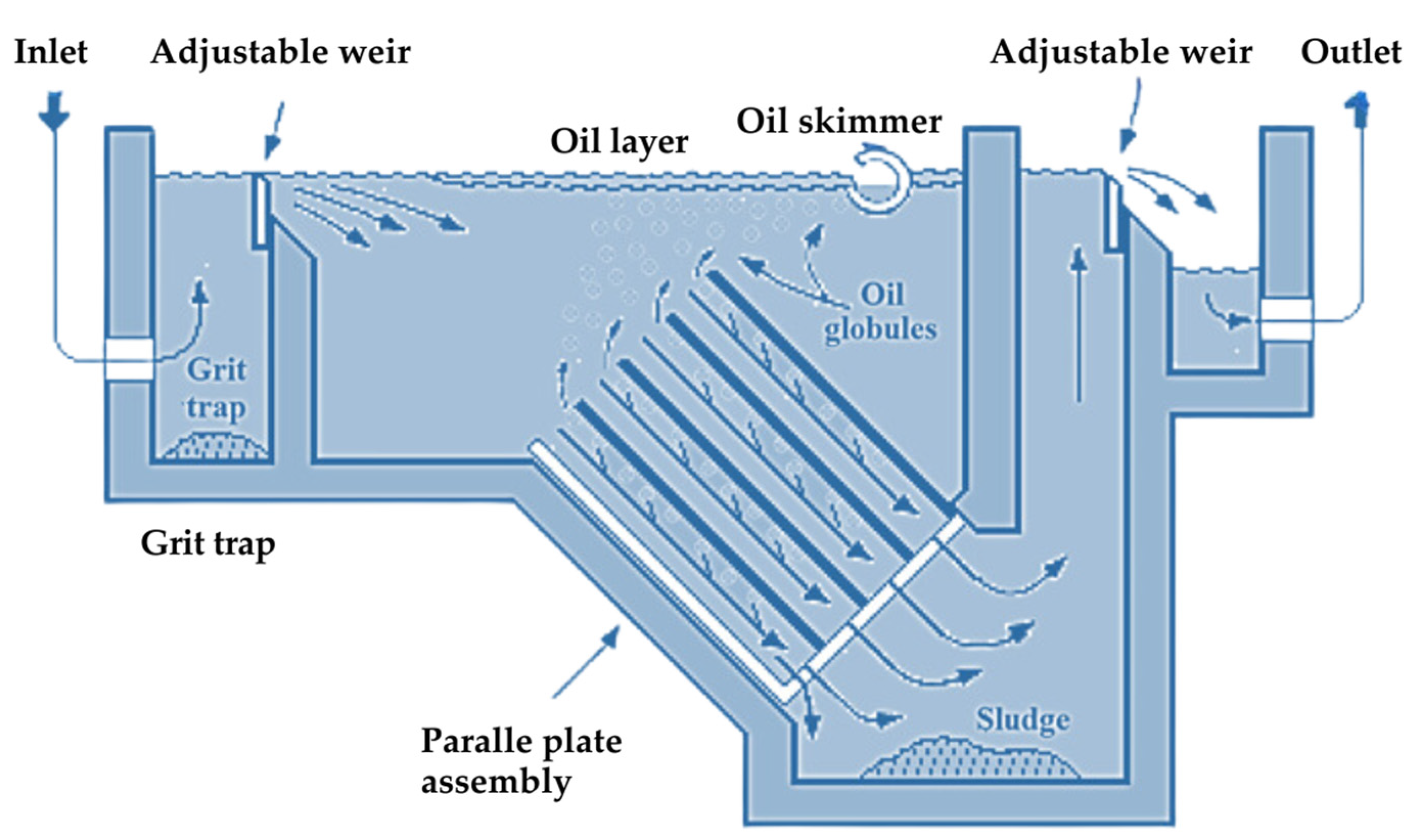Figure 1 illustrates a transverse sectional diagram of an API separator. It shows the separation process of oil and sludge from wastewater. The separator features an inlet and an outlet, each equipped with adjustable weirs, which help regulate the water flow. The grit trap collects heavier particles, while the parallel plate assembly enhances the separation of oil globules from the water. An oil skimmer is used to remove the separated oil layer from the surface, while sludge settles at the bottom for removal. The design helps in efficiently separating oil and solids from wastewater [16].

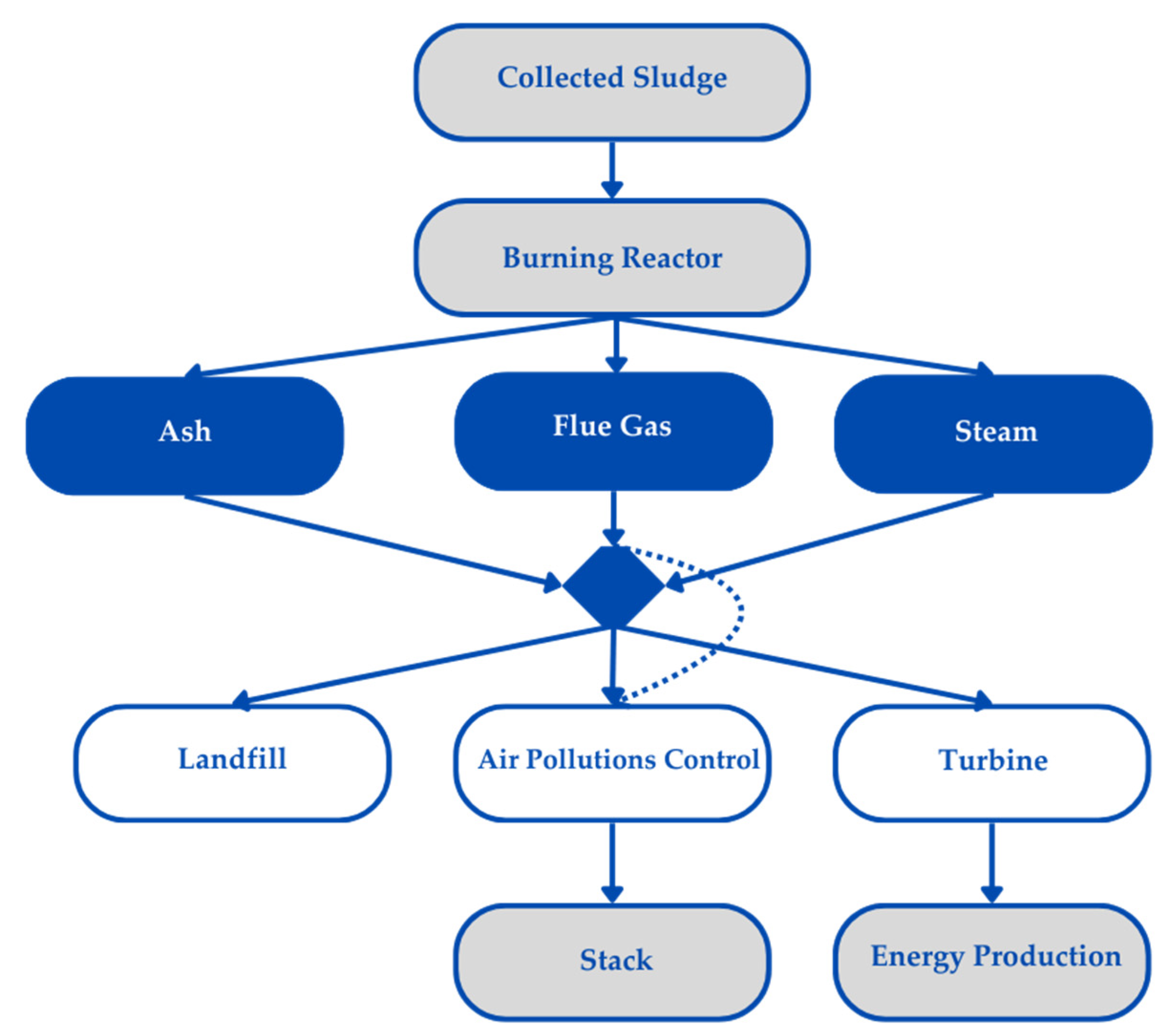
Figure 2 depicts a flowchart showing the waste-to-energy process involving sludge thermal recovery. The collected sludge is first directed into a burning reactor. The reactor produces ash, flue gas, and steam. The ash can be sent to a landfill, while the flue gas undergoes air pollution control before being released through a stack. The steam produced drives a turbine, which generates energy. This flowchart highlights the interconnected steps involved in converting sludge into usable energy while managing emissions and waste byproducts [14,15,16].

Within the domain of sludge thermal recovery research, various efforts focus on estimating calorific value. Thipkhunthod et al. in Bangkok, Thailand, approximated urban sewage sludge’s calorific value, incorporating ash in their models [17]. Shen et al. analyzed sludge components, developing models for predicting biomass calorific value [18]. Yin created regression models for biomass heating value prediction based on supplementary experiments [19]. Nhuchhen and Salam used analytic approaches to predict high-calorific-value sludge, enhancing prediction accuracy with an error function [20]. Wzorek explored sludge’s energy generation potential by combining it with high-value waste materials [21]. Rios et al. proposed an empirical formula correlating electricity output, methane gas calorific value, and organic matter in sewage treatment plants [22]. Ongen et al. assessed a fixed bed gasifier’s efficiency in extracting energy from chicken manure and oily sludge [23].

The management of hazardous solid waste, particularly petroleum oily sludge (POS), generated by the petroleum refinery industries has been a significant environmental challenge. Various studies have investigated the treatment and disposal approaches for POS to minimize its environmental impact. Singha and Deka [24] highlight that POS is the predominant solid waste produced during petroleum refining, containing complex mixtures of hydrocarbons, heavy metals, persistent organic compounds, and emulsions. For every 1000 tons of crude oil processed, around 5 tons of POS are generated. To mitigate environmental pollution, proper treatment technologies, such as freezing, thawing, centrifugation, and ultrasonic treatment, are employed before disposal. The waste management process involves reducing POS production, recovering oil, and finally disposing of the residual POS.

Dereli et al. [25] examine the incineration of gaseous and liquid hazardous wastes from used lubricating oil refineries. Their research focuses on achieving a zero-waste approach by combusting hazardous wastes along with natural gas. The study demonstrates the effectiveness of incineration at temperatures above 850 °C to achieve complete combustion and minimize harmful byproducts. The research further emphasizes the importance of material selection to withstand thermal stresses in the incinerator’s combustion chamber.

Wan et al. [26] explore the combustion characteristics of oily sludge in a fluidized bed reactor, focusing on emissions of nitrogen and sulfur pollutants and the migration of heavy metals like Cr, Ni, Cu, Zn, Cd, and Pb. The findings indicate that increasing temperatures and excess air ratios enhance emissions of nitrogen and sulfur pollutants. The study also reveals that a strong oxidizing atmosphere reduces heavy metal volatilization, with the migration and stability of heavy metals being influenced by their chemical forms in the ash.

Sahu et al. [27] discuss the complexities associated with the increasing production of petroleum refinery sludge, which contains hazardous compounds like cyanides and ammonia. They emphasize the potential of anaerobic digestion (AD) as a sustainable treatment option despite challenges related to sludge toxicity. The study outlines different AD strategies such as co-digestion and bioaugmentation, highlighting their effectiveness in mitigating sludge and recovering biogas.

Panda and Jain [28] focus on the detrimental environmental effects of untreated oil refinery effluents, which contain water-in-oil and oil-in-water emulsions as well as polyaromatic hydrocarbons. Given the growing energy demand, the study advocates for the integration of biorefineries into oil refineries to remediate sludge into valuable byproducts. Techniques like advanced oxidation processes, microwave-assisted wet air oxidation, and Fenton oxidation are discussed as viable treatment options to improve biodegradability and reduce the toxic effects of refinery sludge.

Collectively, these studies illustrate a range of treatment technologies and methodologies aimed at reducing the environmental impact of petroleum refinery sludge. They emphasize the need for effective treatment technologies, recovery of valuable byproducts, and sustainable waste management practices that align with the growing demand for cleaner and more efficient energy sources.

Mokhtar et al. [29] found a high HHV (higher heating value) (20.5 MJ/kg = 4900 kcal/kg) due to hydrocarbons, while the present study reports 3090 kcal/kg = 12.9 MJ/kg, linking sludge to waste-to-energy processes. Both highlight sludge composition, treatment challenges, and environmental concerns, promoting sustainable waste management strategies. The unification of our study emphasizes refining sludge characterization for optimized energy recovery and environmental sustainability. While Mokhtar et al. did not evaluate the effect of COD on the heat value of the sludge. The study [29] and Barneto et al. [30] both focus on oil refinery sludge characterization, emphasizing its energy potential and thermal behavior. While our study evaluates the calorific value (3090 kcal/kg = 12.9 MJ/kg) and sludge composition for waste-to-energy applications, Barneto et al. use thermogravimetric analysis to model sludge degradation and recovery potential. The unification lies in their shared goal of optimizing sludge utilization for sustainable energy and reducing environmental impact. However, the present study introduces a novel aspect by evaluating the effects of moisture percentage and COD variations across different storage zones, providing new insights into sludge characterization and management. Also, the research by Crelier and Dweck [31] addresses the impact of moisture content on oil sludge processing, particularly in thermal treatment methods. While Crelier and Dweck focus on how water content influences pyrolysis by affecting enthalpy and thermal balance, our study introduces new aspects by evaluating moisture percentage variations across different storage zones and their correlation with COD levels. Additionally, our research examines how these factors impact sludge properties before treatment, providing a broader understanding of sludge composition dynamics. The unification lies in understanding how moisture content alters sludge behavior during thermal processing, with our study offering novel insights into sludge variability before treatment, aiding in optimizing sludge management for sustainable energy recovery.

While existing literature often focuses on experimental methods in conventional wastewater treatment, the potential energy value of refinery sludge has been largely overlooked. This research addresses that gap by analyzing triangular interpolation plots of heat value profiles and performing a detailed case study on API sludge, aiming to uncover its energy potential. Refinery plant waste management and scheduling, a complex and often contentious issue in oil-rich countries, is a key focus of this study. This research seeks to determine the calorific value of accumulated sludge, develop statistical models to map sludge storage profiles, and provide practical managerial insights. The issue of refining plant waste scheduling has been underexplored by previous researchers, particularly in the context of optimizing waste-to-energy processes in countries with abundant oil resources. Figure A1 highlights the research novelties of this study: (1) spatial profiling of sludge to reveal energy heterogeneity across depths and zones; (2) development of predictive models using COD and moisture via RSM and regression; and (3) practical application of results to support energy recovery in refineries under circular economy principles.

By exploring the relationship between sludge incineration and energy generation, this study aims to turn a critical waste management problem into an opportunity for energy recovery. This research employs a case study of wastewater treatment practices at a petroleum refinery in Iran, aiming to provide a comprehensive assessment of sludge management. More specifically, the objectives of this study are as follows: (1) to determine the calorific value of sludge at various depths, (2) to establish transverse and longitudinal profiles of sludge storage using statistical modeling, and (3) to organize the available resources for effective presentation and storage of managerial insights. By addressing these objectives, this study contributes to a better understanding of how refinery waste can be managed to minimize environmental impact while maximizing energy recovery potential.

2. Materials and Methods

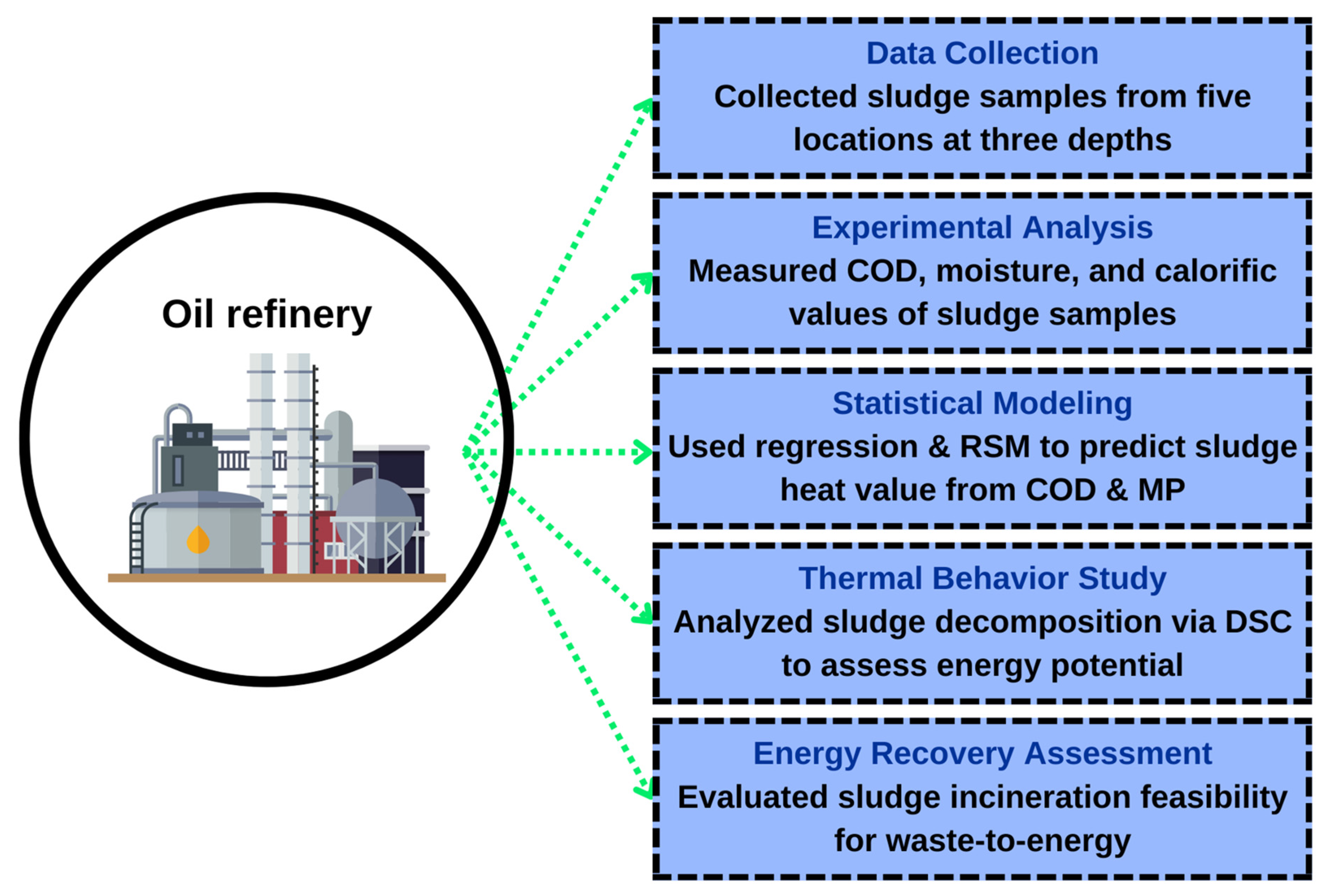
Figure 3 shows the research roadmap for sludge-to-energy evaluation in oil refineries. It includes data collection from five sites, experimental analysis of COD, moisture, and calorific values, statistical modeling via regression and RSM, thermal behavior study using DSC, and energy recovery assessment for incineration feasibility.

Fifteen sludge samples were systematically collected from five locations (P1–P5) within a 0.2 km diameter refinery sludge site during the summer of 2018 when ambient temperatures reached approximately 30 °C. Using a valve tube for sludge coring, samples were taken at three consistent depths—0.3 m, 0.6 m, and 0.9 m—resulting in a total of 15 sampling points. This depth-based sampling strategy ensured a comprehensive understanding of sludge characteristics across varying depths and spatial locations. The collected samples were then subjected to both experimental and numerical analysis. COD ranged from 27,000 to approximately 37,000 mg/kg, moisture content varied between 6% and 16%, and calorific values fluctuated from 2000 to 4000 kcal/kg. Analytical methods, including calorimetry, COD measurement, and DSC thermograms, confirmed a negative correlation between moisture content and energy potential. This carefully structured sampling and analysis process provides a robust foundation for assessing the environmental conditions and fuel potential of the sludge across the studied area. The reported ranges correspond to all samples collected from the various sampling points.

Samples were collected during the winter of 2021 over two consecutive days during regular operational hours at the refinery facility.

To understand and potentially mitigate the impact of petroleum oily sludge, this study began with data gathering. Sampling points were strategically chosen within the refinery process to collect sludge samples. Researchers gathered data on various sludge characteristics, ensuring a comprehensive understanding of its composition and properties. This step is critical, as it provides the foundational data for further analysis.

Following data collection, the sludge underwent experimental analysis aimed at breaking down its chemical structure. This stage is illustrated through a simplified chemical reaction where hydrocarbons react with oxygen, producing water, carbon compounds, and other byproducts. This reaction aims to reveal the sludge’s chemical composition and explore possible decomposition pathways. Through these experiments, this study evaluates the potential for treating or repurposing the sludge, moving closer to environmentally sustainable solutions.

Once experimental data were obtained, this study moved to the statistical and fundamental analysis stage. Here, statistical methods were applied to identify patterns and correlations within the data, offering deeper insights into the behavior and characteristics of the sludge under various conditions. This analysis not only strengthens the experimental findings but also enables researchers to refine their approach, creating a feedback loop that optimizes data gathering and experimental protocols. The roadmap includes two feedback loops. One loop connects experimental analysis to the data-gathering phase, allowing researchers to adjust sampling and refine experiments as new insights emerge. The other loop connects the statistical analysis back to data gathering, ensuring that each phase informs the next, leading to iterative improvements. Overall, this roadmap offers a clear, structured approach to understanding and managing petroleum oily sludge, aiming for environmentally friendly treatments and a deeper scientific understanding of this industrial byproduct.

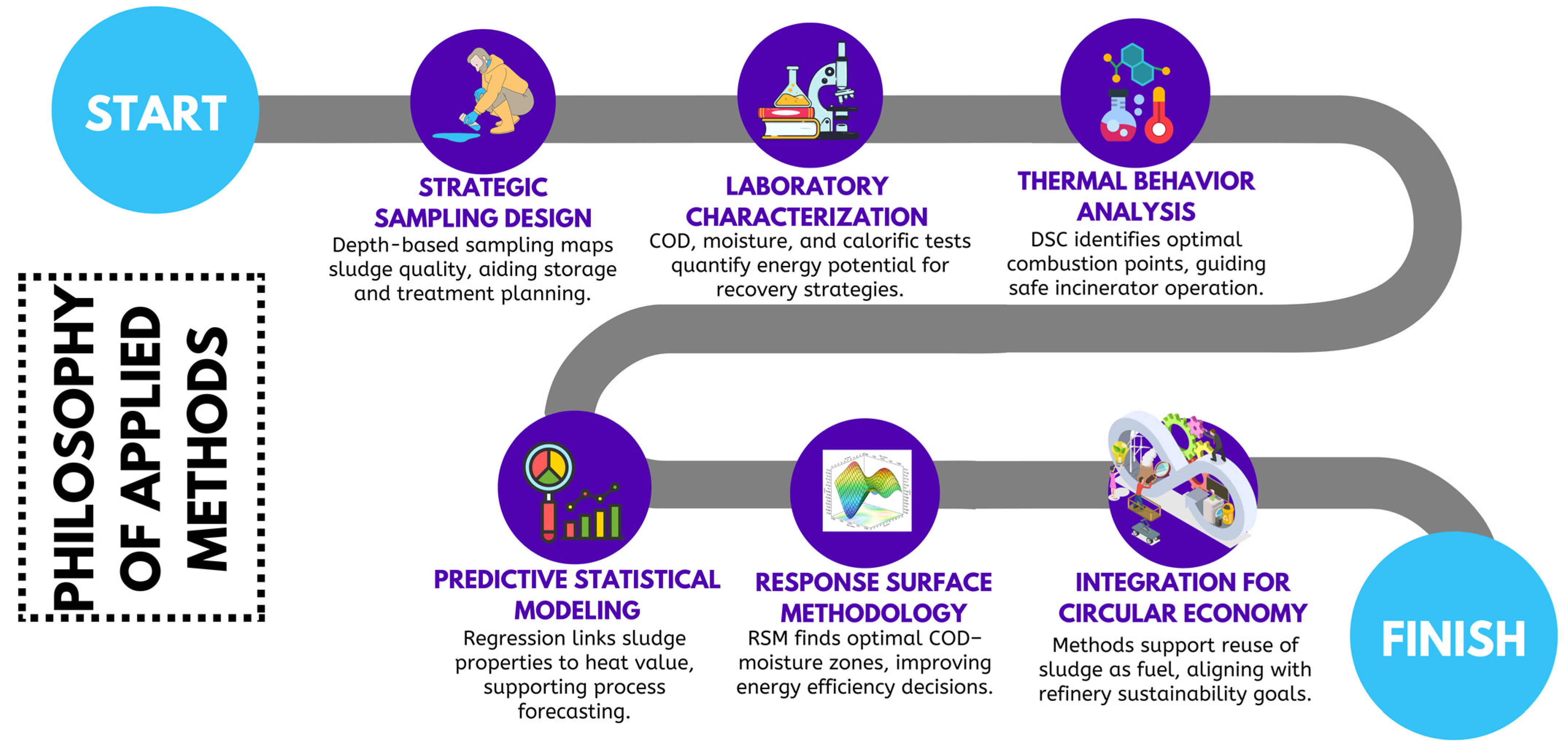
As illustrated in Figure A2, the multistage philosophy of applied methods begins with strategic sludge sampling and laboratory characterization, followed by thermal behavior analysis, predictive modeling, and RSM optimization, and concludes with integration into circular economy goals for refinery sustainability.

2.1. Case Study

The present examination centers on an oil refinery in Iran dedicated to processing gas for separation and purification purposes. The extraction of H2S gas, acting as a souring agent, takes place from the predominantly sweet gas produced by the refinery. The case study Gas Refinery is located 35 km from Sarakhs and 165 km from Mashhad, in the northeast of Khorasan province. The refinery currently consists of five gas processing units, three sulfur recovery units, two oil stabilization units, one sour water recovery unit, a wastewater treatment facility, and other auxiliary installations. The refinery’s wastewater treatment unit was constructed to recycle wastewater from the restaurant and sanitation facilities, as well as part of the industrial wastewater from sour water stabilization units, hydrocarbon tank drainage, and contact towers, with a treatment capacity of 500 m³/day of wastewater. However, another portion of the untreated wastewater is sent to evaporation ponds (as the target of this study) and ultimately to the surrounding lands of the refinery. Due to the high groundwater table in the area and the prolonged accumulation of untreated industrial wastewater, there is also a possibility of sewage infiltration from the Gonbadli village’s sanitary facilities and runoff from agricultural lands in the region. The effluent produced during the washing phase of the separation columns undergoes treatment within the API system. Resultant sludge contains notable volumes of petroleum, acidic chemicals, moisture, and organic substances. Figure 4 provides an illustrative representation of the essential organizational framework for sludge management at this refinery [32].

This study, conducted in summer 2018 with an average temperature of 31 °C, analyzed annual weather patterns, including cloud cover, precipitation, humidity, temperature comfort levels, and beach/pool suitability. Overcast conditions dominate in winter, transitioning to clear skies by July–August. Precipitation peaks at 2.54 cm in January, dropping to 0 cm in mid-summer, while humidity remains minimal year-round. Temperature comfort varies from cold in winter to sweltering in July–August. The beach/pool suitability score peaks at 8.7 in July, highlighting optimal conditions for outdoor activities. Overall, the climate shows distinct seasonal variations with dry, clear summers ideal for recreation [33].

2.2. Experimental Methods

Table 1. The tools and procedures used in this study.

Measurement Item	Devices	Procedures	Reference
Sludge’s heat value	PARR1266; calorimetry bomb; PreiserScientific (US)	ASTM-D294	[34]
COD measurement	Yatherm Scientific Company COD analyzer; (Indian)	Standard methods for the examination of water and wastewater	[35]
Moisture content detection	Schaller; Humimeter FS-4.1	Standard methods for the examination of water and wastewater	[36]

presents a summary of the equipment and procedures used in this study for the quantification of COD, the determination of sludge heat value, and moisture content analysis. The table provides details on the specific measurement items, the devices employed, the corresponding procedures, and relevant references for each analysis. For determining the sludge’s heat value, a PARR1266 calorimeter bomb from PreiserScientific (US) was utilized, following the ASTM-D294 standard [34]. For COD measurement, a COD analyzer from Yatherm Scientific Company (India) was used, examining both water and wastewater according to standard practices. Moisture content was detected using a Schaller Humimeter FS-4.1, with an examination method similar to that of COD, using Standard methods for the examination of water and wastewater. In a comparable fashion, the sampling technique employed a valve tube for sludge coring B10104 that was invented by Raven, an American corporation.

This detailed table ensures a comprehensive understanding of the tools and methodologies adopted in the experimental phase of the investigation, highlighting the rigorous approach taken to achieve accurate and reliable measurements. In this study, Differential scanning calorimetry (DSC) thermograms were obtained to characterize the refinery plant sludge, using the Perkin Elmer DSC Q100 instrument.

2.3. Large-Scale Heat Value Evaluation

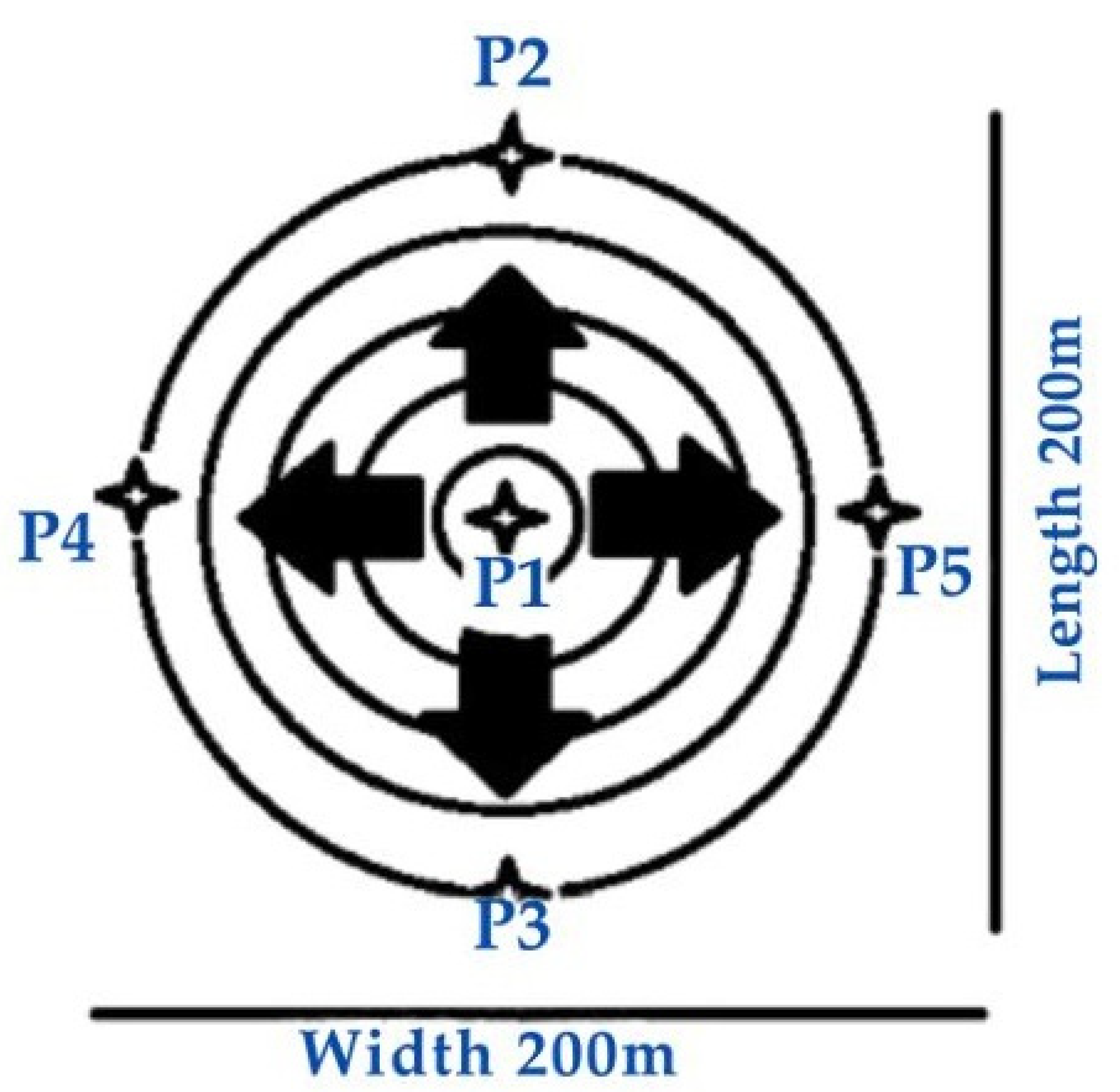
The sampling for this study was conducted from a circle measuring 0.2 km in diameter in order to assess the calorific value and conduct the sampling. The initial site of sludge accumulation during a span of five years is therefore situated at the midpoint of this ellipse. Although it is evident that the occupied property encompasses a greater area than this, for the purpose of determining the management criteria, only a 0.2 km diameter was assessed. Because under these conditions, the complete process may be examined and evaluated. The process of storing, as seen in Figure 5, is radial in nature, proceeding from the innermost to the outermost place. Consequently, the accumulation of sludge in the major areas persists for a longer duration than that on the margins.

In this study, the subsequent definitions are applicable to both transverse and longitudinal features. The structure of available sludge is solid with moisture percentage (semi-liquid), and therefore, with increasing depth of sample point, more force is applied for the process.

2.4. Classical Mathematical Modelling

In the present study, the experimental data—specifically moisture content and COD values—were initially correlated with the HHV using the Curve Fitting Tool (CF Tool) in MATLAB 2019. During the preliminary modeling phase, statistical indicators were employed to evaluate the performance of the developed model.

2.5. Sensitive Analysis and Optimization

To enable sensitivity analysis and extend the model, response surface methodology (RSM) was applied in the present research. Design Expert 7.0.0 software was utilized for modeling, sensitivity analysis, and ANOVA evaluation.

In the next step, after enhancing the model with detailed specifications of organic compounds, a comparative modeling approach was implemented using various machine learning algorithms, including Random Forest (RF), Gaussian Process Algorithm (GPA), Multilayer Perceptron (MLP), SMOreg, Lazy IBK (Instance-based k-nearest neighbor), Lazy LWL (Locally Weighted Learning), and Meta Bagging. All algorithms were executed using WEKA 3.9 software. The dataset was divided into 70% for training and 30% for testing in all machine learning evaluations.

2.6. Thermodynamics Analysis

The main objective of this study is to evaluate the thermodynamic performance of 15 sludge samples by estimating energy output, losses, and efficiency indicators. All computations and visualizations were performed using MATLAB 2019b. HHV, LHV (Lower Heating Value), and moisture percentage (MP) were used as input variables. Energy losses were calculated based on moisture evaporation loss Q_moisture = m_moisture × L, flue gas loss (10%), residue loss (5%), and unburned fraction Q_Unburned = HHV_total × (1 − η_comb)Q. Useful energy was derived as Q_useful = HHV_total × η_comb × η_turb, and efficiency metrics include thermal and exergy efficiency η_exergy = Q_useful/(HHV_total × (1 − T₀/T_comb)). A dashboard presents energy flow and efficiency comparisons across samples.

2.7. Economical Analysis

This study conducts a comprehensive economic assessment focused on Life Cycle Cost (LCC) analysis of a sludge-to-energy system, using MATLAB 2019b for all simulations. The analysis incorporates capital expenditure (EUR 900,000), annual operational costs (EUR 1M), and revenues based on 10,000 MWh/year energy sales at EUR 150/MWh with 2% annual growth. Key indicators such as net present value (NPV), internal rate of return (IRR), Benefit–Cost Ratio (BCR), and Payback Periods were calculated over a 25-year project lifetime with a 7% discount rate. The cash flows were adjusted for inflation (3%) and discounted to determine viability. Results are visualized via a dashboard highlighting costs, revenues, break-even, and key financial metrics.

3. Results and Discussion

The characterization of oily sludge (OS) by Jin et al. [37] highlights its complex composition and hazardous nature. OS is a mixture of water–oil emulsions and solid particles, typically consisting of approximately 30% oil, 40% water, and 30% solids. It contains heavy metals, organic pollutants, and bacteria, making it an environmental hazard if not properly managed. The proximate analysis shows a high volatile content (65.86 wt%) and low ash content (1.67 wt%), contributing to its potential for energy recovery. The ultimate analysis reveals a significant presence of carbon (60.39 wt%) and hydrogen (7.92 wt%), indicating a high organic matter content. Additionally, the sludge contains nitrogen (3.11 wt%), sulfur (0.25 wt%), and oxygen (26.66 wt%), which influence its chemical behavior and environmental impact. The sludge’s elemental composition includes metals such as Si, Al, Fe, Ca, Na, and Mg, with potential implications for processing and disposal.

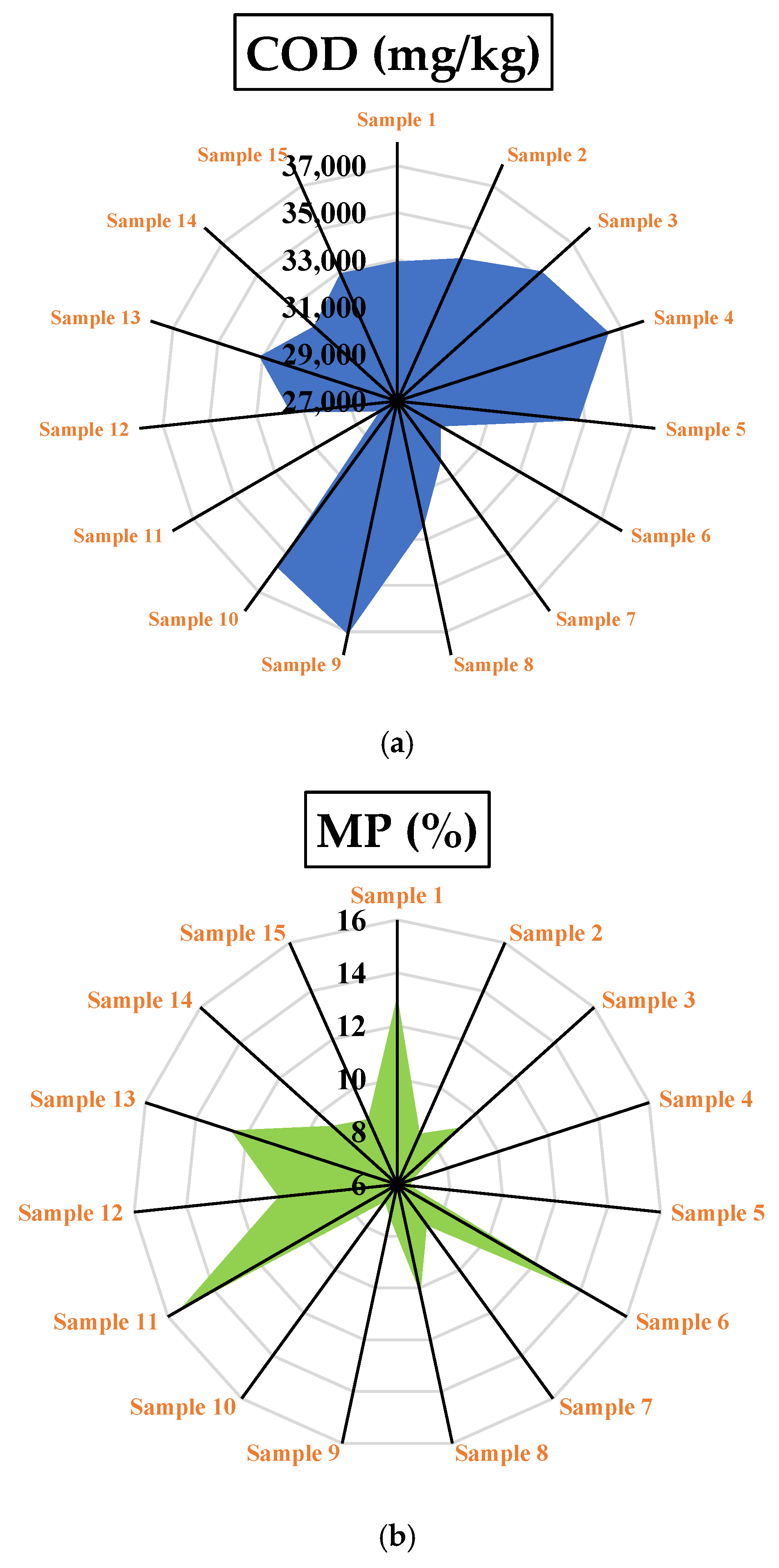
The results of diverse tests conducted on 15 samples are illustrated in Figure 6. As shown in Figure 6a, COD values of various samples vary from 27,100 to 37,050 mg/kg. Furthermore, the moisture percentage and sludge sample calorific value exhibit fluctuations of 6 to 16 percent (Figure 6b and heat value 2000 to less than 4000 kcal/kg, respectively (Figure 6c). In contrast to previous studies, the fluctuations in the moisture percent curve exhibit a nearly identical pattern to those observed in the COD and calorific value. Consequently, a direct association exists between the moisture content and the calorific value in relation to COD.

The HHV and LHV of the sludge (in MJ/kg) can be determined using Equation (1) [38]. In this equation, it is assumed that 1 kg of hydrogen generates approximately 9 kg of water (H₂O) during combustion. Therefore, the calculation is based on the assumption that the hydrogen content (H%) is equal to the moisture percentage divided by 9 (H% = Moisture% ÷ 9). The results of the LHV for the dried sludge are demonstrated in Figure 6d.

LHV = HHV − (9 × %H + %H₂O) × 2.44

(1)

Stehouwer et al. [39] conducted an extensive study on 7746 sludge samples from 177 publicly owned (wastewater) treatment works (POTWs) over a 20-year period, revealing notable seasonal and operational variability. The study found that inter-POTW variability was greater than intra-POTW variability, confirming that sludge properties are highly influenced by external factors such as wastewater composition and treatment efficiency. The coefficient of variation (CV) for NH₄-N exceeded 0.5, while the error margin for plant-available nitrogen application ranged from 0.39 to 1.09 of the intended amounts. This uncertainty suggests that seasonal fluctuations, along with treatment inefficiencies, can significantly impact nutrient concentrations. Additionally, trace element concentrations showed large variations, with lead (Pb) concentrations fluctuating within ±2 standard deviations, indicating a substantial degree of uncertainty in heavy metal distribution. The application uncertainty for trace elements, though large relative to single applications, was minimal in relation to cumulative loading limits, generally remaining below 0.01. Climate change exacerbates these variations by influencing precipitation patterns, temperature fluctuations, and industrial wastewater composition. Increased rainfall can lead to higher dilution of pollutants in sewage, altering sludge nutrient content, while extreme temperatures may affect microbial activity in treatment processes, impacting sludge stabilization. Furthermore, changing industrial discharge patterns due to climate adaptation strategies may lead to unpredictable shifts in sludge composition. The study’s findings emphasize the necessity for more frequent sampling and improved monitoring protocols to mitigate these uncertainties and ensure reliable sludge quality assessments [39].

MATLAB 2018b was used to simulate the function of implicit polynomials, with a second degree in the X-direction and a third degree in the Y-direction, for predicting accessible heat value (HV) energy based on the sludge’s moisture content in percent (MP) and COD, respectively, as shown in Figure 7. In the case of sludge samples with lower COD, their thermal energy levels decrease as relative humidity increases due to the ongoing anaerobic digestion process in deeper layers, as shown in the graph. Microbial activity results in a reduction in the organic load, and the anaerobic digestion occurs at a lower depth that promotes hydrolysis. Consequently, an increase in samples’ moisture content would lead to a rise in calorific value [20,21].

The regression model (Equation (2)) for predicting the HV of sludge based on the MP and COD values yielded promising results. The Sum of Squared Errors (SSE) was found to be 5.183 × 10⁴, indicating a moderate residual error when estimating HV from the input variables. The model achieved an R² value of 0.9881, suggesting that approximately 98.81% of the variance in HV can be explained by the MP and COD values, reflecting a high level of accuracy. The Root Mean Squared Error (RMSE) was 93.27, which quantifies the average deviation between observed and predicted values and is relatively low, showing good model fit. The adjusted R², at 0.9624, accounts for the number of predictors in the model and still indicates a strong explanatory power, confirming that the chosen variables are effective for predicting HV while avoiding overfitting. These statistical metrics demonstrate that the regression model provides a reliable and effective tool for predicting the heat value of sludge based on MP and COD.

HV = A00 + A10 MP + A01 COD + A20 MP² + A11 MP × COD + A02 COD² + A21 MP² × COD + A1² MP × COD² + A03 COD³

(2)

Ratios (with 95 percent confidence)

Regression Coefficients:

-

A00: (−2.067 × 10⁵, −7.254 × 10⁵, 2.868 × 10⁵)

-

A10: (9.326, −15.95, 35.66)

-

A01: (3.626 × 10⁴, −4.406 × 10⁴, 1.171 × 10⁵)

-

A20: (−0.0001034, −0.0004356, 0.0002053)

-

A11: (−1.376, −5.09, 2.385)

-

A02: (−1417.85, −3646.81, 647.19)

-

A21: (1.142 × 10⁻⁵, −2.878 × 10⁻⁵, 5.442 × 10⁻⁵)

-

A12: (0.02876, −0.02351, 0.08127)

-

A03: (17.25, 0.8327, 33.66)

Equation (2) established the suitability of a polynomial regression model. Subsequently, Equation (3) employed the response surface methodology (RSM) to derive a highly accurate quadratic equation. This approach was chosen because cubic models, which can exhibit varying ascending and descending trends, may not align with the underlying physics of the problem. In contrast, quadratic equations often provide a more consistent representation and are widely supported by existing studies [40,41,42]. Therefore, the quadratic model serves as the foundation for the analysis.

Through comprehensive regression model analysis utilizing historical data within the RSM framework, and employing Design Expert 7.0.0 software, a predictive quadratic regression model was developed, achieving an R² of 0.93 and a predicted R² of 0.71, as presented in Equation (3).

HV = +32,058.20274 − 1.39570 × COD − 1417.47530 × MP + 0.035335 × COD × MP + 1.73263 × 10⁻⁵ × COD² + 7.44860 × MP²

(3)

Table 2. The results of ANOVA analysis in the present study.

Source	F Value	p-Value (Prob > F)
Model	27.72974	<0.0001
A-COD	4.26082	0.0690
B-MP	2.859985	0.1251
AB	2.39887	0.1558
A2	1.343002	0.2763
B2	0.34175	0.5732

details the ANOVA results for the heat value concerning COD and MP across various samples, assessing both model significance and the contributions of individual factors. The model demonstrates high significance (p < 0.0001), underscoring a robust correlation between the predictors and the response variable. The linear terms, A-COD (p = 0.0690) and B-MP (p = 0.1251), exhibit moderate significance, suggesting their notable impact on the heat value. In contrast, the interaction term (AB) and quadratic terms (A², B²) display lower significance levels, indicating minimal interactive or nonlinear effects between COD and MP on the heat value.

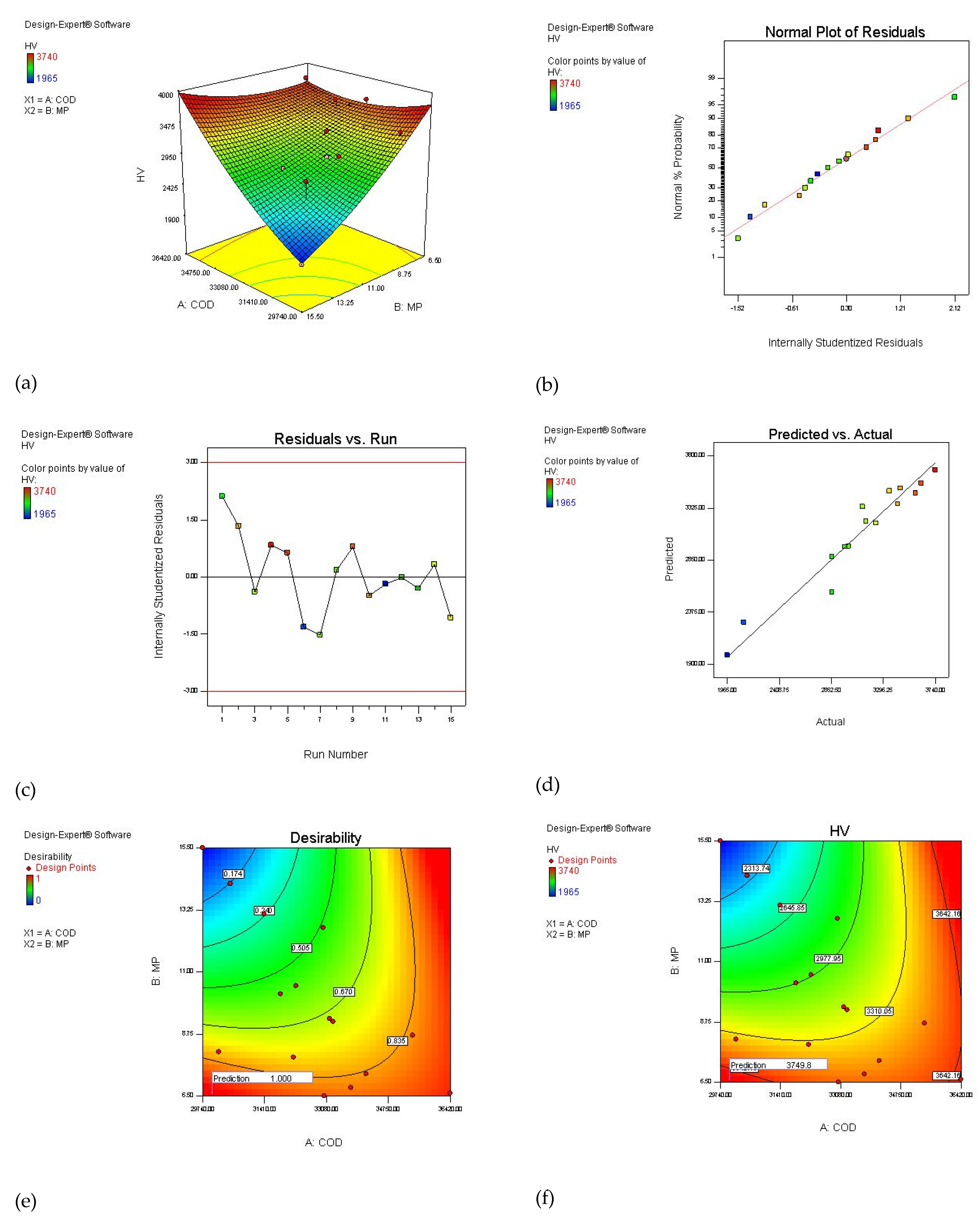
Figure 8a illustrates the sensitivity analysis of the model, displaying the response surface plot of HV as a function of COD and MP. The three-dimensional representation provides insights into the interactive effects of these parameters, where HV exhibits a nonlinear trend. The visualization suggests that increasing MP leads to a significant rise in HV, while COD demonstrates a more complex impact, indicating the necessity of optimizing both parameters for enhanced performance.

Figure 8b presents the normal plot of residuals, evaluating the normality distribution of the dataset. The points align closely with the diagonal reference line, suggesting that the residuals are approximately normally distributed. This indicates that the model’s assumptions hold true, ensuring reliable predictions and statistical validity.

Figure 8c illustrates the residuals versus run number, providing insight into the error distribution throughout the experiments. The plot shows that the residuals are randomly scattered without any discernible trend, confirming that there is no systematic error in the experimental setup. The absence of a clear pattern suggests that the model effectively captures the variability in the data without significant bias.

Figure 8d compares the predicted HV values with the actual experimental results, demonstrating the accuracy of the model’s predictions. The data closely align with the 45-degree diagonal line, indicating a strong correlation between the predicted and observed values. The minimal deviation suggests that the model provides a reliable estimation of HV under different experimental conditions.

Figure 8e depicts the desirability function, highlighting the most favorable regions for achieving optimal conditions based on the model’s predictions. The contour plot identifies specific areas where the desirability index is maximized, guiding the selection of optimal COD and MP values. The design points provide additional verification of the model’s applicability in real-world scenarios.

Figure 8f illustrates the contour plot of HV, emphasizing the optimal maximum achievable points. The heatmap representation indicates regions where HV reaches its peak, guiding parameter selection for enhanced performance. The optimal conditions identified in this plot align with the sensitivity analysis, reinforcing the model’s predictive capability in determining the highest HV values.

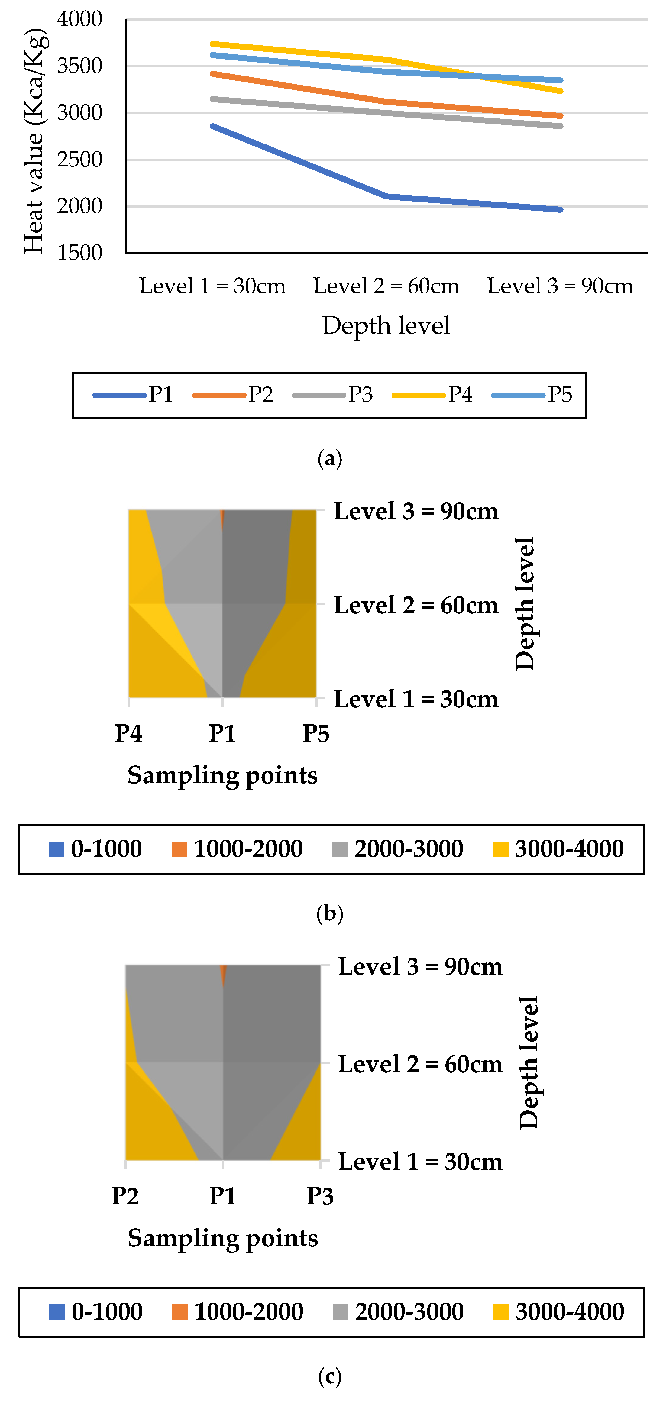
As discussed earlier, the calorific value decreases with increasing sampling depth due to the in-depth progression of anaerobic digestion of organic compounds, as illustrated in Figure 9a. The longitudinal and transverse profiles, shown in Figure 9b,c, reveal that the lowest heat value is observed at point P1, corresponding to the oldest sludge storage location. This trend is likely attributable to the metabolic activities of anaerobic bacteria, which play a critical role in the breakdown of organic matter. Over a five-year period [34], these metabolic processes have had sufficient time to complete, further contributing to the observed reduction in calorific value.

This refinery processes approximately 4000 tons of accumulated sludge with an average calorific value of 3090 kcal/kg, enabling the generation of a substantial amount of energy over its estimated five-year operational period (around 12,400 GCal). However, operators must be well versed in managing air pollution and ash byproducts resulting from combustion and adhere to critical management principles to mitigate environmental impacts [36].

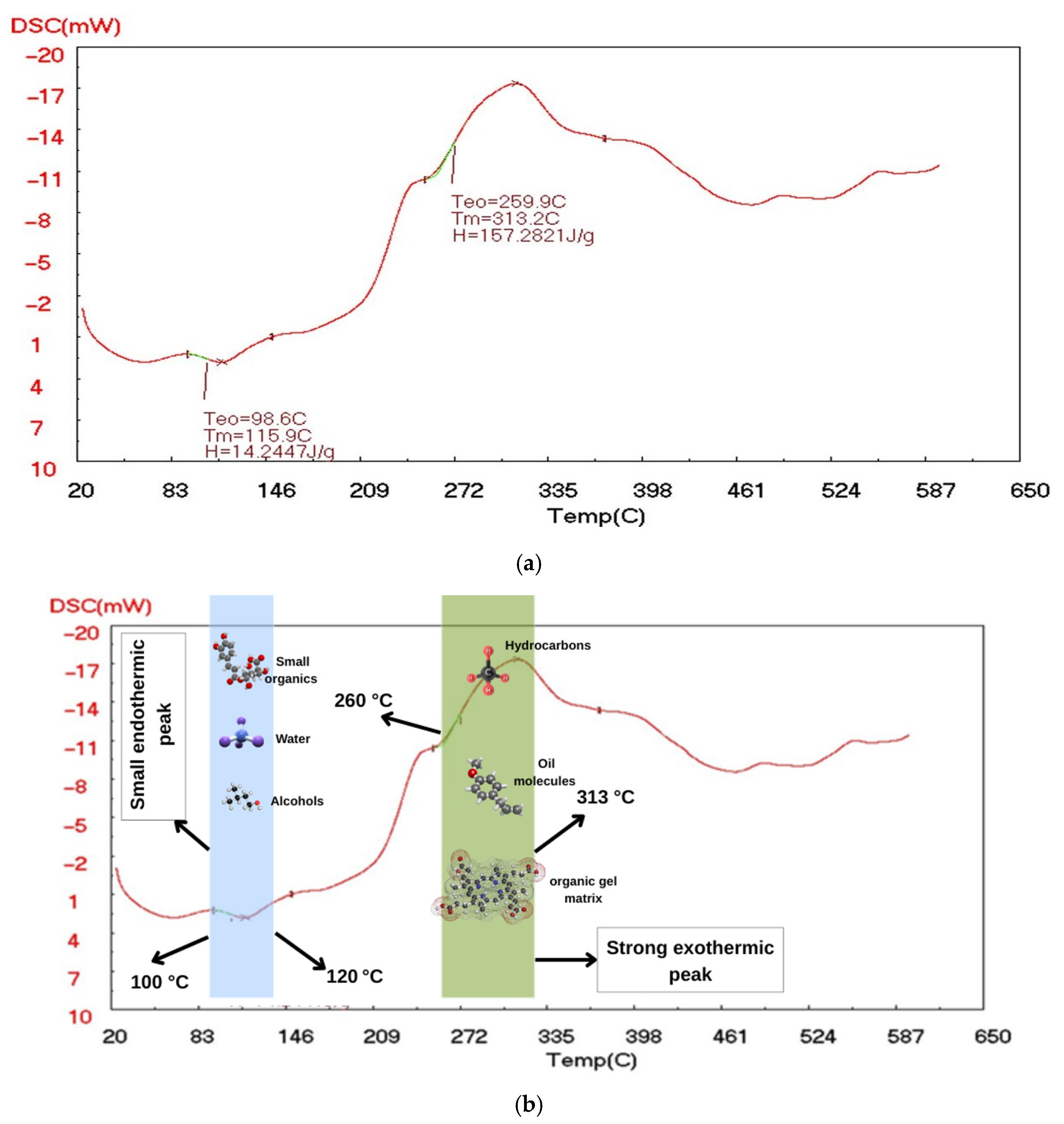
Figure 10a illustrates the Differential scanning calorimetry (DSC) curve of refinery sludge, offering insights into the thermal transitions of the material. DSC is a versatile analytical tool that evaluates heat flow associated with physical and chemical transitions, such as melting, decomposition, and phase changes.

The DSC curve reveals two significant endothermic peaks and two exothermic transitions. The first endothermic peak occurs at 115.9 °C, with an enthalpy change of 14.2447 J/g. This is likely associated with the evaporation of water or light volatiles within the sludge. The second endothermic peak is observed at 313.2 °C, with a higher enthalpy value of 157.2821 J/g, suggesting the decomposition or melting of high-molecular-weight organic materials, such as hydrocarbons typically found in refinery sludges. The substantial energy requirement for this transition reflects the complexity of these organic compounds.

Exothermic transitions occur at (1) 98.6 °C, which may correspond to the oxidation of reactive components like light volatiles or easily oxidizable organics, and (2) 259.9 °C, indicating more substantial oxidation reactions or structural rearrangements, potentially involving reactive hydrocarbons or metal compounds.

These thermal transitions across a wide temperature range highlight the heterogeneous nature of refinery sludge. It consists of diverse components, including water, light hydrocarbons, heavy organic compounds, and potentially metals, each exhibiting distinct thermal behaviors. The varying thermal stability observed in Figure 10 reflects the intricate composition of refinery sludge, with each component undergoing unique transformations at different temperatures.

From a thermodynamic perspective, the significant energy requirement at 313.2 °C indicates a high input is necessary to process the sludge beyond this point. This has practical implications for thermal treatment processes, e.g., incineration or pyrolysis, where understanding these transitions helps optimize temperature settings and energy use. Moreover, the combination of endothermic and exothermic behaviors suggests opportunities for energy recovery during sludge processing, depending on the specific components treated.

Figure 10b illustrates the DSC curve of oily sludge, highlighting two main thermal events. A small endothermic peak appears around 100–120 °C, attributed to the evaporation of water, alcohol, and light organics. A strong exothermic peak occurs between 260 and 313 °C, with a maximum at 313 °C, corresponding to the oxidation of hydrocarbons and breakdown of the organic gel matrix. This thermal behavior reflects the stepwise decomposition and energy release of sludge components, consistent with its high HHV.

Our study on sludge incineration for energy recovery from industrial wastewater treatment demonstrates notable parallels and contrasts with the works of Dereli et al. [25], Wan et al. [26], and Ji et al. [39], which focused on hazardous waste incineration and pyrolysis. A common theme across all studies is the emphasis on maintaining high temperatures to enhance waste decomposition and minimize harmful byproducts.

Wan et al. [26] focused on oily sludge combustion in a fluidized bed reactor at temperatures between 850 and 1050 °C, analyzing emissions of nitrogen and sulfur compounds as well as heavy metal migration. They found that higher temperatures and increased air ratios elevated NOx and SO₂ emissions while also influencing the retention of heavy metals in bottom ash. Similarly, our study emphasized the importance of controlling combustion conditions to reduce harmful emissions. The findings of Wan et al. on heavy metal migration and stability are directly relevant to the complex composition of our sludge. In our study, by analyzing the moisture percentage, the correlation between the HHV and Lower Heating Value (LHV) was scrutinized. Our findings highlight that an increase in MP% leads to a significant reduction in LHV due to the additional energy required to evaporate water before combustion can proceed efficiently. This energy loss reduces the net heat output and lowers combustion efficiency. Moreover, a higher moisture content results in lower flame temperatures, incomplete combustion, and increased latent heat losses in the flue gas, further diminishing the effective energy yield.

Ji et al. [39] explored the pyrolysis of oily sludge as a sustainable alternative to incineration, using a life cycle assessment (LCA) to evaluate environmental impacts. Their results indicated that pyrolysis has a lower global warming potential (GWP) compared to incineration. Major contributors to GWP included processes such as flue gas purification and hot washing, while recycling pyrolytic oil and residues mitigated adverse effects. They also emphasized decarbonization strategies such as employing green electricity and co-pyrolysis. While our study focused on energy recovery through incineration and did not incorporate an LCA, Ji et al.’s findings highlight the environmental benefits of alternative thermal treatments. This insight complements our efforts to optimize sludge management for energy recovery and suggests future exploration of sustainable alternatives such as pyrolysis.

In terms of methodology, all studies utilized numerical analysis to refine waste treatment processes. Dereli et al. used simulations to enhance combustion, Wan et al. employed BCR sequential extraction to study heavy metal migration, and Ji et al. relied on LCA for environmental impact assessments. In our study, we applied quadratic regression to predict heat value based on sludge properties such as moisture content and COD, achieving an R² value of 0.93. This approach effectively captured the relationship between sludge characteristics and calorific value, contributing to improved efficiency in sludge incineration.

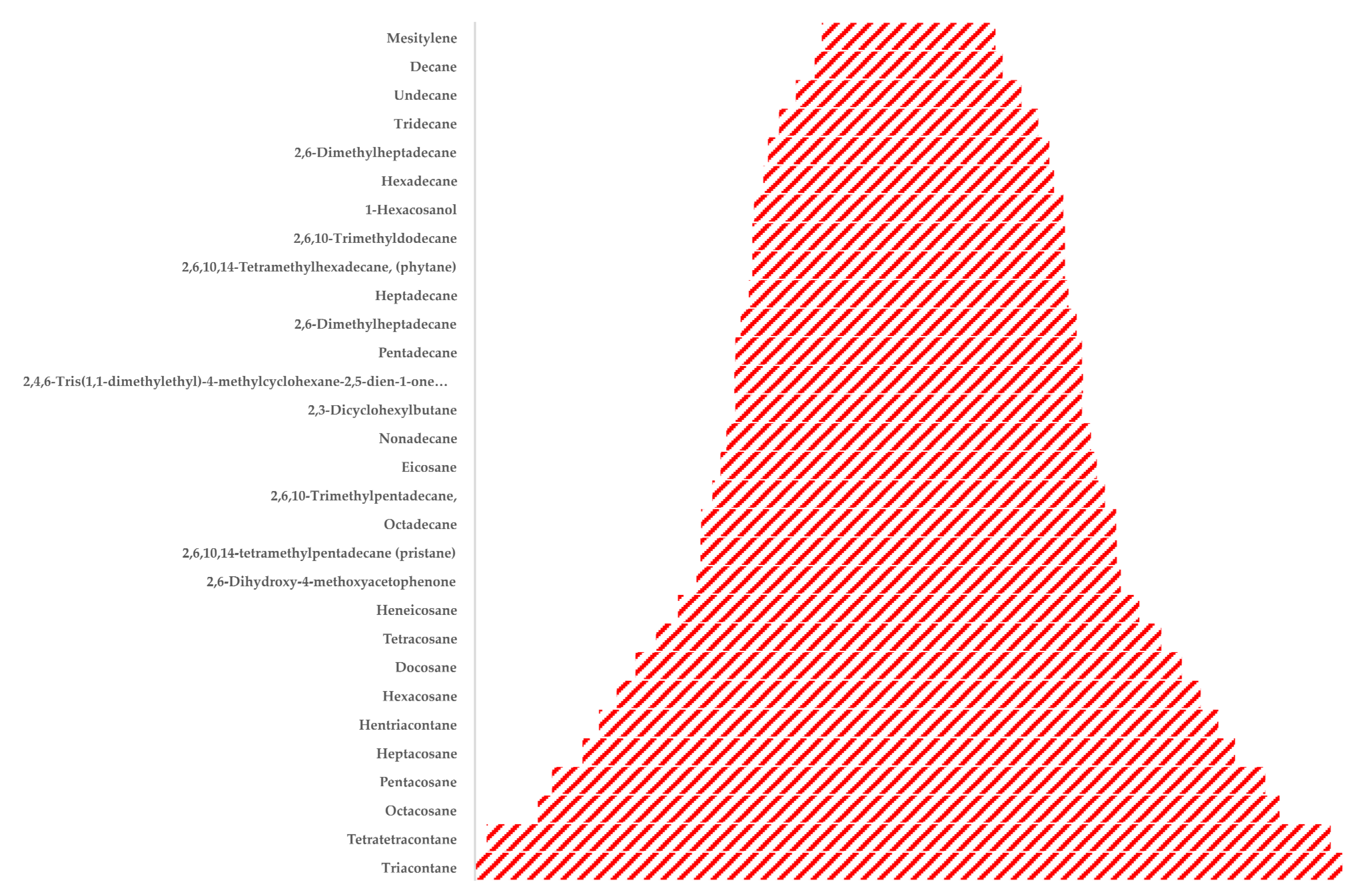
The Gas Chromatography (GC) analysis of petroleum sludge in the research of Jerez et al. (2021) [41], as presented in Figure 11, reveals a comprehensive distribution of hydrocarbon compounds with varying retention times (r.t). The detected compounds range from light hydrocarbons such as mesitylene (6.87 min) to heavy hydrocarbons including triacontane (34.307 min). The chromatographic profile highlights the presence of alkanes, branched alkanes, and oxygenated compounds, reflecting the complex composition of petroleum sludge. In the lower retention time range, volatile hydrocarbons, such as mesitylene (6.87 min), decane (7.44 min), and undecane (8.92 min), are observed, indicating lighter fractions within the sludge. Moving to the mid-range, compounds such as heptadecane (12.642 min) and nonadecane (14.423 min) appear, representing longer-chain alkanes with moderate volatility. The presence of branched hydrocarbons like 2,6,10-trimethylpentadecane (15.528 min) and pristane (16.47 min) suggests the existence of isoprenoid structures commonly found in petroleum products. The high retention time region is dominated by long-chain hydrocarbons, including docosane (21.603 min), hentriacontane (24.496 min), and octacosane (29.335 min), which are indicative of waxy and heavy petroleum fractions. The detection of tetratetracontane (33.383 min) and triacontane (34.307 min) further confirms the presence of high-molecular-weight hydrocarbons, emphasizing the sludge’s complex and persistent nature. The numerical distribution of retention times confirms the presence of a diverse range of hydrocarbons, spanning from light, volatile fractions to heavy, long-chain alkanes. This characterization provides insight into the sludge’s chemical composition, which is crucial for its further processing, treatment, or utilization in energy recovery applications.

The study by Huang et al. [43] presents a comprehensive quantitative assessment of the environmental and economic benefits of sludge-to-energy incineration approaches. The research evaluates four sludge treatment routes—co-incineration in coal power plants (CIN), mono-incineration (IN), anaerobic digestion (AD), and pyrolysis (PY)—using an integrated methodology combining life cycle assessment (LCA), Techno-Economic Analysis (TEA), and the Analytic Hierarchy Process (AHP)-Entropy method. The study finds that CIN exhibits the best overall performance, followed by PY, while IN ranks the lowest due to its high costs and significant environmental burden. From an environmental perspective, the study assesses multiple impact categories. In terms of global warming potential (GWP), CIN demonstrates the lowest emissions at 177.75 kg CO₂-eq per ton of dry sludge (t DS), while IN has the highest emissions at 689.45 kg CO₂-eq/t DS due to its high fossil fuel consumption. Heavy metal contamination is another critical factor, with IN exhibiting the highest human toxicity potential (HTP), primarily due to fly ash disposal, whereas AD has elevated freshwater (FEP) and terrestrial ecotoxicity potential (TEP) due to heavy metal leaching during digestate land application. Fossil fuel depletion (ADP-F) is most severe for IN, while CIN and AD perform well due to energy recovery through electricity generation and biogas substitution. Acidification and eutrophication potential are highest for AD, primarily because of nutrient leaching from digestate land application. While photochemical oxidation and ozone depletion potential are comparatively minor, IN exhibits the highest photochemical ozone creation potential (POCP) due to NOx emissions. The techno-economic assessment highlights notable differences in financial viability across the four treatment routes. CIN, PY, and AD exhibit relatively high net present values (NPV) at 141.2, 219.2, and 254.1 CNY/t DS, respectively, whereas IN has a significantly lower NPV of 33.1 CNY/t DS, making it economically less attractive. The dynamic payback period (DPP) further supports the superiority of CIN, with the shortest investment recovery time of 5.36 years, compared to 12.83 years for IN. In terms of the internal rate of return (IRR), all routes surpass the 8% economic viability benchmark, with PY leading at 16.3%, followed by CIN (16.2%) and AD (14.93%). IN, however, barely remains feasible at 8.87%, further reinforcing its economic disadvantage. Sensitivity analyses reveal that both organic content and sludge reception fees significantly influence the environmental and economic performance of all four routes. Higher volatile solids (VSs) content, increasing from 40% to 70%, improves economic returns by enhancing energy recovery. Similarly, sludge reception fee variations impact the financial feasibility of treatment routes, with IN being the most vulnerable to revenue fluctuations. These findings suggest that policies promoting higher sludge organic content and stable financial incentives can enhance the economic sustainability of sludge-to-energy conversion.

According to Nkuna et al. [44], the cost–benefit analysis of sludge incineration reveals that the overall feasibility depends significantly on the scale of the plant, operational efficiency, and energy recovery potential. Large-scale incineration plants with a capacity of 35,000 Mg ds/a require an investment of EUR 35 million, with annual operational costs of EUR 5.5 million, translating to a treatment cost of EUR 157 per Mg ds. Medium-scale plants (4000 Mg ds/a) demand an investment of EUR 12 million and annual operational costs of EUR 1 million, leading to higher treatment costs of EUR 487 per Mg ds. Small-scale plants (2000 Mg ds/a) are the least cost-effective, with an investment of EUR 16 million, annual operational costs of EUR 1 million, and treatment costs reaching EUR 510 per Mg ds. These data suggest that larger plants benefit from economies of scale, making them more viable for long-term operation. From an economic feasibility standpoint, energy recovery through gasification presents a compelling case for investment. Over a 25-year period, gasification is projected to yield a profit ranging from 4.3% to 7.5%, with a net present value (NPV) of EUR 1,801,700 after nine years. The internal rate of return (IRR) is estimated at 2.55%, with a payback period of approximately six years. The energy output from gasification is substantial, with an annual electricity generation of 427.78 MWh, of which 270.4 MWh can be supplied to the grid, contributing to an annual energy profitability of EUR 70,947. However, the economic feasibility is highly dependent on drying costs, H₂ generation from synthesis gas, and municipal solid waste (MSW) processing, all of which influence the financial sustainability of the project. Environmental considerations play a crucial role in determining the viability of sludge incineration, particularly in managing pollutant emissions and complying with regulatory standards. The combustion of wastewater sludge (WWS) produces nitrogen oxides (NOX) in the range of 1250–2250 ppm, which necessitates advanced emission control measures. Studies show that incineration significantly reduces toxic hazards, decreasing pollutant levels from 777.07 in raw WWS to 64.55 in slag and 288.72 in fly ash. However, gas cleaning and ash disposal introduce additional costs, making regulatory compliance a significant financial burden. Technologies such as filtration devices, fabric filters, and packed-bed scrubbers have been implemented to mitigate emissions of NOX, SO₂, and HF, further influencing the operational costs of sludge incineration. The efficiency of energy recovery varies depending on the conversion technology used. Fluidized Bed Combustion (FBC) has proven to be highly effective, achieving an energy recovery efficiency of approximately 80%, with electricity generation accounting for 20% of the total energy output. Furthermore, integrated sludge and MSW incineration have been identified as the most profitable approach, particularly when incorporating coal co-incineration, which results in a turnover profit of 89.74%. This highlights the potential for optimizing incineration processes by integrating multiple waste streams to enhance overall energy recovery and cost efficiency. Investment and operational costs are critical determinants of the economic sustainability of sludge incineration. The drying process alone requires a capital investment of EUR 150,000, with annual maintenance costs of EUR 7500. Gasification technology demands an even higher investment, with a gasifier purchase price of EUR 140,431.2 and annual maintenance costs of EUR 7021.56. The total venture capital for an integrated energy recovery unit is estimated at EUR 295,431.2, with an annual maintenance cost of EUR 36,371.56. These outcomes underscore the need for cost-effective energy recovery strategies to justify the high capital expenditure associated with sludge incineration [44].

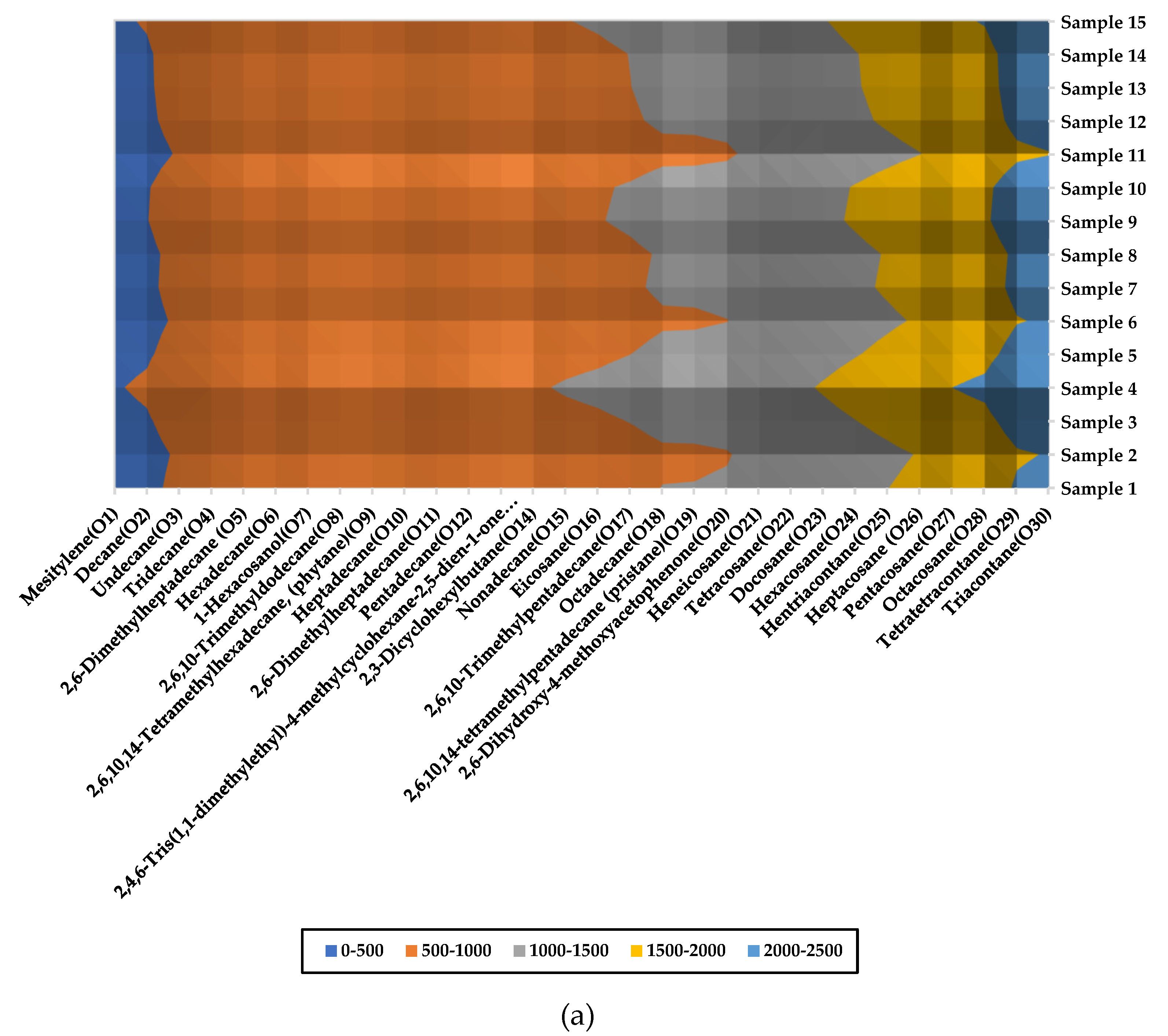
In the next step, based on the GC output reported by Jerez et al. [41], the percentage of each compound was calculated. Subsequently, the mass concentration (mg/kg) of each compound was determined using the COD values, as illustrated in Figure 12a. Accordingly, the model inputs included moisture content, COD values, and 30 features corresponding to different organic compounds (O1, O2, …, O30), while the HHV was considered as the output variable.

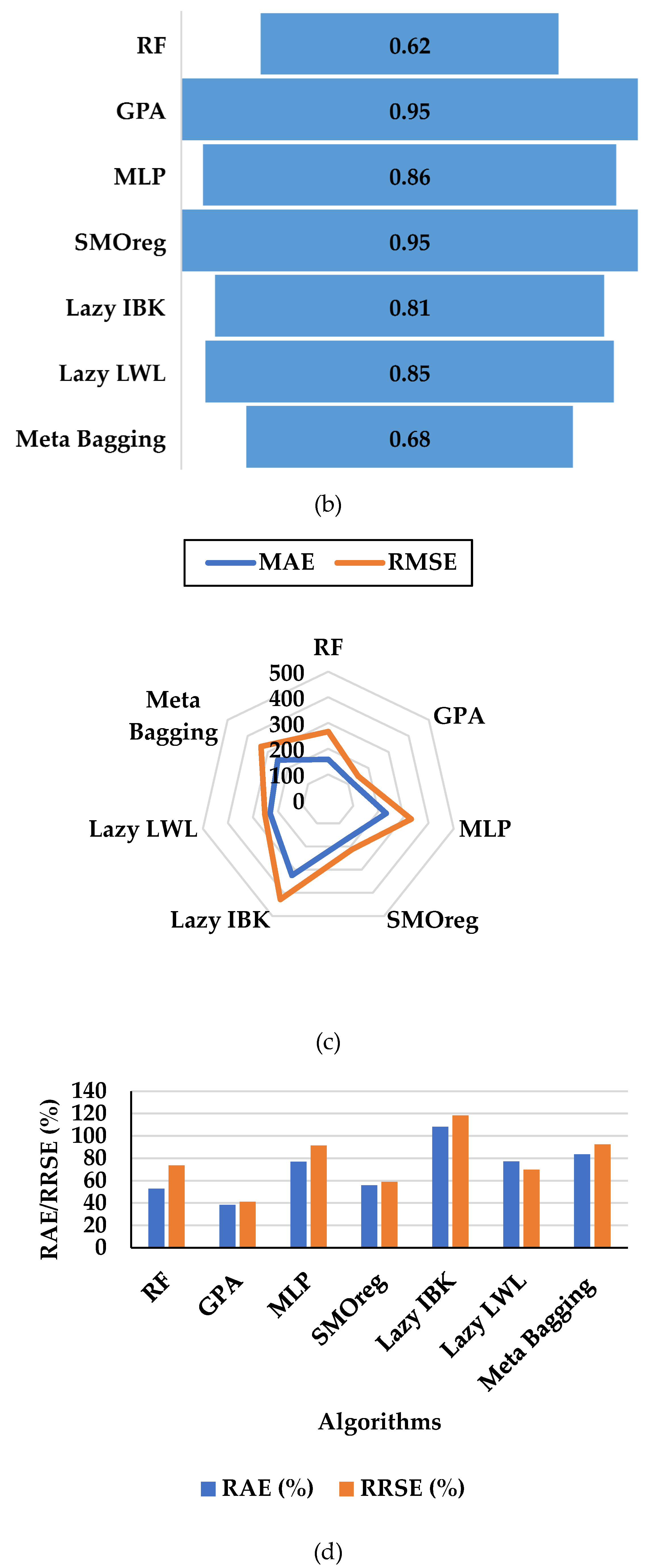
Figure 12b presents the correlation coefficients (CC: R values) obtained from different regression algorithms implemented in WEKA. The GPA and SMOreg yielded the highest predictive correlations, both achieving R = 0.95, reflecting strong agreement between the predicted and actual HHV values. This was followed by MLP (R = 0.86), Lazy LWL (R = 0.85), and Lazy IBK (R = 0.81). Random Forest and Meta Bagging demonstrated lower performance with R values of 0.62 and 0.68, respectively. Figure 12c compares the Mean Absolute Error (MAE) and Root Mean Square Error (RMSE) using a radar plot. GPA and SMOreg recorded the lowest MAE and RMSE values, confirming their high accuracy and reliability. In contrast, Lazy IBK and Lazy LWL presented noticeably higher errors, implying weaker generalization capability. Meta Bagging and Random Forest fell in the mid-range. Figure 12d shows the Relative Absolute Error (RAE) and Root Relative Squared Error (RRSE) for each algorithm. GPA and SMOreg again outperformed the others with the lowest RAE and RRSE percentages. The Lazy learning algorithms (IBK and LWL) and Meta Bagging exhibited significantly higher relative errors, reinforcing their comparatively lower accuracy.

GPA and SMOreg showed the best performance with R = 0.95 and the lowest MAE, RMSE, RAE, and RRSE, indicating high accuracy. MLP and Lazy LWL followed, while Random Forest, Meta Bagging, and Lazy IBK showed weaker predictive capability. Finally, all outcomes of different algorithms in WEKA 3.9 software are mentioned in Equations (A1)–(A7).

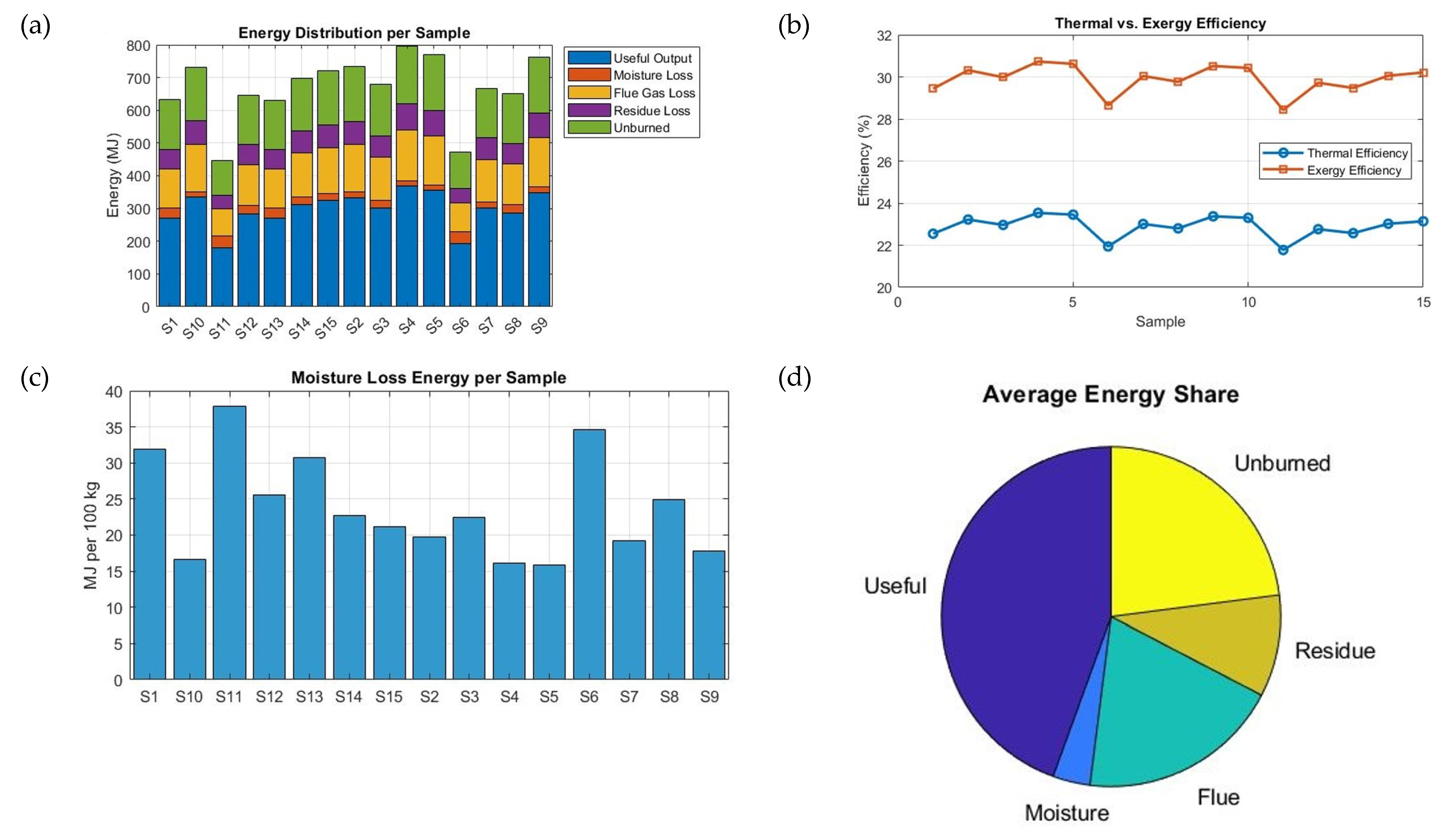
Figure 13 offers a comprehensive thermodynamic dashboard that illustrates the energy distribution, efficiency metrics, and loss components associated with the combustion of 15 distinct sludge samples. Each subplot of Figure 13a–d highlights a key dimension of performance, with data normalized for a batch mass of 100 kg to ensure comparability.

Figure 13a decomposes the total HHV energy input of each sludge sample into five categories: useful output, moisture loss, flue gas loss, residue loss, and unburned energy. The total energy input per sample ranges from approximately 822 MJ (Sample S11) to 1565 MJ (Sample S4), reflecting variability in HHV values across the samples. For instance, Sample S4, with the highest HHV (15.648 MJ/kg), produces the greatest amount of useful energy at approximately 368.29 MJ due to favorable combustion and turbine efficiencies. In contrast, Sample S11, with the lowest HHV (8.221 MJ/kg) and the highest moisture content (15.5%), delivers only about 179 MJ of useful energy, severely impacted by both moisture losses (approximately 37.82 MJ) and reduced combustion efficiency (around 0.869). Unburned energy represents a significant portion of the losses across all samples, driven by the inverse relation between combustion efficiency and moisture percentage. Flue and residue losses, held constant at 10% and 5% of HHV, respectively, also contribute meaningfully.

Figure 13b compares the thermal efficiency and exergy efficiency for each sample. Thermal efficiency, defined as the ratio of useful energy to total HHV, ranges narrowly between 21.7% and 23.5% across the samples. The highest thermal efficiency is observed in Sample S4 (23.5%), aligning with its high HHV and low moisture content. Sample S11 again shows the lowest performance with approximately 21.7% thermal efficiency due to high moisture penalties and low turbine efficiency. In contrast, exergy efficiency, which accounts for the quality of energy and ambient-to-combustion temperature gradients, consistently trends higher, falling between 28.42% and 30.7%. The peak exergy efficiency is again recorded for Sample S4, reaching 30.7%, while S11 dips to the lowest at 28.42%, reinforcing the energy quality loss due to moisture and low-grade heat sources. According to Figure 13c, moisture energy loss, computed using each sample’s moisture percentage and the latent heat of vaporization (2.44 MJ/kg), shows a clear and substantial variation. The highest moisture energy loss occurs in Sample S11 (37.82 MJ), directly attributable to its 15.5% moisture content. Figure 13d summarizes the average distribution of energy across all samples. On average, useful output accounts for approximately 30% of the total input energy, making it the largest single contributor. Flue gas losses come next at around 10%, followed by unburned energy at approximately 20%, which slightly exceeds useful output—highlighting the critical role of combustion efficiency. Residue losses contribute 5%, and moisture loss averages around 23.83 MJ, equivalent to approximately 2.5% of the total input on average, though this varies widely by sample.

The thermodynamic performance of sludge incineration is significantly influenced by the HHV, moisture content, and combustion conditions of each sample. Samples with high HHV and low moisture (e.g., S4 and S3) exhibit superior energy recovery and efficiency, while samples like S11 and S6, which have a low HHV and/or high moisture, show diminished performance. The large proportion of unburned energy across all samples suggests the potential for optimization, possibly via improved combustion control or pre-drying of sludge. This dashboard thus provides a robust visual and numerical framework for prioritizing sludge types for energy recovery and improving incineration system design.

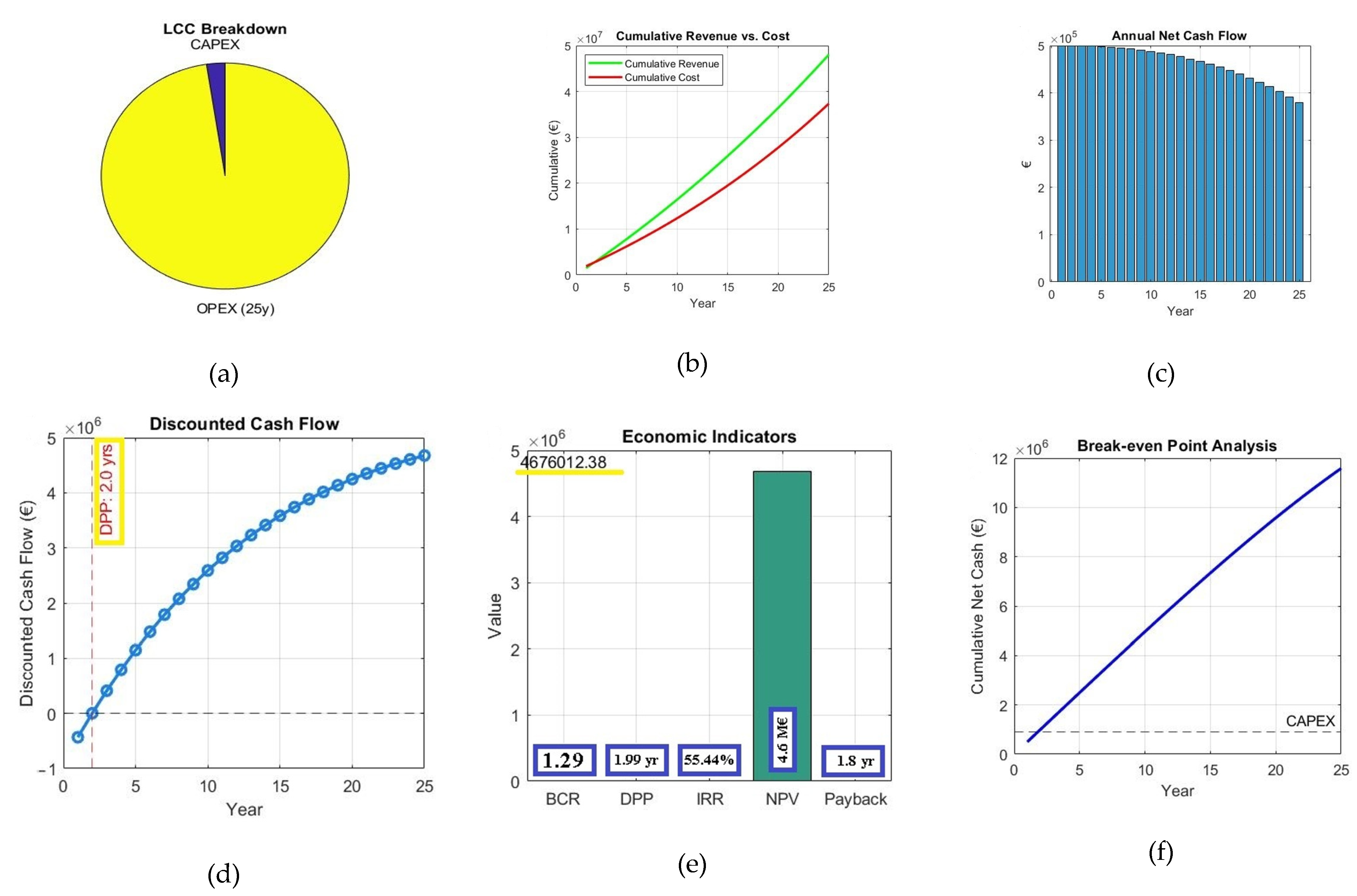
Figure 14 presents a comprehensive overview of the economic performance of the sludge-to-energy project under the given assumptions. In Figure 14a, the Life Cycle Cost (LCC) breakdown highlights that operational expenditures (OPEX) over the 25-year lifetime significantly dominate the overall cost structure, while capital expenditure (CAPEX) constitutes a minor portion. This reflects a typical scenario where the investment is relatively modest upfront, but long-term operational efficiency plays a critical role in economic viability.

Figure 14b illustrates the cumulative revenue and cost trends over the project lifetime. The cumulative revenue curve (green) consistently stays above the cumulative cost curve (red), indicating a growing financial surplus over time. This widening gap reflects the profitability of the project and aligns with the calculated net savings of EUR 10.69 million, confirming that revenues comfortably outweigh costs despite annual OPEX inflation.

Figure 14c depicts the annual net cash flow across the 25 years. Although there is a gradual decline due to OPEX increasing at 3% annually while revenue only grows at 2%, the net cash flow remains positive throughout the operational period. This persistent surplus ensures steady returns and supports the short payback timeframe.

Figure 14d shows the discounted cumulative cash flow, where the project surpasses the break-even point in present value terms after approximately 2 years. The indicated Discounted Payback Period (DPP) of 1.99 years confirms the speed at which the initial investment is recovered when the time value of money is considered. The curve continues to rise steeply, reflecting strong and sustained value generation. Figure 14e summarizes the key economic indicators. The project achieves a net present value (NPV) of EUR 4.68 million and an internal rate of return (IRR) of 55.44%, far exceeding the 7% discount rate, which signals excellent financial performance. A Benefit–Cost Ratio (BCR) of 1.29 indicates that for every euro invested, the project returns EUR 1.29 in benefits. The simple payback period is just 1.80 years, reinforcing the attractiveness of the investment. Lastly, Figure 14f illustrates the cumulative net cash flow over time and identifies the break-even point where cumulative earnings exceed the CAPEX. This occurs before year 2, in line with both the payback and DPP values. After break-even, the cumulative net cash rises linearly, confirming the system’s capacity to generate consistent profits well beyond the recovery of the initial investment.

Lastly, Figure 14a–f collectively demonstrates that the sludge-to-energy project, with free feedstock and favorable energy sales, is not only economically viable but also highly profitable. The combination of low CAPEX, rapidly recoverable investment, and high internal returns makes this model a promising and sustainable solution within the waste-to-energy domain.

4. Conclusions

Efficient sludge management is critical to the operation and cost-efficiency of wastewater treatment systems, as sludge handling constitutes a significant portion of operational expenses. This study highlights the energy potential of sludge as a component of sustainable solid waste management by leveraging the energy content of sludge from sewage treatment plants, particularly in industrial contexts, to support the development of a circular economy. By examining the waste-to-energy connection, this research investigates the properties of sludge relevant to energy generation, without proposing a comprehensive framework or detailed methodology for energy production from sludge, presenting it as a viable resource within refinery or treatment facility operations.

This study determined an average energy content of 3090 kcal/kg in sludge, showing a positive correlation with COD and a negative correlation with humidity. These findings highlight the energy potential of sludge, particularly from gas and oil refining processes, offering significant opportunities for reuse and energy recovery at the source.

Future research can focus on quantifying and analyzing the energy dynamics of industrial wastewater treatment facilities to further elucidate the role of sludge as an energy contributor. Extending this approach to investigate other valuable components, such as nitrogen and phosphorus, through systematic experimentation could also provide further insights into optimizing sludge utilization. This holistic approach to sludge management not only supports environmental sustainability but also promotes economic efficiency, presenting a dual benefit that aligns with the principles of a circular economy.