A Dynamic Model-Fitting Algorithm for Batch Laboratory Data: Application to Constant-Pressure Cake Filtration Experiments

Abstract

Model fitting of laboratory-generated experimental data is a foundational task in engineering, bridging theoretical models with real-world data to enhance predictive accuracy. This process is particularly valuable in batch dynamic experiments, where mechanistic models are often used to represent complex system behavior. Here, we propose a systematic algorithm tailored for the model fitting and parameter estimation of experimental data from batch laboratory experiments, rooted in a Process Systems Engineering framework. The paper provides an in-depth, step-by-step approach covering data collection, model selection, parameter estimation, and accuracy assessment, offering clear guidelines for experimentalists. To demonstrate the algorithm’s effectiveness, we apply it to a series of dynamic experiments on the pressure-constant cake filtration of calcium carbonate, where the pressure drop across the filter is varied as a key experimental factor. This example underscores the algorithm’s utility in enhancing the reliability and interpretability of model-based analyses in engineering.

1. Introduction

In engineering, experimental work is crucial because it relates theoretical knowledge and real-world applications. It helps engineers test and validate designs, gain deeper insights, and optimize existing technologies. Additionally, experimental work is essential for safety and risk mitigation, empirical data collection, and skill development [1]. Without  experimentation, engineering would lack the empirical foundation necessary to address the complex, dynamic, and often unpredictable challenges encountered in practice.

Experimentalists invest considerable effort into using experimental data for model fitting, as this process is fundamental for developing accurate representations of physical systems. These models are essential for prediction tasks such as process optimization and control. Model fitting transforms raw experimental data into mathematical models that describe underlying phenomena, requiring a combination of technical expertise, statistical knowledge, and  domain-specific experience. The goal is not only to capture the essence of the phenomena being studied but also to create reliable models for prediction, optimization, and control [2]. This careful and methodical approach ensures that the model serves as a dependable tool for advancing scientific understanding and supporting practical engineering applications.

In many engineering fields, experimental plans often involve batch experimentation, which provides time-varying data characterizing the process behavior over the course of the experiment. These dynamic data not only capture static features but also reveal crucial temporal patterns that are vital for forecasting trends and assessing risks. Fitting dynamic models to batch experiments is essential for understanding time-dependent systems. It helps optimize performance, enhances process control, and enables predictive capabilities. This step is vital for translating experimental data into actionable insights that inform the design and operation of dynamic processes [3]. By fitting models to dynamic data, experimentalists can convert complex, time-dependent information into predictive tools that guide decision-making, improve process safety, and drive innovation in fields such as chemical engineering, biotechnology, and environmental engineering.

The importance of data fitting for mechanistic models lies in its ability to refine, validate, and enhance first-principle models. By fitting experimental data to these models, their accuracy, reliability, and predictive power are significantly improved. This task is especially relevant in sequential experimental designs [4,5], where the interplay between experimental work and knowledge extraction through model fitting and parameter estimation is critical for optimizing system performance and minimizing experimental cost.

While numerous references address individual aspects of experimental design, model fitting, and parameter estimation, there remains a notable gap in the literature regarding the comprehensive integration of these activities. Specifically, there is a lack of guidance for experimentalists on how to navigate the entire process of transforming raw data into reliable models. This includes key decision-making steps and insights into the tools that can simplify the task.

This paper aims to bridge this gap by providing a unified, structured procedure for the complete workflow. We propose an algorithm designed to guide experimentalists through every stage, from data collection and model selection to model fitting, validation, and uncertainty analysis. By addressing this gap, we can streamline the process, enhance model accuracy, and ultimately facilitate the extraction of actionable insights from experimental data.

Novelty Statement and Organization

This paper introduces several novel contributions:

• A Process Systems Engineering-based algorithm for fitting experimental data from batch experiments to dynamic models;
• A comprehensive analysis of the key steps, decision points, and available tools necessary for effective model fitting;
• An application of the algorithm to a system in the field of Chemical Engineering—specifically, constant pressure cake filtration using calcium carbonate.

The paper is organized as follows. Section 2 provides background information and introduces the notation used to present the algorithm, which consists of four main stages: Data Preparation, Model Building and Consistency Analysis, Model Fitting, and Post-Analysis of Results. An  in-depth analysis of each stage is provided in Section 3. The  application of the algorithm to a real-world problem is detailed in Section 4, where experimental data from dynamic experiments of constant pressure cake filtration are used to fit a mechanistic model. Finally, Section 5 summarizes the findings and highlights the contributions of this work.

2. Notation and Background

In our notation, bold face lowercase letters represent vectors, bold face capital letters stand for continuous domains, blackboard bold capital letters are used to denote discrete domains, and capital letters are adopted for matrices. Finite sets containing $\iota$ elements are compactly represented by $〚\iota 〛\equiv \{1,\dots ,\iota \}$. The transpose operation of a matrix or vector is represented by “$\mathsf{T}$”, $\mathrm{hcat}(\mathbf{a},\mathbf{b})$ represents the horizontal concatenation of two vectors into one, $\mathrm{vcat}(\mathbf{a},\mathbf{b})$ stands for the vertical concatenation of vectors, $\mathrm{diag}\left(A\right)$ is the vector containing the diagonal elements of A, $\mathrm{card}$ is the cardinality of a domain, and $\mathrm{vec}\left(C\right)$ is the vectorization of the C, i.e., the operation that stacks all the columns of C into a single column.

In our conceptual framework, we adopt the terminology commonly used in Process Systems Engineering as in Hangos and Cameron [6] and Stephanopoulos [7]. We assume that the the experimental process, schematically represented in Figure 1, can be adequately described in mathematical terms by a state-space model. This formalism postulates that the complete behavior of the system can be represented by a finite set of differential and algebraic equations, connecting sets (classes) of variables, involving also a finite number of parameters (here considered to assume only constant numerical values, for easier distinction). The element on the left (a rectangle) of Figure 1 represents the experimental process itself, while the element on the right (a circle) depicts the measurement system that observes the process over the course of the experiment.

Let ${\mathbf{u}}^{\mathrm{var}}\in {\mathbb{R}}^{n_{i,v}}$ denote the vector of input variables (also called experimental factors) that vary over the experiment’s time horizon, $H\in {\mathbb{R}}_{\ge 0}$. Similarly, ${\mathbf{u}}^{\mathrm{fix}}\in {\mathbb{R}}^{n_{i,f}}$ is the vector of input variables that are fixed during an experiment but may vary across different experimental setups. Further, $\mathbf{x}\in {\mathbb{R}}^{n_s}$ represents the vector of state variables that dynamically characterize the system, and  $\mathbf{y}\in {\mathbb{R}}^{n_o}$ represents the vector of measured (or observed) variables over the experiment.

The parameter vectors are defined as follows: ${\mathit{\theta }}^{\mathrm{sta}}\in {\mathbb{R}}^{n_{\theta ,s}}$, which includes parameters in the state Equation (1a), and  ${\mathit{\theta }}^{\mathrm{mes}}\in {\mathbb{R}}^{n_{\theta ,m}}$, which includes parameters in the measurement Equation (2). Here, $\mathbf{f}:{\mathbb{R}}^{n_{i,v}+n_{i,f}+n_s+n_{\theta ,s}+1}\to {\mathbb{R}}^{n_s}$ is a vector of continuously differentiable functions defining the state equation and  $\mathbf{g}:{\mathbb{R}}^{n_{i,v}+n_{i,f}+n_s+n_{\theta ,m}}\to {\mathbb{R}}^{n_o}$ is a set of continuously differentiable functions defining the measurement equation.

Finally, the variable counts are defined as follows: $n_{i,v}$ is the number of time-varying input variables, $n_{i,f}$ is the number of fixed experimental factors, $n_s$ is the number of state variables, $n_o$ is the number of observed variables, $n_{\theta ,s}$ is the number of parameters in the state equation, and $n_{\theta ,m}$ is the number of parameters in the measurement equation.

The state equation for the model can be represented as

$$\begin{array}{cc}\hfill {\displaystyle \frac{\mathrm{d}\mathbf{x}}{\mathrm{d}t}}& =\mathbf{f}(\mathbf{x},{\mathbf{u}}^{\mathrm{var}},{\mathbf{u}}^{\mathrm{fix}},{\mathit{\theta }}^{\mathrm{sta}},t)\hfill \end{array}$$

(1a)

$$\begin{array}{cc}\hfill \mathbf{x}\left(0\right)& ={\mathbf{x}}^{\mathrm{ini}}\hfill \end{array}$$

(1b)

where (1a) describes the system dynamics and  (1b) specifies the initial conditions. Here, ${\mathbf{x}}^{\mathrm{ini}}\in {\mathbb{R}}^{n_s}$ represents the initial values of the state variables. Let $\mathit{\theta }\equiv \mathrm{hcat}({\mathit{\theta }}^{\mathrm{sta}},{\mathit{\theta }}^{\mathrm{mes}})\in {\mathbb{R}}^{n_{\theta ,s}+n_{\theta ,m}}$ denote the full parameter set for the state-space model. Generally, the parameters in ${\mathit{\theta }}^{\mathrm{mes}}$ are known a priori, so parameter estimation focuses on identifying ${\mathit{\theta }}^{\mathrm{sta}}$ within $\mathit{\theta }$.

The measurement equation is given by

$$\begin{array}{c}\hfill \mathbf{y}=\mathbf{g}(\mathbf{x},{\mathbf{u}}^{\mathrm{var}},{\mathbf{u}}^{\mathrm{fix}},{\mathit{\theta }}^{\mathrm{mes}},t),\end{array}$$

(2)

which relates the observed variables to the states, inputs, and known measurement parameters.

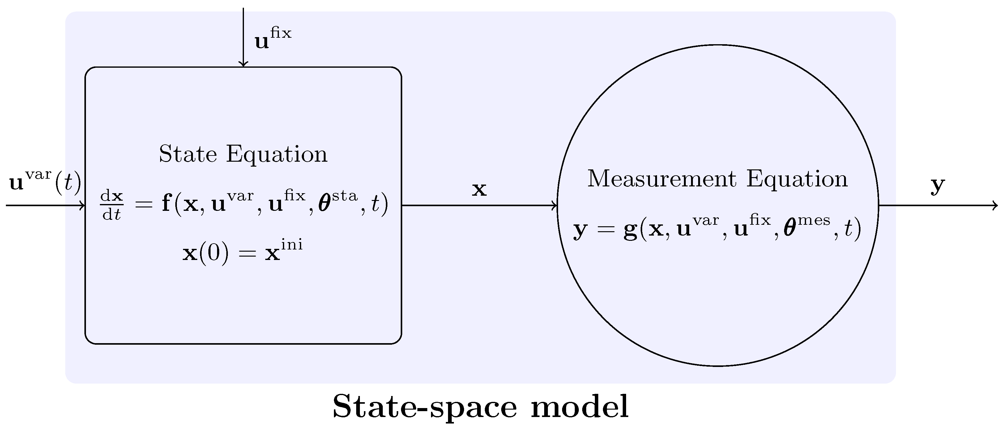
2.1. Conceptual Framework for Model Fitting from Experimental Data

In this section, we introduce the conceptual framework for model fitting, focusing on determining the parameter values that most accurately represent the observed system behavior. The model is mathematically represented by Equations (1) and (2), and it is assumed to accurately describe the system’s dynamics. Specifically, our goal is to identify the set of parameters ${\mathit{\theta }}^{\mathrm{sta}}\in \mathit{\theta }$ that optimally align with the experimental characteristics, assuming that the model structure is well-defined and consistent with mechanistic laws derived from conservation principles or a combination of these principles with empirical knowledge.

The fitting procedure is summarized in Figure 2 and comprises three sequential steps. While we focus on batch experiments, which are more common in laboratory settings, the procedure can be generalized to continuous processes.

The initial phase involves conducting experiments to observe the system’s dynamics, represented by $\mathbf{y}$, over a time horizon, H. Observations are taken at discrete time intervals, $t_i$, where each successive time $t_{i+1}$ is defined by $t_{i+1}=t_i+\Delta t_i$, with  $\Delta t_i>0$ as the sampling interval for the $i^{\mathrm{th}}$ observation. The data from the $j^{\mathrm{th}}$ experiment is structured as

$${\mathcal{E}}_j^{\mathrm{ori}.}={\{t_i,{\mathbf{u}}_i^{\mathrm{fix}},{\mathbf{u}}_i^{\mathrm{var}},{\mathbf{y}}_i\}}_{i\in 〚n_j〛},$$

where $n_j$ represents the number of observations in that experiment. In a multi-experiment framework, the results are consolidated into an extended dataset,

$${\mathcal{D}}^{\mathrm{ori}.}={\left[\mathrm{hcat}\left(\begin{array}{ccc}{\mathcal{E}}_1^{\mathrm{ori}.}& \cdots & {\mathcal{E}}_T^{\mathrm{ori}.}\end{array}\right)\right]}^{\mathsf{T}},$$

where T denotes the total number of experiments included for model fitting. This data collection process is part of the Data Collection module illustrated in Figure 2.

The second phase comprises the tasks of Data Preparation and Model Selection. The Data Preparation module focuses on preparing the dataset to ensure it is ready for model fitting; this process is discussed in detail in Section 3.1. Meanwhile, Model Selection and Structuring involves choosing a mathematical model, grounded in mechanistic principles, that accurately represents the system’s behavior. An additional necessary assumption of this formalism is that the underlying structure of the physical system can be uniquely identified from an appropriate set of measurements of both its input and output variables. Practical conditions to establish this property have been considered in the literature [3]. Although these tasks serve distinct purposes, they are addressed together in Section 3, as they are frequently performed concurrently.

The Data Preparation module applies several sequential operations to the dataset ${\mathcal{D}}^{\mathrm{ori}.}$, resulting in a refined dataset designated as ${\mathcal{D}}^{\mathrm{pre}.}\equiv {\left[\mathrm{hcat}\left(\begin{array}{ccc}{\mathcal{E}}_1^{\mathrm{prep}.}& \cdots & {\mathcal{E}}_T^{\mathrm{prep}.}\end{array}\right)\right]}^{\mathsf{T}}$, suitable for model fitting; the superscript “prep.” stands for prepared. It is important to note that the operations in Data Preparation may exclude records (or even entire experiments) from ${\mathcal{D}}^{\mathrm{ori}.}$; hence, we have $\mathrm{card}\left({\mathcal{D}}^{\mathrm{ori}.}\right)\ge \mathrm{card}\left({\mathcal{D}}^{\mathrm{pre}.}\right)$.

The task of Model Selection and Structuring involves defining a proposed model structure that accurately represents the system’s behavior, with  associated parameters informed by physics-based knowledge. Practically, this results in a state-space model—Equations (1) and (2)—denoted as $\mathcal{M}\left(\mathbf{y}\right|{\mathbf{u}}^{\mathrm{var}},{\mathbf{u}}^{\mathrm{fix}},\mathit{\theta },t)$. In choosing a model, several factors should be considered, including the following: (i) insights into process mechanisms, which help hypothesize relationships between variables; (ii) the model’s objectives—whether it is predictive, aimed at forecasting outcomes, or explanatory, focused on understanding relationships—as well as the balance between complexity and interpretability. The chosen model structure should align with established physical laws and theories relevant to the system, maintain dimensional consistency, and ensure that parameters are properly defined [8].

The third phase entails fitting the model to the data by estimating the optimal set of parameters, $\widehat{\mathit{\theta }}$, through an optimization method [9], which is conducted in the Model Fitting module. Typically, the accuracy of these parameter estimates is assessed by minimizing (or maximizing) the residuals, or differences, between observed data and model predictions (E) with respect to a given criterion. This step also provides statistical confidence intervals for the parameters, essential for reliable model-based predictions. Additionally, this process yields key outputs, including the prediction error and the Jacobian matrix at convergence, J, defined as [10]

$$J_{i,j}={\displaystyle \frac{\partial \mathcal{M}({\mathbf{y}}_i\mid {\mathbf{u}}_i^{\mathrm{var}},{\mathbf{u}}_i^{\mathrm{fix}},\mathit{\theta },t_i)}{\partial {\theta }_k}},i\in 〚n_j〛,j\in 〚T〛,k\in 〚n_{\theta }〛,$$

(3)

where this partial derivative represents the sensitivity of the model output at the ith data point in the jth experiment with respect to the kth parameter. The Jacobian matrix is subsequently employed for assessing parameter sensitivity, evaluating convergence stability during optimization, and constructing metrics for model fit quality. This phase is detailed in Section 3.2.

Finally, the fourth phase involves assessing the quality and adequacy of the fitted model to ensure predictive accuracy and evaluate how well its structure captures the essential characteristics of the process [11]. This phase, referred to as Results Post-Analysis, includes several subtasks, which are detailed in Section 3.3.

The primary goal is to verify that the model simulates the process with sufficient precision to enable sound decision-making in process control and optimization, focusing on quality diagnostics [12]. The  second goal is to examine how well the model structure reflects the underlying phenomenological aspects of the process, emphasizing model adequacy. Moreover, in a multi-experiment setting where fixed factors vary across experiments, we can investigate how model parameters depend on these factors. This analysis may reveal fundamental relationships, $\widehat{\mathit{\theta }}=\mathcal{G}\left({\mathbf{u}}^{\mathrm{fix}}\right)$, that enhance the physics-based insights conveyed by the model.

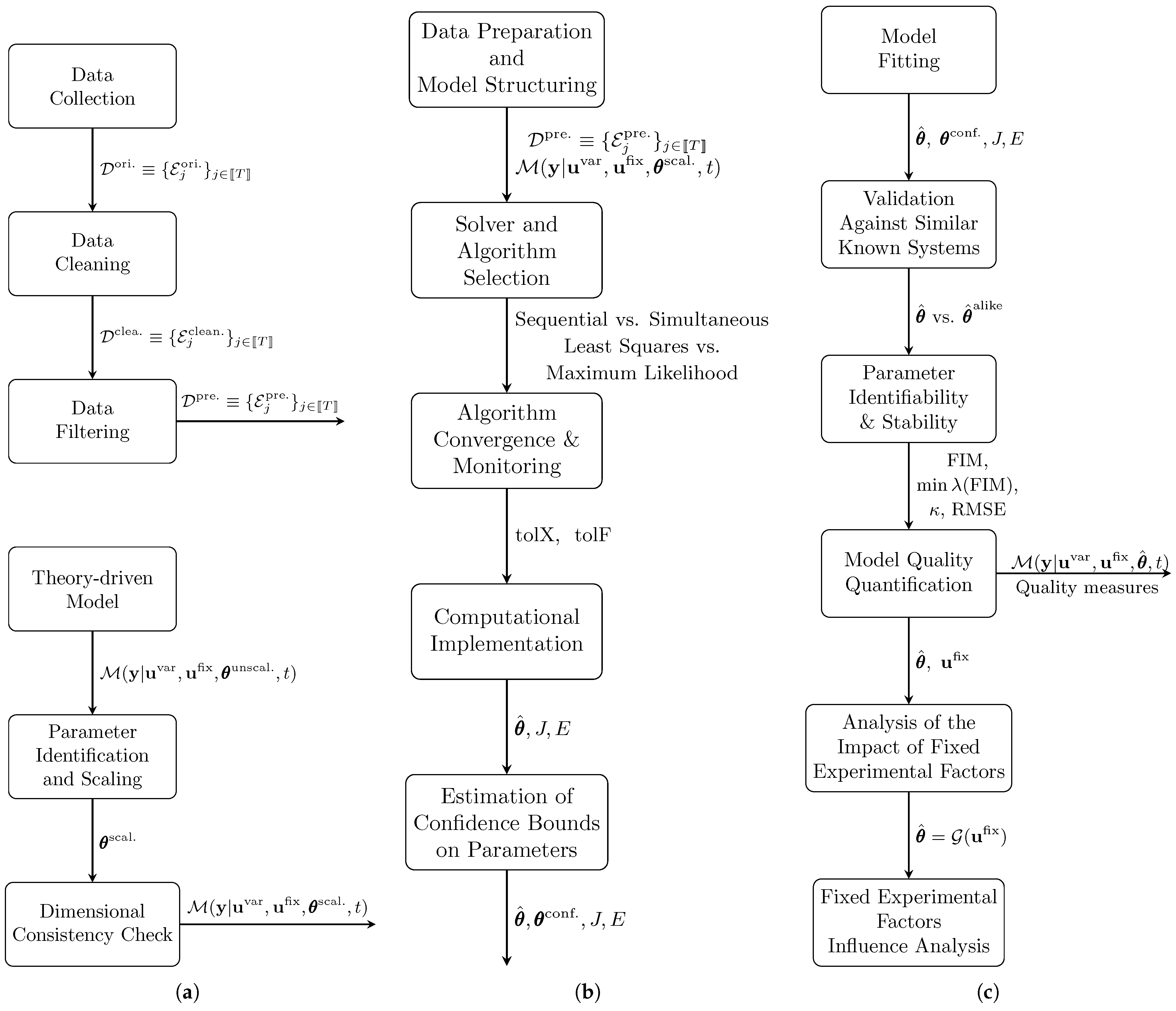
3. In-Depth Analysis of the Algorithm for Dynamic Model Fitting

In this section, we provide a detailed analysis of each component of the conceptual algorithm introduced in Section 2.1. Our approach to fitting mechanistic dynamic models to experimental batch laboratory data consists of three distinct phases: (i) data preparation and model selection; (ii) model fitting and confidence interval estimation for parameters; (iii) post-analysis of results, which includes assessing the impact of fixed factors on model parameters.

Here, our objectives are twofold: (i) to thoroughly examine each phase, highlighting the decisions the experimentalist must make to achieve accurate parameter estimates for the proposed model; (ii) to evaluate alternative approaches that may be more suitable in different contexts.

Figure 3 provide a detailed breakdown of each phase in the algorithm. Specifically, Figure 3a focuses on the Data Preparation and Model Selection modules, Figure 3b illustrates Model Fitting, and Figure 3c covers the Results Post-Analysis task.

3.1. Data Preparation and Model Selection

Figure 3a provides a schematic overview of the sequential tasks involved in Data Preparation and Model Selection. The process begins with Data Preparation, where experimental data are treated to ensure it is suitable for model fitting. Initially, the dataset, denoted as ${\mathcal{D}}^{\mathrm{ori}.}$, undergoes Data Cleaning, producing a cleaned dataset, ${\mathcal{D}}^{\mathrm{clean}.}$. This is followed by Data Filtering, which refines the cleaned data to reduce the impact of outliers, resulting in the final preprocessed dataset, ${\mathcal{D}}^{\mathrm{pre}.}$. Concurrently, Model Selection tasks are performed, including the selection and analysis of a model to describe the observed process behavior, the  identification and appropriate scaling of parameters and variables in the Parameter Identication and Scaling module, and an assessment of consistency with experimental data through the Dimensional Consistency Check module. The following sections detail each task, beginning with Data Preparation, then moving to the Model Selection and Structuring module.

3.1.1. Data Cleaning

Data cleaning addresses outliers, missing values, and errors that can disrupt the model-fitting process. Outliers may result from faulty observations or measurement inaccuracies, both of which can skew model predictions [13]. Additionally, missing values and errors introduce inaccuracies into the dataset [14]. A common approach to data cleaning is to remove outliers and handle missing values; however, this can lead to data loss and potential bias, especially in smaller datasets. Importantly, observations deviating from previous trends are not necessarily erroneous; they may indicate a different operational region. Such data points can offer valuable insights, potentially broadening the model’s applicability across a wider domain.

Among the techniques for removing outliers, we can identify the following: (i) the use of the Huber estimator and other robust statistical methods, including various M-estimators and S-estimators [15,16]; (ii) Robust regression methods [17]; (iii) Kalman filtering methods [18,19]; (iv) Wavelet transform methods [20,21]; (v) Bayesian approaches [22]; (vi) Deep-learning-based methods for sequential data [23,24].

In the context of time series analysis, missing values are defined as outlined by McKnight [25]. One common strategy for addressing these missing values is data imputation. However, in dynamic experiments, missing data can present significant challenges to maintaining the integrity of the time series. Imputation may often be perceived as interpolation of observations, which can distort the underlying patterns in the data, particularly when the missingness is not random. When employing imputation techniques, it is crucial to understand the nature of the missing data, specifically whether they are classified as Missing Completely At Random (MCAR), Missing At Random (MAR), or Missing Not At Random (MNAR) [26]. This classification will inform the choice of imputation method. Commonly used techniques include mean or median imputation [27], interpolation methods [28], and K-nearest neighbor imputation [29].

Typically, the Data Cleaning module does not involve scaling the data, as  preserving the original domain of the process response is important. However, if  needed, the model and its parameters can be scaled to improve consistency and minimize numerical issues during model fitting.

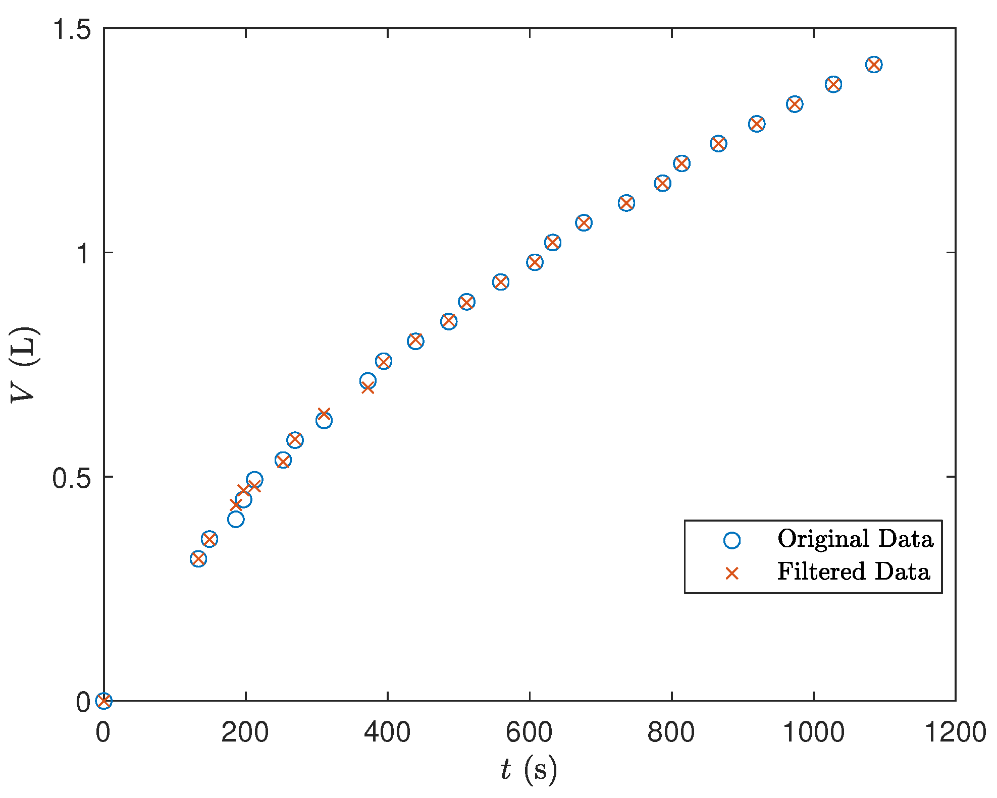
3.1.2. Data Filtering

Data filtering is a crucial process for enhancing the quality of raw data by systematically reducing noise, addressing outliers, and extracting meaningful patterns. This process ensures that the model accurately reflects genuine trends and relationships, rather than being skewed by irrelevant variations or measurement errors. Consequently, it prevents the model from fitting noise or anomalous values.

Several procedures can be implemented for data filtering: (i) Moving Average Filters: These filters smooth the data by averaging observations over a specified time (or other independent variable) window [30] (Chapters 14 and 15); this corresponds to a special case of local filtering (see below); (ii) Exponential Smoothing: Similar to the Moving Average Filters, these methods assign monotonically smaller weights to older observations in the averaging process [31]; (iii) Kalman Filter: A recursive filter designed to minimize the mean squared error between the predicted and observed states [32,33], based on an explicit system model; (iv) Nonparametric Filters: In contrast to the previous approach, this class of filters does not assume an underlying model structure for the system, or just makes minimal assumptions on the underlying statistical distribution of the system data [34]. This provides additional flexibility regarding the recognition of trends that might be present in the data but might not be well reproduced by fixed-structure models, such as the ones derived from a limited set of mechanistic principles; (v) Local filters such as Savitzky–Golay, median filters, LOESS/LOWESS: These filters use local models (sometimes corresponding to low order polynomials) to smooth the data, while having the capability to also preserve local features [35,36,37,38]; (vi) Frequency-Based Filters: These include band-pass filters [39] and Fourier filters [40], which target specific frequency components in the data; (vii) Wavelet Filters: These filters decompose data into multiple scales, facilitating filtering in both time and frequency domains [41]; (viii) Nonlinear Least Squares Filters: These filters employ nonlinear models to effectively filter out noise from the data [42].

These techniques can be effectively combined and applied to both the original signal and its derivatives, which can be obtained through numerical differentiation methods [43]. For examples of derivative filtering, refer to [44]. Recently, physics-informed knowledge filters have emerged as a powerful tool for enhancing data filtration [45,46]. These filters include fundamental physical principles to reduce noise by constraining dynamic trends. A notable application involves enforcing the sign of locally approximated derivatives of the signals based on established previous trends.

3.1.3. Theory-Driven Model

In this task, we develop mechanistic models that are both structurally consistent with conservation laws and capable of accurately describing the process behavior [47]. This involves the following [48]: (i) formulating a conceptual model that preserves the relationships among variables based on established theories; (ii) identifying key variables and defining their interrelationships. The output of this task is a model represented as $\mathcal{M}\left(\mathbf{y}\right|{\mathbf{u}}^{\mathrm{var}},{\mathbf{u}}^{\mathrm{fix}},{\mathit{\theta }}^{\mathrm{unscal}.},t)$ (see Figure 3a).

3.1.4. Parameter Identification and Scaling

Next, we identify the physical parameters to be fitted, as discussed by Himmelblau and Bischoff [49]. We analyze their physical interpretation and select appropriate scaling factors to normalize both parameter values and variables [50]. This normalization enhances numerical stability [51] and mitigates dimensional inconsistencies [52]. If prior knowledge or constraints on the parameters are available, we can incorporate them into the parameter estimation process using regularization techniques [53] or Bayesian approaches [54].

The result of this task is a consistent model, represented as $\mathcal{M}\left(\mathbf{y}\right|{\mathbf{u}}^{\mathrm{var}},{\mathbf{u}}^{\mathrm{fix}},{\mathit{\theta }}^{\mathrm{scal}.},t)$.

3.1.5. Dimensional Consistency Check

This task involves ensuring dimensional consistency across all terms in the model equations [3]. To achieve this, we need to (i) verify that units are clearly defined and that each equation maintains dimensional balance; (ii) assess the model’s plausibility and its adherence to fundamental principles, particularly conservation laws; and (iii) ensure that initial and/or boundary conditions are consistent and provided.

The outcome of this task is a consistent model that retains the same structure as described in Section 3.1.4.

3.2. Model Fitting

In this section, we describe the Model Fitting task schematically illustrated in Figure 3b. The inputs to this task are (i) the dataset ${\mathcal{D}}^{\mathrm{pre}.}$ and (ii) the model structure defined as a state-space model, $\mathcal{M}\left(\mathbf{y}\right|{\mathbf{u}}^{\mathrm{var}},{\mathbf{u}}^{\mathrm{fix}},{\mathit{\theta }}^{\mathrm{scal}.},t)$, as specified in the Model Selection and Structuring, and Data Preparation phase.

Model fitting is fundamentally an optimization problem [9,55], where the objective is to minimize a selected measure of residuals across all observations by adjusting parameter values—considered here as the decision variables of the optimization problem. This formalization requires an objective function, typically based on the chosen criterion for minimizing residuals, as well as the following constraints: (i) equality constraints that define the state-space model (Equations (1) and (2)) at each observation point; and (ii) inequality constraints to ensure the physical consistency of the state variables and to restrict parameter values within predefined ranges.

In multi-experiment scenarios with dynamic experiments, model fitting can be applied in two distinct ways (see Maiwald and Timmer [56] for a detailed discussion). The first approach assumes that all experiments share the same model structure and parameter set, allowing all experiments in ${\mathcal{D}}^{\mathrm{pre}.}$ to contribute to estimating a single set of parameters that best represents the entire dataset. This strategy involves solving a large optimization problem with relatively few parameters; however, convergence can be challenging, especially when experiments span different operating regimes.

The second approach treats each experiment independently, identifying an optimal set of parameters for each one. Here, each optimization run focuses exclusively on a single experiment, ${\mathcal{E}}_{j\in 〚T〛}^{\mathrm{pre}.}$, simplifying convergence for individual experiments. While this method requires repeating the optimization for all T experiments, it is advantageous when parameter values depend on experimental factors that remain constant within each experiment but vary across experiments.

The Model Fitting task includes several key steps, each essential for accurately estimating the model parameters:

• Solver and Algorithm Selection: Choose an appropriate algorithm and fitting criterion that align with the model structure and data.
• Algorithm Convergence and Monitoring: Define criteria to monitor convergence, ensuring that the optimization process reliably reaches a solution.
• Computational Implementation: Use a suitable computational tool to implement and solve the formulated optimization problem.
• Parameter Estimation and Confidence Interval Construction: Perform the optimization to estimate parameter values, along with constructing confidence intervals to assess parameter certainty.

Each of these steps is discussed in detail in the following sections.

Upon completion, the outputs of the numerical solution include the following: (i) optimal parameter estimates, based on the chosen fitting criterion; (ii) solution information from the solver, typically including the residuals between $\mathcal{M}\left(\mathbf{y}\right|{\mathbf{u}}^{\mathrm{var}},{\mathbf{u}}^{\mathrm{fix}},{\mathit{\theta }}^{\mathrm{scal}.},t)$ predictions and observations in ${\mathcal{D}}^{\mathrm{pre}.}$, along with a numerically approximated Jacobian using Equation (3); (iii) 95% confidence intervals for parameters derived from linear approximation theory [10,57].

3.2.1. Solver and Algorithm Selection

This task encompasses four distinct decisions, which will be addressed in the following paragraphs for clarity. These decisions include (i) selecting the optimality criterion; (ii) setting the signals to fit; (iii) choosing the numerical solution method; and (iv) choosing the optimization algorithm.

Choosing the Optimality Criterion

The optimality criteria commonly employed include the following: (i) Least Squares (LS)—This criterion minimizes the sum of squared differences between observed and predicted values, making it particularly effective for regression problems where the goal is to reduce large deviations. LS assumes homoscedasticity in the data (constant variance of errors) and is widely used in applications focused on minimizing outliers’ impact on the model fit [58,59]; (ii) Maximum Likelihood Estimation (MLE)—MLE maximizes the likelihood function, which reflects the probability of observing the data given the model parameters. It is especially flexible, allowing for the specification of data distribution assumptions, which makes it suitable for heteroscedastic data where variance changes with predictors. MLE not only fits the behavior of the process but also adjusts for variance in the data [60,61]; (iii) Average Relative Deviation (ARD)—This criterion minimizes the average of relative deviations between observed and predicted values. ARD is ideal for models where relative error is meaningful, such as in data with large ranges or when percentage accuracy is critical [62,63].

Consequently, this step involves selecting a single optimality criterion for the fitting process.

Selecting the Signals to Fit

Typically, two alternative approaches can be employed when deciding on the time dependency of the signals to fit. These approaches are summarized as follows:

• Integral Method: This approach directly utilizes the observed data (i.e., ${\mathcal{D}}^{\mathrm{pre}.}$) to fit the observations $\mathbf{y}$ over the time horizon of the experiments. In this method, the derivatives in the state Equation (1a) are approximated using a suitable numerical rule integrated within the solver, with the observational error arising from the measurement system. This method is analogous to the integral approach for parameterizing kinetic rate laws from kinetic data, as discussed by Levenspiel [64] and Himmelblau et al. [65]. In  this context, the signals to be fitted correspond to the accumulated values of the state variables, transformed through the measurement system at specified time points.
  Although this method can present numerical challenges, requiring an Ordinary Differential Equation (ODE) solver combined with an optimizer for the nonlinear least squares problem, it offers the significant advantage of fitting the data in a bias-free manner—without any prior treatment (see Schittkowski [66], Edsberg and Wedin [67] for relevant applications). Proper initialization of parameters is essential to ensure effective convergence of the optimizer, thus enhancing computational efficiency.
• Differential Method: Alternatively, the differential method fits the kinetic rates to increments in each reaction advance [68]. The model in this case is represented by algebraic rate equations, which can be linear or nonlinear, and generally facilitate a more straightforward least squares fitting process compared to the integral method. However, this approach necessitates numerical differentiation of the sampled data prior to fitting, a step that can be numerically challenging, especially with a large number of observed variables. This operation tends to amplify the error in the derivatives relative to the measurement error of the acquired signals [69]. Moreover, characterizing the error distribution becomes complex when the observations undergo local numerical differentiation. This method has been explored by Cremers and Hübler [70] and others.

Recently, Vertis [71] proposed a hybrid scheme that combines both methods for identifying reaction networks, which was later extended to batch sedimentation kinetics [72]. In this approach, experimental data undergo numerical differentiation and filtering before fitting with the differential method. The estimated parameters from this fitting serve as the initial solution for the integral method, which then fits the state space model to the data as it was collected.

Ultimately, a fitting strategy must be selected at the conclusion of this step.

Choosing the Numerical Solution Method

The primary algorithmic approaches for fitting dynamic models to experimental data include the following:

• Sequential Methods—These methods utilize an integrator to solve the state-space model, complemented by an outer optimization solver that iteratively refines the chosen optimality criterion. The integrator generates solutions based on a specified parameter set and computes parameter sensitivities, which are then used to approximate the objective function, gradient, and Hessian matrices for optimization. A Nonlinear Programming (NLP) solver—often based on techniques such as Generalized Reduced Gradient, Gradient Descent, or Sequential Quadratic Programming (SQP), iteratively adjusts the parameter vector until convergence is achieved. When the integrator’s solution grid does not match the observation times, interpolation is performed to align them. Although sequential methods are straightforward and tend to converge relatively quickly, they may struggle to maintain physically meaningful predictions for state and measurement variables, particularly when there is significant variability in state magnitudes [73].
  In essence, sequential methods alternate between an integrator (inner module) and an optimizer (outer module) until convergence is reached. Their main advantage lies in their simplicity; however, the convergence process can be sensitive, as predictions for states and measurements may become physically inconsistent due to the lack of constraints in the integrator. For a detailed review of sequential methods, see Vassiliadis et al. [74], Beck [75].
• Simultaneous Methods—These methods apply discretization techniques, such as orthogonal collocation on finite elements, to reformulate the differential model into algebraic equations corresponding to each experimental and observation time point. The transformed model is then solved as a single, large NLP problem [76,77,78], effectively converting it into a dynamic optimization problem focused on selecting the optimal parameter set for the desired criterion.
  Simultaneous methods offer improved control over state and measurement variables, ensuring that solutions remain within a physically meaningful range throughout the optimization process. However, their convergence rate is significantly influenced by the number of time points and experiments considered, as the complexity of the NLP tends to grow exponentially with additional observations, potentially leading to computational challenges due to NP-hard (Non-Polynomial time) characteristics. For an introduction to simultaneous methods, refer to Vasantharajan and Biegler [79], Tjoa and Biegler [80].

The parameterization of continuous state-space models is classified as a Dynamic Optimization (DO) problem. In this context, parameters are estimated by fitting the model to time-series data, with both state variables and parameters evolving according to the underlying system dynamics and constraints. Several techniques can be employed to tackle DO problems: (i) Simultaneous Methods: These methods alternate between integration and optimization steps. The control problem is approximated by parameterizing the control vector over the time horizon, which effectively reduces the infinite-dimensional problem to a finite-dimensional optimization problem over the control parameters [74]; (ii) Sequential Methods: This approach involves directly discretizing both state and control variables at collocation points across the entire time horizon. The differential equations are satisfied at these points, leading to a fully coupled system of algebraic constraints [81]; and (iii) Hybrid Methods: Hybrid methods transform a boundary value problem into an initial value problem, with one of the most common strategies being the multiple shooting method. The process begins by making initial guesses for the conditions, integrating the system forward in time. If the boundary conditions are not satisfied, adjustments are made to the initial guesses, and the integration is repeated until convergence is achieved [82].

All these methods can be effectively employed for model parameterization in dynamic models represented by continuous-time Differential Algebraic Equations (DAEs). For instance, the application of the multiple shooting method for parameter fitting is demonstrated in Kühl et al. [83].

At the conclusion of this task, a suitable numerical method should be selected.

Choosing the Optimization Algorithm

When addressing the optimization problem arising from model fitting, a variety of optimization algorithms and solvers can be employed. Examples of Nonlinear Programming (NLP) solvers include the following:

• Sequential Quadratic Programming (SQP), as implemented in MATLAB R2024b’s fmincon function [84].
• Trust Region and Conjugate Gradient Methods, which are utilized in Mathematica’s FindMinimum function [85].
• Interior Point (IP) Method, available through the IPOPT solver [86].
• Generalized Reduced Gradient (GRG) Method, used in the CONOPT solver [87].

For scenarios requiring global optimization, several tools can be considered, such as the Branch-and-Reduce Method implemented in BARON [88], or Multi-Start approaches, which are available in MSNLP [89]. Ultimately, the selection of an appropriate optimization algorithm is crucial for effectively solving the defined problem.

3.2.2. Algorithm Convergence and Monitoring

In this section, we establish the convergence criteria required for the algorithm to achieve convergence. Two primary criteria will be defined: (i) Function Tolerance (TolF): This criterion measures the maximum allowable change in the objective function value; (ii) Parameter Tolerances: These include absolute and relative tolerances, denoted as AbsTolX and RelTolX, respectively, which measure the maximum allowable change in the optimization parameters.

The parameter estimation problem frequently leads to multiple local optima, necessitating a post-analysis to evaluate these optima. This analysis should utilize physically informed knowledge to eliminate solutions that do not conform to conservation laws. In sequential methods, where an integrator is employed to solve the state-space model at local values of $\mathit{\theta }$, it is essential to impose tolerances on the integration algorithm, specifically relative and absolute tolerances. These algorithms should be capable of effectively handling stiff problems and Differential-Algebraic Equation (DAE) systems, often utilizing Backward Differentiation Formulas (BDFs). For a thorough discussion of these methods, readers are encouraged to refer to Hairer et al. [90]. To  maintain numerical consistency, the tolerances applied to the integrator must be smaller than those used for the optimization solver.

3.2.3. Computational Implementation

The computational implementation of tools for parameter fitting can be achieved using two primary approaches:

• General-Purpose Scientific Programming Languages: Languages such as Python, R, MATLAB, Julia, and  Mathematica are versatile and problem-oriented. They offer a wide range of up-to-date tools and libraries specifically designed for tasks such as numerical integration and optimization. These solutions are highly flexible and can easily integrate with other software, enabling more complex analyses that combine parameter fitting with various computational tasks. However, they do require programming skills to effectively utilize their capabilities.
• Specialized Parameter Fitting Tools: These tools are explicitly designed for parameter fitting and model optimization, often providing user-friendly applications suitable for non-programmers. They are tailored for specific types of application, enhancing usability. Examples of tools in this category include the following: (i) parmest: A module of Pyomo, a Python package that employs simultaneous methods through orthogonal collocation on finite elements for process optimization [91]; (ii) pyPESTO: A Python package focused on the parameter estimation of large, complex systems [92]; (iii) NonlinearFit: A built-in function in Mathematica for fitting nonlinear models [93]; (iv) dMOD: An R package designed for dynamic modeling and parameter estimation [94]; (v) Berkeley Madonna: An intuitive environment for graphically constructing and numerically solving mathematical equations [95].

At the conclusion of this stage, the implementation should yield the optimal set of parameters, $\widehat{\mathit{\theta }}$, along with additional information obtained after convergence, including the prediction error, E, and the Jacobian of the optimization problem, J, as defined by Equation (3).

3.2.4. Estimation of Confidence Bounds on Parameters

There are several methods for computing confidence bounds for parameters in estimation procedures. The most commonly employed approaches include the following: (i) Frequentist Methods: This category includes techniques such as the Wald interval, which relies on the normal approximation of the estimator [96]. Additionally, it encompasses various bootstrapping methods that use resampling techniques to estimate the sampling distribution of the estimator and construct confidence intervals, as demonstrated in Haraki et al. [97]; (ii) Asymptotic Methods: These methods include the normal approximation, which leverages the central limit theorem to approximate the distribution of the estimator as normal for large samples [10].

Asymptotic methods are often favored because they can be applied in a broader range of contexts beyond the Wald method, including variance estimation in more complex scenarios, and they offer confidence intervals within wider statistical frameworks. In contrast, bootstrapping methods may pose challenges due to their computational demands. These factors collectively favor the use of asymptotic methods, even though they may overlook the effects of nonlinearities on confidence bounds, as they depend on local linear approximations of the nonlinear model.

The asymptotic estimation of the 100 (1 − α) % confidence intervals for $\widehat{\mathit{\theta }}$ begins with the calculation of the normalized variance-covariance matrix, given by $C=n^{-1}{\left(J^{\mathsf{T}}J\right)}^{-1}$. Next, the standard errors of the parameters are computed using $\mathbf{SE}\left(\widehat{\mathit{\theta }}\right)=\sqrt{\mathrm{diag}\left(C\right)}$. Finally, the confidence intervals for the $n_{\theta }$ parameters are established using the relation

$$[\widehat{\mathit{\theta }}-z_{\alpha /2}\mathbf{SE}\left(\widehat{\mathit{\theta }}\right),\widehat{\mathit{\theta }}+z_{\alpha /2}\mathbf{SE}\left(\widehat{\mathit{\theta }}\right)],$$

(4)

where $z_{\alpha /2}$ is the critical value from the standard normal distribution that corresponds to half of the desired confidence level.

At the conclusion of this analysis, we determined the optimal parameter set along with their asymptotically normal confidence intervals.

3.3. Results Post-Analysis

In this section, we analyze the Results Post-Analysis, which is schematically represented in Figure 3c. The inputs for this phase include (i) the parameter estimates, $\widehat{\mathit{\theta }}$, along with their confidence intervals and (ii) the prediction error, E, and the Jacobian matrix, J. These inputs are obtained from the Model Fitting task.

The Results Post-Analysis phase encompasses several key subtasks that are crucial for assessing the quality and reliability of the fitted model. This step ensures that the model is not only mathematically sound but also meaningful for prediction and knowledge generation. The main subtasks are as follows:

• Physical Validation Against Similar Known Systems: This involves comparing the estimated parameters with those reported for similar systems in the literature.
• Parameter Identifiability and Stability Analysis: This step checks if the parameters can be estimated uniquely and measures its numerical stability and collinearity.
• Model Quality Quantification: This measures the model’s predictive accuracy.

When experimental fixed factors vary across the set of experiments, further analysis on the dependence of parameters on these factors is necessary to identify any relationships not captured by the model. Thus, two additional tasks are performed:

4.

Analysis of the Impact of Fixed Experimental Factors: This task involves regressing the parameters against the fixed factors used in the experiments.

5.

Fixed Experimental Factors Influence Analysis: This step analyzes the results from the regression to derive additional insights.

Each of these tasks is discussed in detail in the following sections.

3.3.1. Physical Validation Against Similar Known Systems

This task involves analyzing the results—specifically the parameter estimates and their corresponding confidence intervals—by referencing similar systems for which data are available. This process typically takes advantage of knowledge transfer among physically similar systems, providing an initial qualitative perspective on model accuracy [98]. By contrasting the parameter estimates with values reported for comparable systems, one can assess the plausibility and realism of the findings. Identifying discrepancies serves as a valuable step for model refinement, while confirming estimated values enhances credibility, demonstrating that the model is not only mathematically consistent but also applicable for predictive purposes.

3.3.2. Parameter Identifiability and Stability Analysis

Measuring practical (and global) identifiability directly is challenging, especially in complex or nonlinear models. Identifiability corresponds to the ability to uniquely estimate model parameters from the available data [99], ensuring that the estimated parameters accurately reflect the underlying processes and can be distinguished based on the observed data. Identifiability can be assessed through the following methods: (i) Sensitivity Analysis: Evaluates how sensitive the model is to small changes in parameter values; (ii) Eigenvalue Analysis of the Fisher Information Matrix (FIM): The smallest eigenvalues indicate directions in parameter space where information is low, highlighting potential identifiability issues; (iii) Profile Likelihood: This method involves fixing the parameter of interest at various values and re-estimating the other parameters to maximize the likelihood, thereby assessing the uncertainty around the parameter estimates.

In addition to these techniques, identifiability can be assessed using common metrics that also evaluate parameter stability [100]. These metrics include the following:

• Inter-Parameter Correlation: High correlations between parameters may indicate linear dependence or redundancy, which can lead to increased instability in parameter estimates [101].
• Condition Number of the Fisher Information Matrix (FIM): A high condition number suggests that the sensitivity matrix is close to singular, indicating that small changes in the data can significantly influence parameter estimates [59,102].
• Variance Inflation Factor (VIF): Elevated VIF values signal that parameters are not sufficiently determined by the data, leading to increased variance in parameter estimates due to multicollinearity [103].

Next, we present the equations utilized to compute these metrics for evaluating parameter stability. Let B be a diagonal square matrix of size $n_{\theta }$ containing the square roots of the diagonal elements of the covariance matrix C. The correlation matrix of the parameter estimates is then defined as $R=B^{-1}C{B}^{-1}$. The element $R_{i,j}$ indicates the cross-correlation between the ith and jth parameters, with all diagonal elements equal to $1.0$.

The Variance Inflation Factor (VIF), denoted mathematically as ${\upsilon }_{i,j}$, quantifies the degree of collinearity between pairs of parameters and is calculated using the formula ${\upsilon }_{i,j}={(1-R_{i,j}^2)}^{-1}$. The condition number $\kappa$ can be derived from either the covariance matrix, C, or its equivalent Fisher Information Matrix (FIM), F, given that $C\approx F^{-1}$. It is specifically computed as $\kappa ={\lambda }_{max}\left(C\right)/{\lambda }_{min}\left(C\right)$, where ${\lambda }_{max}\left(C\right)$ and ${\lambda }_{min}\left(C\right)$ represent the maximum and minimum eigenvalues of the covariance matrix, respectively. Additionally, other measures based on the FIM can also be employed to assess parameter stability and information content in the dataset, such as the minimum eigenvalue, which is commonly used in this context [104].

Guidelines for orthogonality analysis have been established by Belsley et al. [100] and López et al. [12], who propose practical cut-off values: an absolute maximum parametric correlation of $0.95$ and a condition number threshold of 20. Although these thresholds are somewhat arbitrary, they provide useful benchmarks for assessing model fitting performance, as discussed in Duarte et al. [105].

3.3.3. Model Quality Quantification

In this step, we evaluate the quality of the model in capturing the behavior of the process. The quality metrics focus on how well the model represents the data and their predictive capabilities. While various classes of metrics can be applied to empirical models, only a select few are recommended for mechanistic models. For instance, correlation is not commonly employed in this context because mechanistic models are designed to accurately reflect the dynamics of the system over time rather than to represent overall trends or associations between variables. Among the quality measures used for mechanistic models are the following:

• Goodness-of-Fit Metrics based on prediction errors;
• Parameter Sensitivity and Identifiability Analysis, as discussed in Section 3.3.2;
• Information Criteria, such as the Akaike Information Criterion, which balance model fidelity with parsimony and are commonly used for model discrimination.

Since our emphasis is on model fitting rather than model discrimination—and considering that we only have a plausible model structure to work with—we will focus on a single measure from the Goodness-of-Fit Metrics: the Root Mean Squared Error (RMSE). For a single experiment with $n_j$ time observations of $n_o$ observed variables, the RMSE is defined as

$$RMSE=\sqrt{{\displaystyle \frac{\mathrm{vec}{\left(E\right)}^{\mathsf{T}}\mathrm{vec}\left(E\right)}{n_j{n}_o}}}.$$

(5)

This equation highlights the importance of appropriately scaling the variables, and its adaptation for multiple experimental fitting setups is straightforward.

3.3.4. Analysis of the Impact of Fixed Experimental Factors

In experiments involving multiple runs where certain factors are held constant (denoted as ${\mathbf{u}}^{\mathrm{fix}}$), it is essential to investigate any potential relationships between these fixed factors and the model parameters, $\mathit{\theta }$ [106]. Such relationships are often empirical in nature, frequently modeled as power laws or similar representations. An  alternative approach to capture this dependence is through multi-level or hierarchical modeling techniques, which allow for the integration of both fixed and random effects across different experimental conditions.

3.3.5. Influence of Fixed Experimental Factors on Parameter Estimation

In this analysis, we explore the existence of relationships between parameters and fixed experimental factors by regressing $\widehat{\mathit{\theta }}=\mathcal{G}\left({\mathbf{u}}^{\mathrm{fix}}\right)$, where $\mathcal{G}:{\mathbb{R}}^{i,f}\mapsto \mathbb{R}$ represents an empirical function. To enhance the robustness of our analysis, we can compute confidence intervals for the estimated parameters (see Section 3.3.2) as well as assess the correlation coefficient, given that $\mathcal{G}$ is typically linear or can be linearized with respect to ${\mathbf{u}}^{\mathrm{fix}}$.

4. Application of the Algorithm for Dynamic Model Fitting

In this section, we illustrate the application of the algorithm for Dynamic Model Fitting introduced in Section 3. We conducted a series of 36 laboratory batch experiments to investigate the filtration characteristics of an incompressible cake using a constant pressure setup. All experiments utilized commercial analytical-grade calcium carbonate (CaCO₃) particles (full specification: Calcium carbonate agr, reag.ph.eur., Labbox Export, Barcelona, Spain). The calcium carbonate has a molecular weight of $100.09$ Da, a bulk density of $0.760$ g/cm³, and complies with identification standards A and B. The  average particle diameter was measured at 4.51 μm, while the particle density, determined by helium pycnometry with an AccuPyc 1330 Pycnometer (Micromeritics, Norcross, GA, USA), was found to be ${\varrho }_p=2.5327$ g/cm³.

The experiments were performed using distilled water at a temperature of approximately 25 °C. Under these conditions, the density and viscosity of the water were measured as ${\varrho }_l=0.997$ g/cm³ and ${\mu }_l$ = 8.891 × 10⁻⁴ Pa·s, respectively.

The concentration of CaCO₃ in the experimental suspension was set at 111 g/L and is treated as a fixed experimental factor, remaining constant across all experiments. In contrast, the pressure drop across the filter is maintained at a constant value during each individual experiment, but it varies between different experiments. Specifically, $n_{i,f}=1$, and  ${\mathbf{u}}^{\mathrm{fix}}$ is a vector containing a single element, $\mathrm{vec}(\Delta P)$, representing the pressure drop applied to the filter. The observational error of the measurement system is ±1.0 mL.

In cake filtration, critical parameters include filter cake resistance and filter medium resistance. Although filter cakes are often assumed to be incompressible, these two parameters are essential for characterizing the suitability of materials for filtration. Typically, all other variables are predetermined based on the experimental conditions [107]. The  assumption of incompressibility relies on the material properties of the cake and the operational conditions. Our goal is to parameterize both the filter cake and filter medium resistance using the experimental data obtained from this multi-experiment setup. To mathematically represent the filtration process, we employ a dynamic model grounded in conservation laws.

In constant-pressure cake filtration, a porous layer called the “cake” forms from suspended materials in the feed slurry. As filtration continues, solids from the liquid suspension accumulate on the filter medium, building up the cake layer. This layer acts as a barrier, effectively retaining particles while allowing the liquid to pass through, thereby separating solids from the liquid phase [108]. Despite being a well-established process, cake filtration remains an active area of research, especially in the design of industrial filtration units [109,110]. For  instance, Kuhn et al. [111] specifically examined methodologies for parameter estimation in incompressible cake filtration experiments.

Next, we briefly describe the actions taken in each phase of the algorithm for Dynamic Model Fitting.

4.1. Data Preparation and Model Selection

This section outlines the actions performed in the Data Preparation and Model Selection module. To introduce the terminology used in the Data Preparation module, we start with the Model Building and Consistency Checking task.

4.1.1. Model Building and Consistency Checking

To develop a mechanistic model for the process, we decompose the overall pressure drop across the filter, $\Delta P$, into two distinct components [111,112]:

• the pressure drop across the cake, $\Delta P_c$;
• the pressure drop across the filter medium, $\Delta P_f$;

Such that $\Delta P=\Delta P_c+\Delta P_f$.

We can then use Darcy’s law to express $\Delta P_c$ as

$$\Delta P_c={\displaystyle \frac{Q\mu H}{Ak}}={\displaystyle \frac{\mu Hr}{A}}Q={\displaystyle \frac{\mu rVK}{A^2}}{\displaystyle \frac{\mathrm{d}V}{\mathrm{d}t}},$$

(6)

where Q is the volumetric flow rate, also represented by ${\displaystyle \frac{\mathrm{d}V}{\mathrm{d}t}}$; $\mu$ is the dynamic viscosity; H is the cake height; A is the filter’s cross-sectional area; r is the height-specific (cake) resistance (one of the parameters to fit); K is the concentration constant; k is the permeability; and V is the volume of fluid filtered.

By applying Darcy’s law to the filter medium, we derive the expression for the pressure drop across it,

$$\Delta P_f={\displaystyle \frac{Q\mu R_f}{A}}={\displaystyle \frac{\mu R_f}{A}}{\displaystyle \frac{\mathrm{d}V}{\mathrm{d}t}},$$

(7)

where $R_f$ is the resistance of the filter medium, another parameter to be estimated. Through algebraic manipulation, we obtain the following ODE representing the process dynamics,

$$\begin{array}{cc}\hfill {\displaystyle \frac{\mathrm{d}V}{\mathrm{d}t}}& ={\displaystyle \frac{\Delta P{A}^2}{\mu (rKV+R_{f}A)}},\hfill \end{array}$$

(8a)

$$\begin{array}{cc}\hfill V\left(0\right)& =0,\hfill \end{array}$$

(8b)

where Equation (8a) is the state equation with $n_s=1$ and $\mathbf{x}\equiv \mathrm{vec}\left(V\right(t\left)\right)$, indicating that the state vector consists solely of the filtered volume. Equation (8b) specifies the initial condition.

The specific cake resistance, r, is an intrinsic property that characterizes the behavior of the cake throughout the consolidation process. It is commonly estimated using a modified form of the Almy–Lewis equation [113],

$$r=r_0\Delta P^{{\gamma }_c},$$

(9)

where $r_0$ is the reference resistance of the cake, ${\gamma }_c$ denotes the compressibility index, and $\Delta P$ is the applied pressure. For  incompressible cakes, ${\gamma }_c\to 0$ [114], indicating that estimating ${\gamma }_c$ can help verify whether or not the cake may indeed be considered incompressible. A similar formulation applies to the filter medium resistance:

$$R_f=R_{f,0}\Delta P^{{\gamma }_f}.$$

(10)

These empirical relationships suggest a dependence of the fitted parameters on the pressure drop. As a result, parameters estimated at different pressure drops are expected to vary, reinforcing the approach of fitting unique parameter sets for each experiment rather than relying on a single global set that represents an average behavior. Here, we designate $r_0$ and $R_{f,0}$ as the reference resistances for the cake and filter medium, respectively (i.e., their values at zero pressure drop), and ${\gamma }_c$ and ${\gamma }_f$ as their respective compressibility indices.

The observed variable in this process is the cumulative volume of filtrate collected, so $n_o=1$ and $\mathbf{y}\equiv \mathrm{vec}\left(V\right(t\left)\right)$, meaning that $y_1\left(t\right)=x_1\left(t\right)$, or equivalently:

$$V^{\mathrm{meas}.}\left(t\right)=V\left(t\right).$$

(11)

In the Parameter Identification and Scaling step we define the vector of parameters to be estimated—i.e., $\mathit{\theta }\equiv \mathrm{vec}(r,R_f)$, with $n_{\theta }=2$.

In the Dimensional Consistency Check phase, we standardized the units for the parameters and process variables. To align with the units of the acquired signals (see Section 4.1.2), time t is expressed in seconds (s), the fixed experimental factor $\Delta P$ in Pascal (N/m²), and the accumulated volume V in liters (L).

The constants used are $A=2.717 {\mathrm{dm}}^2$, $\mu =8.891\times {10}^{-4} \mathrm{Pa}·\mathrm{s}$, and  $K=0.111 {\mathrm{kg}}_{\mathrm{solids}}/\mathrm{L}$. Consequently, the  Dimensional Consistency Check phase indicated that the cake-specific resistance, r, should be expressed in dm · ${\mathrm{kg}}_{\mathrm{solids}}^{-1}$, and the filter medium resistance, $R_f$, in dm⁻¹. These units can, of course, be converted to standard SI units as needed.

To scale the parameters, we utilized existing knowledge of typical values for filter cake resistance and filter medium resistance specific to calcium carbonate, which are in the order of 1 × 10¹¹ m/kg and 1 × 10¹¹ m⁻¹, respectively [112] (Chapter 11). These values were adjusted for the units used in this study to facilitate parameter scaling. Consequently, we have:

$$\left(\begin{array}{c}r\\ R_f\end{array}\right)=\left(\begin{array}{c}1\times {10}^{12}{r}^{\mathrm{scal}.}\\ 1\times {10}^{10}{R}_f^{\mathrm{scal}.}\end{array}\right).$$

4.1.2. Data Preparation

The original datasets, each representing data collected from an individual experiment, j, contain the time points, $t_i$, at which the process was sampled, the accumulated filtered volume, $V_i$, and the pressure drop, $\Delta P_i$, applied during the experiment. Specifically, each experiment’s data can be represented as ${\mathcal{E}}_j^{\mathrm{ori}.}={\{t_i,\Delta P_i,V_i\}}_{i\in 〚n_j〛}$, where $j\in 〚T〛$, $T=36$, and the number of time points, $n_j$, varies across experiments. The complete dataset, ${\mathcal{D}}^{\mathrm{ori}.}$, is then formed by vertically concatenating the data from each experiment.

During the Data Cleaning phase, the dataset was refined by removing missing values and standardizing the measurement units. Additionally, data were organized to enhance interpretability, with experiments categorized into three pressure drop regimes:

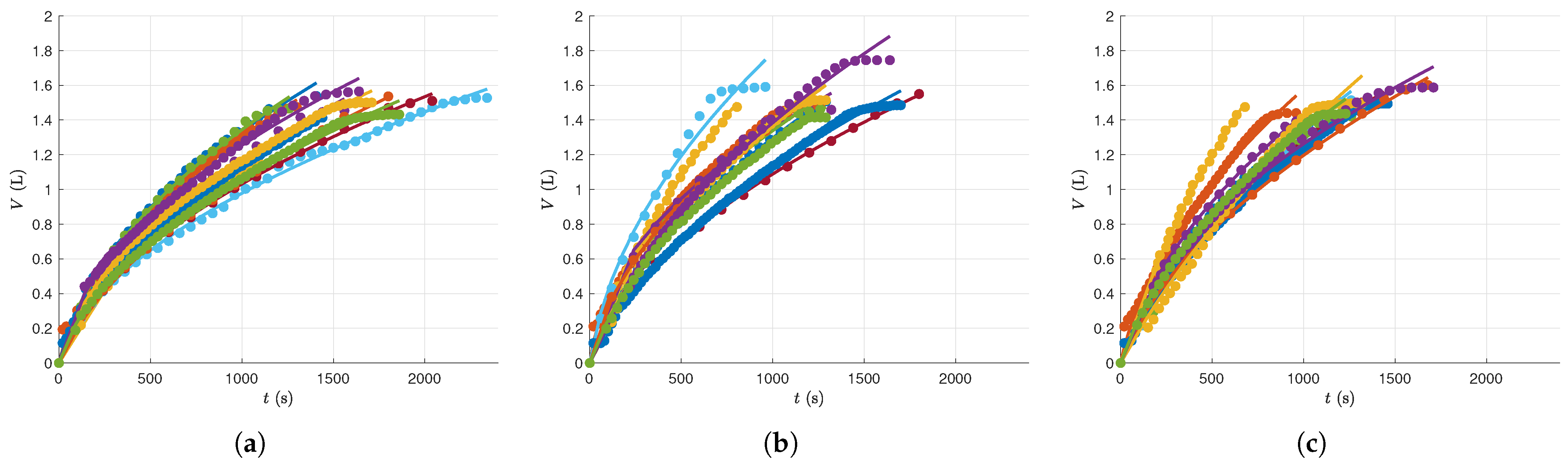
• Low-Pressure (LP) regime: spanning 32 × 10³ N/m² to 39 × 10³ N/m².
• Medium-Pressure (MP) regime: spanning 48 × 10³ N/m² to 52 × 10³ N/m².
• High-Pressure (HP) regime: spanning 63 × 10³ N/m² to 68 × 10³ N/m².

In total, 12 experiments were conducted within each pressure drop regime.

In the Data Filtration phase, a Savitzky–Golay filter with cubic polynomials and a window size of 7 time intervals was applied to each experiment’s data, smoothing the signal to reduce noise. Figure 4 illustrates the comparison between the original and filtered data for one experiment, showing the filter’s effect on data smoothing.

4.2. Model Fitting

This section details the decisions made during the Model Fitting phase. As outlined in Section 3.2, the first key task, Solver and Algorithm Selection, involved strategic choices for estimating parameters in the dynamic model (8a)–(11). We summarize these key decisions as follows:

• Optimality Criterion: Chose Least Squares.
• Signal to Fit: Used the measured variable, $V^{\mathrm{meas}.}\left(t\right)$, instead of its numerically differentiated form, employing the integral method.
• Numerical Solution Method: Adopted a simultaneous approach, with a variable-order, variable-step size integrator.
• Optimization Method: Selected the Interior Point-based NLP solver, IPOPT.

The choice of methods for demonstrating the algorithm was guided by the availability of well-established approaches in common packages, which can be easily used by non-expert users. Given the simplicity of the problem at hand, these methods were sufficient for our demonstration.

For the Algorithm Convergence and Monitoring task, we specified all necessary tolerances for the numerical solution, including those for model integration and the optimization algorithm:

• Integrator: AbsTolX = 1 × 10⁻⁷, RelTolX = 1 × 10⁻⁶.
• Optimization Solver: AbsTolX = 1 × 10⁻⁵, RelTolX = 1 × 10⁻⁵, TolF = 1 × 10⁻⁵.

For the Computational Implementation, the problem was coded in MATLAB, chosen for its robust numerical and graphical capabilities as well as its compatibility with IPOPT. The results are presented in Figure 5. Specifically, results for the Low-Pressure regime are shown in Figure 5a, for the Medium-Pressure regime in Figure 5b, and for the High-Pressure regime in Figure 5c. Solving the optimization problem to fit the model to each experimental dataset took less than 2 $\mathrm{s}$ of CPU time. All computations were performed on an Intel Core i7 machine with a $3.40$ $\mathrm{G}$$\mathrm{Hz}$ dual processor, running a 64-bit Windows 10 operating system. To emphasize the faster filtration rates at higher pressure drops, all plots are shown with the same axis scales.

At the end of the time window, we note that some of these experiments exhibit plateaus, where the total filtrate volume changes very slow. This corresponds to an experimental phase where the liquid in the solution has been nearly fully filtered, so that the operation can be interrupted at any moment. Continuing the operation in this region can induce higher compaction in the solid cake and therefore require a different system model, either with a different mathematical structure or keeping the same model structure but with distinct, and possibly time varying, numerical parameters. A systematic methodology to detect these structural changes, and simultaneously fit the corresponding individual models to each operating region, is described in [115]. This procedure can be applied when there is also interest in describing this terminal filtration phase. However, in the present study, its application to the system considered was not done due to the number of additional concepts that are required for its use, and because its presence in practice is not always significant, especially in industrial applications.

The parameter estimates and corresponding confidence intervals, as determined in the task Estimation of Confidence Bounds on Parameters, are shown in

Table 1. Parameters fitted for the set of experiments analyzed (fourth column contains the 95% confidence intervals for r, and the sixth column the 95% confidence intervals for $R_f$; Low stands for the lower bound and High for the upper bound).

Exper.	ΔP (N/m2)	r ($\times {\mathbf{10}}^{\mathbf{11}} \mathbf{m}/\mathbf{kg}$)	r CI [Low, High] ($\times {\mathbf{10}}^{\mathbf{11}} \mathbf{m}/\mathbf{kg}$)	${\mathit{R}}_{\mathit{f}}$ ($\times {\mathbf{10}}^{\mathbf{11}} {\mathbf{m}}^{-\mathbf{1}}$)	${\mathit{R}}_{\mathit{f}}$ CI [Low, High] ($\times {\mathbf{10}}^{\mathbf{11}} {\mathbf{m}}^{-\mathbf{1}}$)
1	3.2264 $\times {10}^4$	2.3146	[2.1606, 2.4686]	3.7834	[3.5016, 4.0652]
2	3.3331 $\times {10}^4$	2.1871	[2.0182, 2.3561]	1.6639	[1.2804, 2.0474]
3	3.4797 $\times {10}^4$	2.5676	[2.2621, 2.8732]	2.9014	[2.1930, 3.6098]
4	3.4997 $\times {10}^4$	2.1913	[2.0639, 2.3188]	2.3740	[2.1024, 2.6457]
5	3.5597 $\times {10}^4$	2.9005	[2.8345, 2.9665]	2.8232	[2.6849, 2.9616]
6	3.5597 $\times {10}^4$	3.3809	[3.2436, 3.5182]	2.9392	[2.6292, 3.2492]
7	3.5997 $\times {10}^4$	3.5768	[3.3794, 3.7741]	3.1109	[2.6494, 3.5725]
8	3.5997 $\times {10}^4$	2.8216	[2.6992, 2.9439]	1.5366	[1.2719, 1.8013]
9	3.7597 $\times {10}^4$	3.1750	[3.0389, 3.3111]	2.3418	[2.0218, 2.6618]
10	3.7730 $\times {10}^4$	2.2972	[2.1177, 2.4767]	2.2619	[1.8437, 2.6800]
11	3.7864 $\times {10}^4$	4.3398	[4.1490, 4.5306]	3.1502	[2.7023, 3.5981]
12	3.8663 $\times {10}^4$	2.9726	[2.7703, 3.1749]	4.5729	[4.0998, 5.0459]
13	4.8129 $\times {10}^4$	3.0327	[2.6027, 3.4627]	2.6811	[1.6217, 3.7405]
14	4.9063 $\times {10}^4$	3.2595	[3.1204, 3.3986]	5.7941	[5.4656, 6.1227]
15	4.9329 $\times {10}^4$	2.6321	[2.5357, 2.7285]	4.6420	[4.4331, 4.8509]
16	4.9329 $\times {10}^4$	2.8347	[2.7071, 2.9622]	4.6481	[4.3633, 4.9330]
17	4.9596 $\times {10}^4$	3.9359	[2.9593, 4.9125]	0.3571	[-2.0472, 2.7614]
18	5.1596 $\times {10}^4$	3.3371	[3.1695, 3.5047]	1.8606	[1.4992, 2.2220]
19	5.1596 $\times {10}^4$	1.8147	[1.3492, 2.2802]	2.1790	[0.9469, 3.4110]
20	5.1729 $\times {10}^4$	4.1960	[4.0354, 4.3566]	5.1684	[4.7914, 5.5453]
21	5.1996 $\times {10}^4$	1.2961	[1.1938, 1.3985]	4.5544	[4.3269, 4.7819]
22	5.1996 $\times {10}^4$	3.2009	[3.0649, 3.3369]	2.6465	[2.3314, 2.9616]
23	5.1996 $\times {10}^4$	2.3713	[2.1951, 2.5476]	5.0445	[4.6145, 5.4746]
24	5.1996 $\times {10}^4$	2.3215	[2.1398, 2.5033]	4.9016	[4.4270, 5.3761]
25	6.2662 $\times {10}^4$	3.1190	[2.9883, 3.2497]	5.4792	[5.2071, 5.7512]
26	6.4261 $\times {10}^4$	2.7145	[2.2419, 3.1872]	8.1022	[6.9989, 9.2055]
27	6.4661 $\times {10}^4$	3.0618	[2.7875, 3.3361]	4.8245	[4.1954, 5.4536]
28	6.4928 $\times {10}^4$	1.1126	[0.9813, 1.2439]	5.5838	[5.2820, 5.8856]
29	6.5061 $\times {10}^4$	2.5031	[2.2690, 2.7372]	7.9784	[7.4130, 8.5439]
30	6.5061 $\times {10}^4$	3.9471	[3.5709, 4.3233]	5.7260	[4.8261, 6.6259]
31	6.5328 $\times {10}^4$	4.0680	[3.7871, 4.3489]	6.7167	[6.0106, 7.4228]
32	6.5328 $\times {10}^4$	4.6175	[4.2955, 4.9395]	3.8817	[3.1316, 4.6317]
33	6.6661 $\times {10}^4$	1.7386	[1.2337, 2.2435]	10.3517	[9.0539, 11.6495]
34	6.7461 $\times {10}^4$	3.3915	[3.1592, 3.6238]	6.1191	[5.5825, 6.6557]
35	6.7994 $\times {10}^4$	2.7938	[2.5258, 3.0618]	4.1511	[3.5564, 4.7458]
36	6.8261 $\times {10}^4$	3.7190	[3.5805, 3.8574]	7.6443	[7.3176, 7.9711]

. For easier interpretation, they are arranged in order of increasing pressure drop. The results demonstrate consistency across experiments, with the exception of Experiment 17. In the following sections, “CI” denotes the confidence interval, where “CI [Low, High]” represents the lower bound as “Low” and the upper bound as “High”.

4.3. Results Post-Analysis

In this section, we analyze the quality of the estimation results. The task Physical Validation Against Similar Known Systems shows that the estimates align with the range of values reported in Couper et al. [112] (Chapter 11) for calcium carbonate cake filtration. The task Parameter Identifiability and Stability Analysis was performed by calculating the parameter identifiability and stability indicators outlined in Section 3.3.2. Similarly, the Model Quality Quantification task assessed the goodness-of-fit of the estimates, with results shown in

Table 2. Measures of parametric stability and goodness-of-fit.

Exper.	ΔP (N/m2)	${\mathit{R}}_{\mathit{r},{\mathit{R}}_{\mathit{f}}}$	VIF	$\mathit{\kappa }$	${\mathit{\lambda }}_{min}\left(\mathit{F}\right)$	RMSE
1	3.2264 $\times {10}^4$	−0.9748	20.0980	158.1123	2.9052 $\times {10}^{-3}$	7.5145 $\times {10}^{-3}$
2	3.3331 $\times {10}^4$	−0.9608	13.0063	135.7558	1.3677 $\times {10}^{-2}$	2.2602 $\times {10}^{-2}$
3	3.4797 $\times {10}^4$	−0.9550	11.3615	121.7498	5.1763 $\times {10}^{-3}$	2.3446 $\times {10}^{-2}$
4	3.4997 $\times {10}^4$	−0.9421	8.8939	84.0604	2.8280 $\times {10}^{-2}$	2.4280 $\times {10}^{-2}$
5	3.5597 $\times {10}^4$	−0.9534	10.9756	102.1270	2.2432 $\times {10}^{-2}$	1.1274 $\times {10}^{-2}$
6	3.5597 $\times {10}^4$	−0.9549	11.3527	117.1794	1.5192 $\times {10}^{-2}$	2.0411 $\times {10}^{-2}$
7	3.5997 $\times {10}^4$	−0.9534	10.9920	119.1352	4.0468 $\times {10}^{-3}$	1.4116 $\times {10}^{-2}$
8	3.5997 $\times {10}^4$	−0.9431	9.0382	87.2249	2.6145 $\times {10}^{-2}$	2.2809 $\times {10}^{-2}$
9	3.7597 $\times {10}^4$	−0.9576	12.0475	131.8749	1.6088 $\times {10}^{-2}$	2.1467 $\times {10}^{-2}$
10	3.7730 $\times {10}^4$	−0.9587	12.3682	133.7606	9.9214 $\times {10}^{-3}$	2.0488 $\times {10}^{-2}$
11	3.7864 $\times {10}^4$	−0.9515	10.5562	114.8954	6.9487 $\times {10}^{-3}$	1.9417 $\times {10}^{-2}$
12	3.8663 $\times {10}^4$	−0.9558	11.5722	125.5754	3.7082 $\times {10}^{-3}$	1.3586 $\times {10}^{-2}$
13	4.8129 $\times {10}^4$	−0.9804	25.8012	306.0901	2.4519 $\times {10}^{-3}$	2.4891 $\times {10}^{-2}$
14	4.9063 $\times {10}^4$	−0.9561	11.6393	128.1726	1.5580 $\times {10}^{-2}$	2.2008 $\times {10}^{-2}$
15	4.9329 $\times {10}^4$	−0.9506	10.3737	100.8583	7.8508 $\times {10}^{-3}$	9.4579 $\times {10}^{-3}$
16	4.9329 $\times {10}^4$	−0.9581	12.1878	124.1206	9.9176 $\times {10}^{-3}$	1.4923 $\times {10}^{-2}$
17	4.9596 $\times {10}^4$	−0.9721	18.1488	214.0123	1.7343 $\times {10}^{-3}$	4.3067 $\times {10}^{-2}$
18	5.1596 $\times {10}^4$	−0.9426	8.9729	86.1589	1.8085 $\times {10}^{-2}$	2.5913 $\times {10}^{-2}$
19	5.1596 $\times {10}^4$	−0.9542	11.1779	144.9213	1.3804 $\times {10}^{-2}$	6.7857 $\times {10}^{-2}$
20	5.1729 $\times {10}^4$	−0.9549	11.3413	123.7014	2.1587 $\times {10}^{-3}$	8.2544 $\times {10}^{-3}$
21	5.1996 $\times {10}^4$	−0.9608	13.0080	131.8937	1.5180 $\times {10}^{-2}$	1.4230 $\times {10}^{-2}$
22	5.1996 $\times {10}^4$	−0.9559	11.5822	124.0217	2.8913 $\times {10}^{-3}$	7.3362 $\times {10}^{-3}$
23	5.1996 $\times {10}^4$	−0.9603	12.8639	148.7153	1.2136 $\times {10}^{-2}$	2.4571 $\times {10}^{-2}$
24	5.1996 $\times {10}^4$	−0.9504	10.3407	131.1758	1.7813 $\times {10}^{-2}$	3.2612 $\times {10}^{-2}$
25	6.2662 $\times {10}^4$	−0.9520	10.6752	98.2779	5.0796 $\times {10}^{-3}$	9.9417 $\times {10}^{-3}$
26	6.4261 $\times {10}^4$	−0.9636	13.9890	152.1546	3.0048 $\times {10}^{-3}$	2.9569 $\times {10}^{-2}$
27	6.4661 $\times {10}^4$	−0.9729	18.6909	199.4043	2.1190 $\times {10}^{-3}$	1.3565 $\times {10}^{-2}$
28	6.4928 $\times {10}^4$	−0.9705	17.2193	183.9973	1.0443 $\times {10}^{-2}$	1.5392 $\times {10}^{-2}$
29	6.5061 $\times {10}^4$	−0.9593	12.5323	142.7233	3.9540 $\times {10}^{-3}$	1.7501 $\times {10}^{-2}$
30	6.5061 $\times {10}^4$	−0.9559	11.6063	130.1283	1.7841 $\times {10}^{-3}$	1.7123 $\times {10}^{-2}$
31	6.5328 $\times {10}^4$	−0.9559	11.6032	139.6985	1.8858 $\times {10}^{-3}$	1.4147 $\times {10}^{-2}$
32	6.5328 $\times {10}^4$	−0.9477	9.8105	105.3472	6.9158 $\times {10}^{-3}$	3.2597 $\times {10}^{-2}$
33	6.6661 $\times {10}^4$	−0.9638	14.0618	175.6443	8.3072 $\times {10}^{-3}$	6.0948 $\times {10}^{-2}$
34	6.7461 $\times {10}^4$	−0.9585	12.3097	131.4997	6.3333 $\times {10}^{-3}$	2.2281 $\times {10}^{-2}$
35	6.7994 $\times {10}^4$	−0.9541	11.1506	112.2819	1.2160 $\times {10}^{-2}$	3.4642 $\times {10}^{-2}$
36	6.8261 $\times {10}^4$	−0.9569	11.8662	130.5581	9.0935 $\times {10}^{-3}$	1.6653 $\times {10}^{-2}$

.

In Table 2, the third column presents the inter-parameter correlation between r and $R_f$, the fourth column shows the Variance Inflation Factor (VIF), the fifth provides the condition number of the Fisher Information Matrix (FIM), and the sixth contains the minimum eigenvalue of the FIM—all of which measure parameter stability and relate to model identifiability. The seventh column contains the RMSE, which serves as the measure of goodness-of-fit in this analysis.

The inter-parameter covariance, VIF, and condition number $\kappa$ indicate a substantial dependence between the parameters. Notably, r is inversely proportional to $R_f$; that is, as the filter cake resistance, r, increases, the filter medium resistance, $R_f$, decreases. The RMSE value demonstrates the model’s strong ability to capture the process behavior accurately.

In the task Analysis of the Impact of Fixed Experimental Factors, it is valuable to examine the effect of pressure drop on the parameters r and $R_f$. The primary goal is to evaluate the validity of the empirical Equations (6) and (7), enhancing our understanding of the cake’s characteristics. The approach involves taking the logarithm of the empirical relationships and performing a regression on the resulting linear forms:

$$\begin{array}{cc}\hfill ln\left(r\right)& =ln\left(r_0\right)+{\gamma }_{c}ln(\Delta P)\hfill \end{array}$$

(12a)

$$\begin{array}{cc}\hfill ln\left(R_f\right)& =ln\left(R_{f,0}\right)+{\gamma }_{f}ln(\Delta P)\hfill \end{array}$$

(12b)

Figure 6 presents the regression analysis of the parameters. A linear relationship between $ln\left(R_f\right)$ and $ln(\Delta P)$ appears plausible, while no such relationship is evident between $ln\left(r\right)$ and $ln(\Delta P)$. The results of our regression are summarized in

Table 3. Parameters fitted for Equation (12) and respective 95% confidence intervals.

Model	Reference Resistance	Reference Resistance CI [Low, High]	Compressibility Index	Compressibility Index CI [Low, High]	R2
Equation (12a)	25.9396	[25.8332, 26.0459]	0.0391	[−0.0672, 0.1455]	0.0010
Equation (12b)	12.2975	[12.1217, 12.4733]	1.3272	[1.1514, 1.5030]	0.2970

, which indicate the following: (i) There is no significant relationship between $ln\left(r\right)$ and $ln(\Delta P)$, as suggested by the correlation coefficient, which is close to 0, along with a low cake compressibility index; (ii) The hypothesized relationship between $ln\left(R_f\right)$ and $ln(\Delta P)$ is not strongly supported, with an $R^2$ value of 0.2970, despite a high medium compressibility index value (1.3272).

Finally, outlier detection using Huber’s method (see Section 3.1.1) identified two outlier experiments in the regression of $ln\left(r\right)$ vs. $ln(\Delta P)$ and one outlier in the analysis involving filter medium resistance. One of these outliers corresponds to Experiment 17, which was previously identified in Table 1.

5. Conclusions

In this work, we presented a structured and systematic approach for model fitting based on laboratory data, with a focus on batch dynamic experiments and mechanistic models that capture process dynamics. Our proposed methodology provides a comprehensive framework for experimentalists, guiding them through all stages of the model-fitting workflow—from data collection to post-analysis—while emphasizing optimal experimental design within budgetary constraints.

By addressing model accuracy, identifiability, and parameter stability, our approach bridges the tasks of model-fitting parameter estimation and model validation, which are crucial for deriving meaningful insights from experimental data. We analyzed each step of the workflow in depth, presenting methodological options, computational tools, and validation metrics to ensure model consistency and robustness.

To demonstrate the applicability of this approach, we applied it to a case study from Chemical Engineering: constant-pressure cake filtration with calcium carbonate, involving 36 experiments across three pressure regimes. While this application highlights its effectiveness in a traditional Chemical Engineering problem, the methodology is flexible and can be extended to other fields and various levels of model complexity.

The proposed algorithm is modular in design, allowing for the adjustment of tools, methods, solvers, and computational environments without significantly altering the overall workflow. While the current study serves as a conceptual demonstration, we do not anticipate difficulties in scaling the algorithm to larger datasets, including those from continuous processes or processes involving both mass and heat transfer phenomena. In such cases, we expect the primary impacts to be on CPU time and convergence, with no effect on the core functionality of the algorithm.

Overall, this structured approach provides experimentalists with a valuable tool for enhancing model reliability and gaining deeper insights into process behavior, paving the way for more efficient and informative experimental design in diverse engineering and scientific domains.

References

1. Doebelin, E. Engineering Experimentation: Planning, Execution, Reporting; McGraw-Hill Series in Mechanical Engineering; McGraw-Hill: New York, NY, USA, 1995. [Google Scholar]
2. Bevington, P.R.; Robinson, D.K. Data Reduction and Error Analysis for the Physical Sciences; McGraw-Hill: New York, NY, USA, 2003. [Google Scholar]
3. Ljung, L. System Identification: Theory for the User; Prentice Hall: Upper Saddle River, NJ, USA, 1999. [Google Scholar]
4. Marquardt, W. Model-based experimental analysis of kinetic phenomena in multi-phase reactive systems. Chem. Eng. Res. Des. 2005, 83, 561–573. [Google Scholar] [CrossRef]
5. Duarte, B.P.M.; Atkinson, A.C.; Granjo, J.F.O.; Oliveira, N.M.C. A model-based framework assisting the design of vapor-liquid equilibrium experimental plans. Comput. Chem. Eng. 2021, 145, 107168. [Google Scholar] [CrossRef]
6. Hangos, K.; Cameron, I. Process Modelling and Model Analysis; Process Systems Engineering; Academic Press: Cambridge, MA, USA, 2001. [Google Scholar]
7. Stephanopoulos, G. Chemical Process Control: An Introduction to Theory and Practice; Prentice-Hall International Series in the Physical and Chemical Engineering Sciences; Prentice-Hall: Upper Saddle River, NJ, USA, 1984. [Google Scholar]
8. Åström, K.J. Modelling and identification of power system components. In Realtime Control of Electric Power Systems: Proceedings of the Symposium on Real-Time Control of Electric Power Systems, Baden, Switzerland; Handschin, E., Ed.; Elsevier: Amsterdam, The Netherlands, 1972; pp. 1–28. [Google Scholar]
9. Bard, Y. Nonlinear Parameter Estimation; Academic Press: New York, NY, USA, 1974. [Google Scholar]
10. Seber, G.A.F.; Wild, C.J. Nonlinear Regression; John Wiley & Sons: New York, NY, USA, 2003. [Google Scholar]
11. Stewart, G.W. Collinearity and least squares regression. Stat. Sci. 1987, 2, 68–84. [Google Scholar] [CrossRef]
12. López, D.C.; Barz, T.; Korkel, S.; Wozny, G. Nonlinear ill-posed problem analysis in model-based parameter estimation and experimental design. Comput. Chem. Eng. 2015, 77, 24–42. [Google Scholar] [CrossRef]
13. Danuser, G.; Stricker, M. Parametric model fitting: From inlier characterization to outlier detection. IEEE Trans. Pattern Anal. Mach. Intell. 1998, 20, 263–280. [Google Scholar] [CrossRef]
14. Enders, C.K. Applied Missing Data Analysis; Guilford Publications: New York, NY, USA, 2022. [Google Scholar]
15. Huber, P.J. Robust estimation of a location parameter. Ann. Math. Stat. 1964, 35, 73–101. [Google Scholar] [CrossRef]
16. Miké, V. Efficiency-robust systematic linear estimators of location. J. Am. Stat. Assoc. 1971, 66, 594–601. [Google Scholar] [CrossRef]
17. Rousseeuw, P.J. Least median of squares regression. J. Am. Stat. Assoc. 1984, 79, 871–880. [Google Scholar] [CrossRef]
18. Schick, I.C.; Mitter, S.K. Robust recursive estimation in the presence of heavy-tailed observation noise. Ann. Stat. 1994, 22, 1045–1080. [Google Scholar] [CrossRef]
19. Tsai, C.; Kurz, L. An adaptive robustizing approach to Kalman filtering. Automatica 1983, 19, 279–288. [Google Scholar] [CrossRef]
20. Donoho, D.L.; Johnstone, I.M. Adapting to unknown smoothness via wavelet shrinkage. J. Am. Stat. Assoc. 1995, 90, 1200–1224. [Google Scholar] [CrossRef]
21. Mallat, S.G. Multiresolution approximations and wavelet orthonormal bases of L2(R). Trans. Am. Math. Soc. 1989, 315, 69–87. [Google Scholar] [CrossRef]
22. West, M.; Harrison, J. Bayesian Forecasting and Dynamic Models; Springer Science & Business Media: Berlin/Heidelberg, Germany, 2006. [Google Scholar]
23. Chalapathy, R.; Chawla, S. Deep learning for anomaly detection: A survey. arXiv 2019, arXiv:1901.03407. [Google Scholar] [CrossRef]
24. Brown, A.; Tuor, A.; Hutchinson, B.; Nichols, N. Recurrent neural network attention mechanisms for interpretable system log anomaly detection. In Proceedings of the First Workshop on Machine Learning for Computing Systems, Tempe, AZ, USA, 12 June 2018; Association for Computing Machinery: New York, NY, USA, 2018. [Google Scholar] [CrossRef]
25. McKnight, E. Missing Data: A Gentle Introduction; The Guilford Press: New York, NY, USA, 2007. [Google Scholar]
26. Curran, D.; Bacchi, M.; Schmitz, S.; Molenberghs, G.; Sylvester, R. Identifying the types of missingness in quality of life data from clinical trials. Stat. Med. 1998, 17, 739–756. [Google Scholar] [CrossRef]
27. Cleophas, T.J.; Zwinderman, A.H.; Cleophas, T.J.; Zwinderman, A.H. Missing data imputation. In Clinical Data Analysis on a Pocket Calculator: Understanding the Scientific Methods of Statistical Reasoning and Hypothesis Testing; Springer: Cham, Switzerland, 2016; pp. 93–97. [Google Scholar] [CrossRef]
28. Junninen, H.; Niska, H.; Tuppurainen, K.; Ruuskanen, J.; Kolehmainen, M. Methods for imputation of missing values in air quality data sets. Atmos. Environ. 2004, 38, 2895–2907. [Google Scholar] [CrossRef]
29. Zhang, S. Nearest neighbor selection for iteratively kNN imputation. J. Syst. Softw. 2012, 85, 2541–2552. [Google Scholar] [CrossRef]
30. Smith, S.W. The Scientist and Engineer’s Guide to Digital Signal Processing; California Technical Publishing: San Diego, CA, USA, 1997. [Google Scholar]
31. Holt, C.C. Forecasting seasonals and trends by exponentially weighted moving averages. Int. J. Forecast. 2004, 20, 5–10. [Google Scholar] [CrossRef]
32. Maybeck, P.S. Stochastic Models, Estimation, and Control; Academic Press: Cambridge, MT, USA, 1982. [Google Scholar]
33. Simon, D. Optimal State Estimation: Kalman, H-Infinity, and Nonlinear Approaches; Wiley-Interscience: Hoboken, NJ, USA, 2006. [Google Scholar]
34. Bowman, A.; Azzalini, A. Applied Smoothing Techniques for Data Analysis; Clarendon Press: Oxford, UK, 1997. [Google Scholar]
35. Savitzky, A.; Golay, M.J.E. Smoothing and differentiation of data by simplified least squares procedures. Anal. Chem. 1964, 36, 1627–1639. [Google Scholar] [CrossRef]
36. Huang, T.S.; Yang, G.J.; Tang, G.Y. A fast two-dimensional median filtering algorithm. IEEE Trans. Acoust. Speech Signal Process. 1979, 27, 13–18. [Google Scholar] [CrossRef]
37. Orfanidis, S.J. Introduction to Signal Processing; Prentice Hall: New Brunswick, NJ, USA, 1996; p. 798. [Google Scholar]
38. Simonoff, J.S. Smoothing Methods in Statistics; Springer: New York, NY, USA, 1996. [Google Scholar]
39. Haykin, S.; Van Veen, B. Signals and Systems, 2nd ed.; Wiley: New York, NY, USA, 2007. [Google Scholar]
40. Harris, F.J. On the use of windows for harmonic analysis with the discrete Fourier transform. Proc. IEEE 1978, 66, 51–83. [Google Scholar] [CrossRef]
41. Strang, G.; Nguyen, T. Wavelets and Filter Banks; Wellesley-Cambridge Press: Wellesley, MA, USA, 1996; p. 520. [Google Scholar]
42. Julier, S.J.; Uhlmann, J.K. Unscented filtering and nonlinear estimation. Proc. IEEE 2004, 92, 401–422. [Google Scholar] [CrossRef]
43. Ahnert, K.; Abel, M. Numerical differentiation of experimental data: Local versus global methods. Comput. Phys. Commun. 2007, 177, 764–774. [Google Scholar] [CrossRef]
44. Van Breugel, F.; Kutz, J.N.; Brunton, B.W. Numerical differentiation of noisy data: A unifying multi-objective optimization framework. IEEE Access 2020, 8, 196865–196877. [Google Scholar] [CrossRef] [PubMed]
45. Letzgus, S.; Müller, K.R. An explainable AI framework for robust and transparent data-driven wind turbine power curve models. Energy AI 2024, 15, 100328. [Google Scholar] [CrossRef]
46. Alabduljabbar, R.; Alshareef, M.; Alshareef, N. Time-aware recommender systems: A comprehensive survey and quantitative assessment of literature. IEEE Access 2023, 11, 45586–45604. [Google Scholar] [CrossRef]
47. Benvenuti, L.; De Santis, A.; Farina, L. On model consistency in compartmental systems identification. Automatica 2002, 38, 1969–1976. [Google Scholar] [CrossRef]
48. Biegler, L. Nonlinear Programming: Concepts, Algorithms, and Applications to Chemical Processes; MOS-SIAM Series on Optimization; Society for Industrial and Applied Mathematics: University City, PA, USA, 2010. [Google Scholar]
49. Himmelblau, D.M.; Bischoff, K.B. Process Analysis and Simulation: Deterministic Systems; Wiley: New York, NY, USA, 1968. [Google Scholar]
50. Villaverde, A.F.; Banga, J.R. Reverse engineering and identification in systems biology: Strategies, perspectives, and challenges. J. R. Soc. Interface 2014, 11, 20130505. [Google Scholar] [CrossRef]
51. Heermann, D.W.; Burkitt, A.N. (Eds.) Computer Simulation Methods. In Parallel Algorithms in Computational Science; Springer: Berlin/Heidelberg, Germany, 1991; pp. 5–35. [Google Scholar] [CrossRef]
52. Chow, S.M. Practical tools and guidelines for exploring and fitting linear and nonlinear dynamical systems models. Multivar. Behav. Res. 2019, 54, 690–718. [Google Scholar] [CrossRef]
53. Shin, S.; Venturelli, O.S.; Zavala, V.M. Scalable nonlinear programming framework for parameter estimation in dynamic biological system models. PLoS Comput. Biol. 2019, 15, e1006828. [Google Scholar] [CrossRef] [PubMed]
54. Huang, Y.; Wu, H. A Bayesian approach for estimating antiviral efficacy in HIV dynamic models. J. Appl. Stat. 2006, 33, 155–174. [Google Scholar] [CrossRef]
55. Lawson, C.L.; Hanson, R.J. Solving Least Squares Problems; SIAM: Philadephia, PA, USA, 1995. [Google Scholar]
56. Maiwald, T.; Timmer, J. Dynamical modeling and multi-experiment fitting with PottersWheel. Bioinformatics 2008, 24, 2037–2043. [Google Scholar] [CrossRef] [PubMed]
57. Ratkowsky, D. Nonlinear Regression Modeling; Central Book Company: New York, NY, USA, 1983. [Google Scholar]
58. Singer, A.B.; Taylor, J.W.; Barton, P.I.; Green, W.H. Global dynamic optimization for parameter estimation in chemical kinetics. J. Phys. Chem. A 2006, 110, 971–976. [Google Scholar] [CrossRef] [PubMed]
59. Gábor, A.; Banga, J.R. Robust and efficient parameter estimation in dynamic models of biological systems. BMC Syst. Biol. 2015, 9, 1–25. [Google Scholar] [CrossRef] [PubMed]
60. Houska, B.; Logist, F.; Diehl, M.; Van Impe, J. A tutorial on numerical methods for state and parameter estimation in nonlinear dynamic systems. In Identification for Automotive Systems; Alberer, D., Hjalmarsson, H., del Re, L., Eds.; Springer: London, UK, 2012; pp. 67–88. [Google Scholar] [CrossRef]
61. Duarte, B.P.M.; Moura, M.J. Using rheological monitoring to determine the gelation kinetics of chitosan-based systems. Math. Biosci. Eng. (MBE) 2023, 20, 1176–1194. [Google Scholar] [CrossRef] [PubMed]
62. Granjo, J.F.O.; Duarte, B.P.M.; Oliveira, N.M.C. Systematic development of kinetic models for the glyceride transesterification reaction via alkaline catalysis. Ind. Eng. Chem. Res. 2018, 57, 9903–9914. [Google Scholar] [CrossRef]
63. Gernaey, K.; Vanrolleghem, P.; Lessard, P. Modeling of a reactive primary clarifier. Water Sci. Technol. 2001, 43, 73–81. [Google Scholar] [CrossRef]
64. Levenspiel, O. Chemical Reaction Engineering; John Wiley & Sons: Hoboken, NJ, USA, 1998. [Google Scholar]
65. Himmelblau, D.; Jones, C.; Bischoff, K. Determination of rate constants for complex kinetics models. Ind. Eng. Chem. Fundam. 1967, 6, 539–543. [Google Scholar] [CrossRef]
66. Schittkowski, K. Parameter estimation in differential equations. In Recent Trends in Optimization Theory and Applications; World Scientific: Singapore, 1995; pp. 353–370. [Google Scholar] [CrossRef]
67. Edsberg, L.; Wedin, P.A. Numerical tools for parameter estimation in ODE-systems. Optim. Methods Softw. 1995, 6, 193–217. [Google Scholar] [CrossRef]
68. Fogler, H.S. Elements of Chemical Reaction Engineering, 4th ed.; Prentice Hall: Upper Saddle River, NJ, USA, 2005. [Google Scholar]
69. Wagner, J.; Mazurek, P.; Miękina, A.; Morawski, R.Z. Regularised differentiation of measurement data in systems for monitoring of human movements. Biomed. Signal Process. Control 2018, 43, 265–277. [Google Scholar] [CrossRef]
70. Cremers, J.; Hübler, A. Construction of differential equations from experimental data. Z. Naturforsch. A 1987, 42, 797–802. [Google Scholar] [CrossRef]
71. Vertis, C.S. Identification and Modeling of Chemical Reaction Networks—A Systematic Methodology. Ph.D. Thesis, Universidade de Coimbra, Coimbra, Portugal, 2022. [Google Scholar]
72. Moura, M.J.; Vertis, C.S.; Redondo, V.; Oliveira, N.M.C.; Duarte, B.P.M. Modeling the batch sedimentation of calcium carbonate particles in laboratory experiments—A systematic approach. Materials 2023, 16, 4822. [Google Scholar] [CrossRef] [PubMed]
73. Stewart, W.; Caracotsios, M.; Sorensen, J. Parameter estimation from multiresponse data. AIChE J. 1992, 38, 641–650. [Google Scholar] [CrossRef]
74. Vassiliadis, V.; Sargent, R.; Pantelides, C. Solution of a class of multistage dynamic optimization problems. 1. Problems without path constraints. Ind. Eng. Chem. Res. 1994, 33, 2111–2122. [Google Scholar] [CrossRef]
75. Beck, J.V. Sequential methods in parameter estimation. In Inverse Engineering Handbook; Woodbury, K., Ed.; Handbook Series for Mechanical Engineering; CRC Press: Boca Raton, FL, USA, 2002; pp. 1–41. [Google Scholar]
76. Bindlich, R.; Rawlings, J.; Young, R. Parameter estimation for industrial polymerization processes. AIChE J. 2003, 49, 2071–2078. [Google Scholar] [CrossRef]
77. Zavala, V.; Biegler, L. Large-scale parameter estimation in low-density polyethylene tubular reactors. Ind. Eng. Chem. Res. 2006, 45, 7867–7881. [Google Scholar] [CrossRef]
78. Hoang, M.D.; Barz, T.; Merchan, V.A.; Biegler, L.T.; Arellano-Garcia, H. Simultaneous solution approach to model-based experimental design. AIChE J. 2013, 59, 4169–4183. [Google Scholar] [CrossRef]
79. Vasantharajan, S.; Biegler, L. Simultaneous strategies for optimization of differential-algebraic systems with enforcement of error criteria. Comput. Chem. Eng. 1990, 14, 1083–1100. [Google Scholar] [CrossRef]
80. Tjoa, I.; Biegler, L. Simultaneous solution and optimization strategies for parameter estimation of differential-algebraic equation systems. Ind. Eng. Chem. Res. 1991, 30, 376–385. [Google Scholar] [CrossRef]
81. Logsdon, J.; Biegler, L. Decomposition strategies for large-scale dynamic optimization problems. Chem. Eng. Sci. 1992, 47, 851–864. [Google Scholar] [CrossRef]
82. Bock, H.; Diehl, M.; Leineweber, D.; Schröder, J. A Direct Multiple Shooting Method for Real-Time Optimization of Nonlinear DAE Processes. In Nonlinear Model Predictive Control; Progress in Systems and Control Theory; Allgöwer, F., Zheng, A., Eds.; Birkhäuser: Basel, Switzerland, 2000; Volume 26. [Google Scholar] [CrossRef]
83. Kühl, P.; Diehl, M.; Kraus, T.; Schlöder, J.P.; Bock, H.G. A real-time algorithm for moving horizon state and parameter estimation. Comput. Chem. Eng. 2011, 35, 71–83. [Google Scholar] [CrossRef]
84. The MathWorks, Inc. MATLAB Optimization Toolbox: Fmincon Function; MathWorks: Natick, MA, USA, 2023; Available online: https://www.mathworks.com/help/optim/ug/fmincon.html (accessed on 28 November 2024).
85. Wolfram Research, Inc. Mathematica, Version 14.1; Wolfram Research, Inc.: Champaign, IL, USA, 2024. Available online: https://www.wolfram.com/mathematica (accessed on 29 November 2024).
86. Wächter, A.; Biegler, L.T. On the implementation of an interior-point filter line-search algorithm for large-scale nonlinear programming. Math. Program. 2006, 106, 25–57. [Google Scholar] [CrossRef]
87. Drud, A. CONOPT: A System for Large Scale Nonlinear Optimization; ARKI Consulting and Development A/S: Bagsværd, Denmark, 1996; Available online: https://www.gams.com/latest/docs/S_CONOPT.html (accessed on 29 November 2024).
88. Sahinidis, N.V. BARON: Branch and Reduce Optimization Navigator; The Optimization Firm: Evanston, IL, USA, 2023; Available online: https://minlp.com (accessed on 30 November 2024).
89. Ugray, Z.; Lasdon, L.; Plummer, J.; Glover, F.; Kelly, J.; Martí, R. A multistart scatter search heuristic for smooth NLP and MINLP problems. In Metaheuristic Optimization via Memory and Evolution; Springer: Berlin/Heidelberg, Germany, 2005; pp. 25–51. [Google Scholar] [CrossRef]
90. Hairer, E.; Nørsett, S.P.; Wanner, G. Solving Ordinary Differential Equations I: Nonstiff Problems; Springer Series in Computational Mathematics; Springer: Berlin/Heidelberg, Germany, 2009; Volume 1. [Google Scholar]
91. Klise, K.A.; Nicholson, B.L.; Staid, A.; Woodruff, D.L. Parmest: Parameter Estimation Via Pyomo. In Computer Aided Chemical Engineering; Muñoz, S.G., Laird, C.D., Realff, M.J., Eds.; Elsevier: Amsterdam, The Netherlands, 2019; Volume 47, pp. 41–46. [Google Scholar] [CrossRef]
92. Schälte, Y.; Fröhlich, F.; Jost, P.J.; Vanhoefer, J.; Pathirana, D.; Stapor, P.; Lakrisenko, P.; Wang, D.; Raimúndez, E.; Merkt, S.; et al. pyPESTO: A modular and scalable tool for parameter estimation for dynamic models. Bioinformatics 2023, 39, btad711. [Google Scholar] [CrossRef] [PubMed]
93. Wolfram Research, Inc. Nonlinear Regression Package; Wolfram Language Documentation; Wolfram Research, Inc.: Champaign, IL, USA, 2024. [Google Scholar]
94. Kaschek, D.; Mader, W.; Fehling-Kaschek, M.; Rosenblatt, M.; Timmer, J. Dynamic modeling, parameter estimation, and uncertainty analysis in R. J. Stat. Softw. 2019, 88, 1–32. [Google Scholar] [CrossRef]
95. Marcoline, F.V.; Furth, J.; Nayak, S.; Grabe, M.; Macey, R.I. Berkeley Madonna Version 10-A simulation package for solving mathematical models. CPT Pharmacomet. Syst. Pharmacol. 2022, 11, 290–301. [Google Scholar] [CrossRef] [PubMed]
96. Draper, N.; Smith, H. Applied Regression Analysis; Wiley Series in Probability and Mathematical Statistics; Wiley: New York, NY, USA, 1966. [Google Scholar]
97. Haraki, D.; Suzuki, T.; Ikeguchi, T. Bootstrap prediction intervals for nonlinear time-series. In Proceedings of the Intelligent Data Engineering and Automated Learning—IDEAL 2006; Corchado, E., Yin, H., Botti, V., Fyfe, C., Eds.; Universidad de Burgos: Berlin/Heidelberg, Germany, 2006; pp. 155–162. [Google Scholar] [CrossRef]
98. Fernandez, J.L.; Hernandez, C. Practical Model-Based Systems Engineering; Artech House: Houston, TX, USA, 2019. [Google Scholar]
99. Walter, E. Identifiability of Parametric Models; Pergamon Press, Inc.: Elmsford, NY, USA, 1987. [Google Scholar]
100. Belsley, D.A.; Kuh, E.; Welsch, R.E. Regression Diagnostics: Identifying Influential Data and Sources of Collinearity; John Wiley & Sons: Hoboken, NJ, USA, 2005. [Google Scholar]
101. Box, G.E.; Draper, N.R. Empirical Model-Building and Response Surfaces; John Wiley & Sons: Hoboken, NJ, USA, 1987. [Google Scholar]
102. Rempel, M.F.; Zhou, J. On exact K-optimal designs minimizing the condition number. Commun. Stat.-Theory Methods 2014, 43, 1114–1131. [Google Scholar] [CrossRef]
103. Marquardt, D.W. Generalized inverses, ridge regression, biased linear estimation, and nonlinear estimation. Technometrics 1970, 12, 591–612. [Google Scholar] [CrossRef]
104. Atkinson, A.C.; Donev, A.N.; Tobias, R.D. Optimum Experimental Designs, with SAS; Oxford University Press: Oxford, UK, 2007. [Google Scholar]
105. Duarte, B.P.M.; Atkinson, A.C.; Oliveira, N.M.C. Optimum design for ill-conditioned models: K–optimality and stable parameterizations. Chemom. Intell. Lab. Syst. 2023, 239, 104874. [Google Scholar] [CrossRef]
106. Riddell, E.A.; Burger, I.J.; Tyner-Swanson, T.L.; Biggerstaff, J.; Muñoz, M.M.; Levy, O.; Porter, C.K. Parameterizing mechanistic niche models in biophysical ecology: A review of empirical approaches. J. Exp. Biol. 2023, 226, jeb245543. [Google Scholar] [CrossRef] [PubMed]
107. Ripperger, S.; Gösele, W.; Alt, C.; Loewe, T. Filtration, 1. Fundamentals. In Comprehensive Supramolecular Chemistry II; Wiley: New York, NY, USA, 2023; pp. 1–38. [Google Scholar] [CrossRef]
108. Anlauf, H. Wet Cake Filtration: Fundamentals, Equipment, and Strategies; John Wiley & Sons: Hoboken, NJ, USA, 2019. [Google Scholar]
109. Civan, F. Practical model for compressive cake filtration including fine particle invasion. AIChE J. 1998, 44, 2388–2398. [Google Scholar] [CrossRef]
110. Mahdi, F.; Holdich, R. Laboratory cake filtration testing using constant rate. Chem. Eng. Res. Des. 2013, 91, 1145–1154. [Google Scholar] [CrossRef]
111. Kuhn, M.; Pergam, P.; Briesen, H. Parameter estimation for incompressible cake filtration: Advantages of a modified fitting method. Chem. Eng. Technol. 2020, 43, 493–501. [Google Scholar] [CrossRef]
112. Couper, J.; Penney, W.; Fair, J.; Walas, S. Chemical Process Equipment: Selection and Design; Gulf Professional Publishing: Houston, TX, USA, 2005. [Google Scholar]
113. Almy Jr, C.; Lewis, W. Factors determining the capacity of a filter press. Ind. Eng. Chem. 1912, 4, 528–532. [Google Scholar] [CrossRef]
114. Murugesan, S.; Hallow, D.M.; Vernille, J.P.; Tom, J.W.; Tabora, J.E. Lean filtration: Approaches for the estimation of cake properties. Org. Process Res. Dev. 2012, 16, 42–48. [Google Scholar] [CrossRef]
115. Duarte, B.P.M.; Moura, M.J.; Neves, F.J.M.; Oliveira, N.M.C. A mathematical programming framework for optimal model selection/validation of process data. In 18th European Symposium on Computer Aided Process Engineering; Computer Aided Chemical Engineering, Braunschweig, B., Joulia, X., Eds.; Elsevier: Amsterdam, The Netherlands, 2008; Volume 25, pp. 343–348. [Google Scholar] [CrossRef]
Figure 1. Conceptual representation of the model structure.
Chemengineering 09 00020 g001
Figure 2. Schematic representation of the model-fitting procedure.
Chemengineering 09 00020 g002
Figure 3. Detailed algorithms of the model-fitting steps: (a) Data preparation and model selection; (b) Model fitting; (c) Results post-analysis.
Chemengineering 09 00020 g003
Figure 4. Comparison between the original and filtered data for an experiment.
Chemengineering 09 00020 g004
Figure 5. Data and model predictions for: (a) Low-Pressure drop experiments; (b) Medium-Pressure drop experiments; (c) High-Pressure drop experiments. Dots represent experimental observations and lines indicate model predictions.
Chemengineering 09 00020 g005
Figure 6. Parameter’s regression with ΔP.
Chemengineering 09 00020 g006