Low-Cost Eddy-Resolving Simulation in the Near-Field of an Annular Swirling Jet for Spray Drying Applications

Abstract

Spray drying is one of many industrial applications that use annular swirling jets. For this particular application, the flow characteristics in the near-field of the jet are fundamental to obtaining high-quality dried products. In this article, an annular swirling jet configuration is numerically studied using three low-cost eddy-resolving turbulence methods: detached-eddy simulation (DES), delayed-DES (DDES) and scale-adaptive simulation (SAS). To focus in industrial applicability, very coarse grids are used. The individual performance of these models is assessed through a comparison with laser-Doppler anemometry (LDA) measurements and large-eddy simulation (LES) data from available studies. Results show that all the three turbulence models are suitable for performing industrial cost-effective simulations, capable of reproducing LES results of mean velocities and first-order turbulence statistics at a fraction of the computational cost. Differences in the results of the evaluated models were minor; however, the simulation with DDES still provided a better reproduction of experimental results, especially in the very-near field of the jet, as it enforced RANS behavior near the inlet walls and a better transition from modeled to resolved scales.

1. Introduction

Turbulent annular swirling jets are widely used for many industrial applications, such as burning, ventilation and chemical reaction systems, and have been extensively studied [1,2,3,4]. In spray dryers, annular inlets are commonly found and belong to the air disperser mechanism, thus providing an entrance for a high velocity and temperature swirling turbulent drying gas into the processing chamber. The flow characteristics of the resulting annular jet are very important for the spray drying process as they affect the internal gas-flow patterns [5] and directly influence the spray-air contact during the crucial initial droplet drying [6]. Since the spray is usually introduced downstream of the annular inlet, in the near-field of the jet, an intense interaction between the drying gas and the droplets is produced [7]. As a result of this initial contact and the dynamics of the internal gas-flow, the droplets are dispersed through the chamber with different residence times, drying behaviors and interactions with the walls. Hence, a correct representation of the air-flow dynamics in the near-field of an annular swirling jet is fundamental in the modeling of spray drying processes.

Despite the importance of the near-field zone in spray drying modeling, very few studies have taken it into consideration. In the vast majority of cases, the annular inlet is removed from the domain and the inflow characteristics are provided by an oversimplified, fixed-velocity vector. This stands in contrast to studies conducted in other industrial applications of annular jets, where the near-field flow characteristics have been extensively evaluated. These studies include fuel injection through annular combustors in gas turbines [8] and annular-like flows through valves of internal combustion engines (IC) [2]. In these applications, large-eddy simulation (LES) is commonly used due to the rapid mixing and short characteristic times of the process [9]. The use of Reynolds-averaged Navier–Stokes (RANS) is not very common for these type of flows, as it often produces inferior results than LES [10,11]. Since the geometry of the annular inlet found in spray dryers closely resembles the one found in combustion devices, the use of LES is appealing as a first option. There are, however, a number of issues for its practical implementation. In spray drying, the process characteristic times are comparatively longer because the flow and particle motion occur in larger domains, making difficult the use of LES [7,12]. Additionally, spray drying chambers usually present long time-scale flow instabilities [5,13] and longer gas residence times, which requires longer simulation times. If particle statistics are being collected, particle-wall impacts and recirculation inside the chamber might increase the simulation time as the residence time of some particles is higher than the mean residence time of the gas [14,15]. The cold-flow LES simulation of a spray dryer carried out by Jongsma et al. [16] required between $38.5\times {10}^4$ to $126\times {10}^4$ time steps, while Jasak et al. [17] report a typical value of ${10}^4$ time steps in a LES simulation of an IC engine. These requirements severely limit the use of LES for industrial simulations of spray dryers. Therefore, it is useful to evaluate alternative strategies for modeling this particular flow problem to improve the results from unsteady-RANS (URANS) simulations.

Eddy-resolving methods for turbulent flows, such as detached-eddy simulation (DES) and scale-adaptive simulation (SAS), are the main alternatives to provide LES-content in simulations of industrial applications [18]. Although different authors made clear that LES solutions are still too expensive for the simulation of most of the industrial flows [19,20,21], few studies have used DES-based and SAS models in simulation of spray dryers and other applications featuring annular entrances. Comparisons of LES with SAS [22] and DES [23] were carried out in grids ranging from $8\times {10}^6$ to $12\times {10}^6$ elements, concluding that all three models are capable of accurately capture the physics of a highly swirling transient turbulent flow through a sudden expansion. The implementation of these and other similar approaches (e.g., [24,25]) is however limited in simulations of spray dryers due to the relatively very large number of elements used. When the grids are made coarser, the portion of the turbulence spectrum resolved by these models is reduced, potentially affecting the accuracy of the results. Although DES models have been previously used in simulations of spray dryers, apparently yielding better results than unsteady-RANS [26,27], these studies were limited to mean velocity data. The importance of resolving turbulence in spray drying simulations was remarked by Fletcher and Langrish [13] using a SAS model, although no validation was performed. Therefore, a detailed study of the flow dynamics and turbulence resolving capability, especially in the near-field of the jet, is required to fill a gap in the literature and enhance the use of these models in future simulations of spray drying processes.

In this paper, DES, DDES and SAS turbulence models are applied to study the near-field of a turbulent annular swirling jet. The flow case was selected as representative of the inlet mechanism in spray drying chambers with a co-current configuration, which is more suitable than the counter-current for the drying of heat-sensitive materials [28,29]. For comparison and validation purposes, a flow configuration with $Re=$ 81,500 is used as separately studied through experimental laser Doppler (LDA) measurements by Büchner and Petsch [30] and Hillemanns [31], and through CFD simulations using a LES turbulence model by García-Villalba et al. [32]. This $Re$ value is within the typical range for spray drying processes, which reported variations from $Re=$ 37,500 for a pilot-size chamber [15], $Re=$ 50,000 for a semi-industrial chamber [16] and $Re\approx$ 800,000 for an industrial chamber [33]. In order to keep the focus on industrial simulation, the grids used are much coarser than the grid implemented in the LES simulation used for comparison [32], being comparable to the grids used in previous simulations of spray dryers. The aim of this work is to evaluate the capability of DES, DDES and SAS turbulence models to obtain LES-like results of the near-field of annular swirling jet for application in industrial simulations of spray drying. This works also provides a background for a project under development using a similar air disperser configuration to improve the geometrical design of spray drying chambers through parametric CFD analysis.

This paper is divided into five sections. Section 2 describes the numerical methods used, including the modeling of the turbulent behavior. Section 3 focuses on the computational configuration, which consists of the domain, boundary conditions and the grid. Section 4 describes the numerical experiments and the methodology of the simulation. Section 5 presents the results and discussion, based on qualitative and quantitative analyses of the performance of each turbulence method used, and Section 6 presents the conclusions.

2. Numerical Methods and Turbulence Modeling

2.1. Governing Equations

The governing equations for this problem are based on the incompressible-flow unsteady Navier–Stokes equations and may adopt a RANS or a filtered (LES) formulation through the domain:

$$\frac{\partial u_i^{\ast }}{\partial x_i}=0$$

(1)

$$\frac{\partial u_i^{\ast }}{\partial t}+\frac{\partial \left(u_i^{\ast }{u}_j^{\ast }\right)}{\partial x_j}=-\frac{1}{\rho }\frac{\partial p^{\ast }}{\partial x_i}+\left(\left[\nu +{\nu }^{\ast }\right]\frac{\partial u_i^{\ast }}{\partial x_j}\right).$$

(2)

In unsteady RANS mode, an averaging operation is performed and ${\varphi }_n^{\ast }=〈{\varphi }_n〉$ and the modeled viscosity ${\nu }^{\ast }$ is replaced by the turbulent viscosity ${\nu }_T$, which is modeled by the RANS formulation used. In LES mode, a spacial filtering operation is introduced, with ${\varphi }_n^{\ast }=\overline{{\varphi }_n}$ and the modeled viscosity ${\nu }^{\ast }$ is replaced by the sub-grid scale (SGS) viscosity, with ${\nu }^{\ast }={\nu }_{SGS}$, which is calculated by DES-based models.

2.2. Turbulence Modeling

The DES, DDES and SAS turbulence models used in this study represent well-known eddy-resolving strategies capable of resolving a substantial part of the turbulent scales [18]. The specific versions of the eddy-resolving models used in this study are based on the $k-\omega$ SST (shear stress transport) RANS turbulence model.

2.2.1. The $k-\omega$ SST Model

Proposed by Menter [34], this model represents a two-equation RANS turbulence model. For industrial applications, it has been regarded one of the most effective models in its class due to the improved separation prediction capability over other RANS methods. This was verified by Jubaer et al. [35] in simulation of spray drying processes. The model is characterized for performing a zonal selection between $k-ϵ$ and $k-\omega$ turbulence formulations through blending functions. Among other factors, the zonal selection depends on the distance to the nearest wall. Far from the walls, the selection gradually switches to a $k-ϵ$ model, while in the near-wall region, it switches to a $k-\omega$ model. The $k-\omega$ SST model has two transport equations: one for the turbulent kinetic energy k and another for the specific dissipation rate $\omega$:

$$\frac{\partial \left(\rho k\right)}{\partial t}+\frac{\partial \left(\rho u_{j}k\right)}{\partial x_j}=\rho p-{\beta }^{\ast }\rho \omega k+\frac{\partial \left[\left(\mu +{\mu }_t{\sigma }_k\right)\frac{\partial k}{\partial x_j}\right]}{\partial x_j},$$

(3)

$$\frac{\partial \left(\rho \omega \right)}{\partial t}+\frac{\partial \left(\rho u_j\omega \right)}{\partial x_j}=\frac{\gamma }{{\nu }_t}p-\beta \rho {\omega }^2+\frac{\partial \left[\left(\mu +{\mu }_T{\sigma }_{\omega }\right)\frac{\partial \omega }{\partial x_j}\right]}{\partial x_j}+2\left(1-F_1\right)\frac{\rho {\sigma }_{\omega 2}}{\omega }\frac{\partial k}{\partial x_j}\frac{\partial \omega }{\partial x_j},$$

(4)

where ${\beta }^{\ast },{\sigma }_k,{\sigma }_{\omega },{\sigma }_{\omega 2}$ and $\gamma$ are model constants. The turbulent viscosity $v_t$ is calculated as:

$${\nu }_t=\frac{{\alpha }_{1}k}{\max \left({\alpha }_1\omega ,S{F}_2\right)},$$

(5)

with ${\alpha }_1$ being a closure coefficient, and $F_1$ and $F_2$ are blending functions governing the activation of either the $k-ϵ$ or $k-\omega$ models. The turbulent length scale is defined as:

$$l_{\mathrm{RANS}}=\sqrt{k}/\left(C_{\mu }\omega \right),$$

(6)

with $C_{\mu }=0.09$. A complete review of the $k-\omega$ SST model and its closure constants is presented in Menter et al. [20].

2.2.2. Detached-Eddy Simulation

The detached-eddy simulation is classified as an interfacing LES/RANS method for turbulent flows [18]. As stated by Travin et al. [36], it works as a sub-grid scale model in regions where the grid density is fine enough for a large-eddy simulation, and as a Reynolds-average model in regions where it is not. Under this criteria, the governing equations for the DES formulation may use either an unsteady RANS form or a LES form (Equations (1) and (2)). The criteria used to determine either LES or RANS operation depends on the relation between the RANS turbulence length-scale $l_{\mathrm{RANS}}$ (Equation (6)) and the local grid spacing.

2.2.3. The SST-DES Model

This turbulence model was proposed by Strelets [37] and uses the RANS $k-\omega$ SST model of Menter [34] to create the LES/RANS interfacing. The interfacing is achieved by replacing the diffusive term ${\beta }^{\ast }\rho \omega k$ of the k-equation (Equation (3)) by a DES diffusive term $D_{\mathrm{DES}}^k,$ defined as:

$$D_{\mathrm{DES}}^k=\rho k^{3/2}/l_{\mathrm{RANS}}·F_{\mathrm{DES}}.$$

(7)

The term $F_{\mathrm{DES}}$ works as a switching function relating RANS and LES length scales, as follows:

$$F_{\mathrm{DES}}=\max \left(\frac{l_{\mathrm{RANS}}}{l_{\mathrm{LES}}},1\right).$$

(8)

In this equation, $l_{\mathrm{LES}}$ is defined in terms of a DES model constant $C_{\mathrm{DES}}$ and the maximum local grid spacing $\Delta =\max \{{\Delta }_x;{\Delta }_y;{\Delta }_z\}$ as:

$$l_{\mathrm{LES}}=C_{\mathrm{DES}}\Delta ,$$

(9)

where $C_{\mathrm{DES}}=0.61$. In RANS mode, $l_{\mathrm{RANS}}<l_{\mathrm{LES}}$ and $F_{\mathrm{DES}}=1$, thus the diffusive term $D_{\mathrm{DES}}^k$ in the $k$—equation retains the original definition given in Equation (3). In LES mode,

$$F_{\mathrm{DES}}=\frac{l_{k-\omega }}{C_{\mathrm{DES}}\Delta }$$

(10)

and

$$D_{\mathrm{DES}}^k=\frac{\rho k^{3/2}}{C_{\mathrm{DES}}\Delta }.$$

(11)

This equation represents the SGS model used to calculate the SGS viscosity ${\nu }_{{}_{\mathrm{SGS}}}$ term in Equation (2) when DES is working in LES mode.

2.2.4. SST-Delayed DES Model

The SST-DDES was developed from the standard DES model in order to overcome some of its problems. The main improvement of DDES over DES is the protection of wall boundary layers to avoid an early switching from RANS to LES mode, especially when the flow instability is too weak and the boundary layer is thick. The protection of the wall boundary layers is achieved through the incorporation of an empirical delay function $f_d$ into the DES switching mechanism. The definition of the DDES length scale $l_{\mathrm{DDES}}$ is:

$$l_{\mathrm{DDES}}=l_{\mathrm{RANS}}-f_d\max (0,l_{\mathrm{RANS}}-l_{\mathrm{LES}}).$$

(12)

It allows us to delay the activation of the switching mechanism, depending on the values used in the delay function

$$\begin{array}{c}{f}_d=1-\tan \mathrm{h}\left[{\left(C_{d1}{r}_d\right)}^{C_{d2}}\right].\end{array}$$

(13)

Here, $C_{d1}$ and $C_{d2}$ are calibration constants and the term $r_d$ is a relation between the total viscosity and the distance to the wall. A complete description of this model is presented by Gritskevich et al. [38].

2.2.5. SST-SAS Model

The SST-SAS model is classified as a second-generation unsteady RANS model, which provides URANS with LES content in unsteady regions [18]. The main difference between the DES and SAS models is that SAS does not explicitly contain any grid size parameter to switch between RANS and LES (and it is not considered a hybrid LES/RANS model). Nonetheless, the model has eddy-resolving capability [39]. The SST-SAS model used in this work is derived from the SST $k-\omega$ model by adding the source term $Q_{\mathrm{SAS}}$ in the $\omega$-equation (Equation (4)). Here, the term $Q_{\mathrm{SAS}}$ is defined as:

$$Q_{\mathrm{SAS}}=\max \left\{\left[\rho {\xi }_2\kappa S^2{\left(\frac{l_{\mathrm{RANS}}}{l_{vK}}\right)}^2\right]-C_{\mathrm{SAS}}\frac{2\rho k}{{\sigma }_{\Phi }}max\left(\frac{1}{k^2}\frac{\partial k}{\partial x_j}\frac{\partial k}{\partial x_j},\frac{1}{{\omega }^2}\frac{\partial \omega }{\partial x_j}\frac{\partial \omega }{\partial x_j}\right),0\right\},$$

(14)

where $\kappa =0.41$, S represents the magnitude of the strain tensor, and the model constants ${\xi }_2$=3.51, ${\sigma }_{\Phi }=2/3$, $C_{\mathrm{SAS}}=2$. The term $l_{\mathrm{RANS}}/l_{vK}$ represents the ratio of the turbulent length scale to the von Kármán length scale. Here, the turbulence length scale $l_{\mathrm{RANS}}$ is the same defined for the SST $k-\omega$ model in Equation (6). The von-Kármán length scale, calculated as:

$$l_{vK}=\mid \kappa S/\nabla U\mid ,$$

(15)

plays a similar role to the maximum local grid spacing $\Delta$ used in DES-based models. The $l_{\mathrm{RANS}}/l_{vK}$ ratio allows a break-up of large unsteady structures into a turbulence spectrum through the reduction of the eddy viscosity to the local resolved vortex size, represented by the von Kármán length scale [39].

2.3. Numerical Schemes and Methods

The open source software OpenFOAM V1706 was used to solve the governing equations, using the finite volume method (FVM). The non-advective terms were discretized through a second-order central difference scheme (CDS). Advective terms were discretized using the hybrid scheme proposed by Travin et al. [40]. This scheme blends two interpolation schemes depending on the local wall distance, velocity gradient and eddy viscosity. In this work, a CDS scheme was used in zones with LES-like behavior and a second-order upwind scheme (LUD) was used in zones working in RANS mode. The hybrid scheme calculates the inviscid fluxes ($F_{\mathrm{inv}}$) as follows:

$$F_{\mathrm{inv}}=\left(1-{\sigma }_b\right)F_{\mathrm{CDS}}+{\sigma }_b{F}_{\mathrm{LUD}}.$$

(16)

Here, ${\sigma }_b$ is an empirical blending function that becomes almost equal to 1.0 in regions treated as pure RANS, and close to zero in regions where turbulence is resolved (or where LES-mode is activated using a DES formulation). The temporal discretization is achieved using an implicit second-order accurate backward differencing scheme, where the approximation of the temporal derivative is:

$$\frac{\partial \varphi }{\partial t}=\frac{\left(\frac{3}{2}{\varphi }^n-2{\varphi }^o+\frac{1}{2}{\varphi }^{oo}\right)}{\Delta t}+O\left(\Delta t^3\right).$$

(17)

Here, ${\varphi }^n$ represents the new time-level, ${\varphi }^o$ the old time-level and ${\varphi }^{oo}$ the second old time-level. When discretized, Equation (17) produces a system of algebraic relations that must be solved for the new time-level cell-centre values ${\varphi }_P^n$ [41].

Pressure-Velocity Coupling

The pressure-velocity coupling is achieved using the PIMPLE algorithm. This algorithm combines the PISO and the SIMPLEC algorithms and uses under-relaxation. This allows running transient problems at high Courant numbers, while keeping the solution stable. A detailed description of this algorithm is presented by Holzmann [42].

3. Computational Configuration

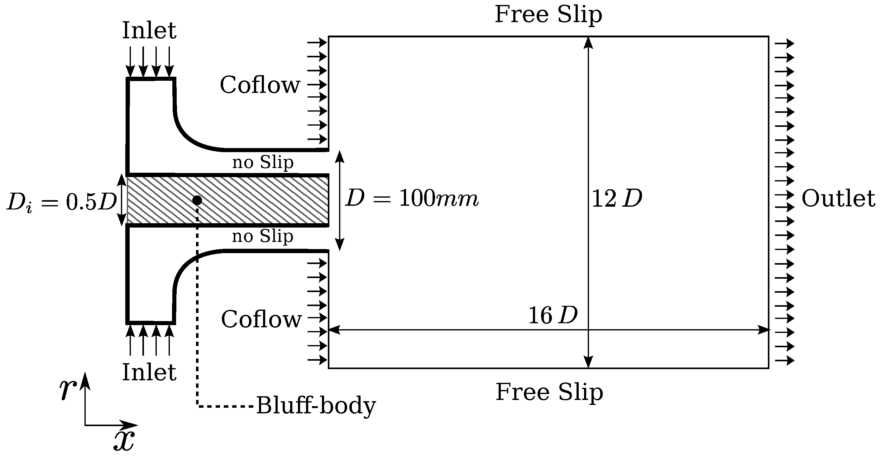
3.1. Flow Configuration

The case studied in this paper corresponds to a turbulent unconfined annular swirling jet discharging into an ambient of the same fluid. The annular jet has an external diameter $D=100\mathrm{mm}$, an internal to external diameter ratio $D_i/D=0.5$ (Figure 1), an inlet Reynolds number $Re=$ 81,500 and a swirl number $S_n=0.9$ in the jet discharge zone, giving an inlet velocity $\begin{array}{c}\hfill U_b=25.5\mathrm{m}/\mathrm{s}\end{array}$. This flow configuration was previously studied through experimental LDA measurements [30,31] and CFD simulations using a LES turbulence model [32]. The results from these studies provide mean and rms velocity data in the near-field region of the jet at different axial positions.

3.2. Computational Domain

The computational domain is three-dimensional and is based on the one used by García-Villalba et al. [32], which is represented in Figure 1. The domain has two main sections: the inlet duct geometry and the discharge zone. In the experimental configuration of Büchner and Petsch [30], the swirl is generated upstream with a swirl generating device composed of adjustable angle vanes. In the numerical simulations the inlet duct is simplified and the geometries of the vanes and the swirl generator are not constructed. This simplification was proposed by García-Villalba et al. [43] to provide a realistic inflow condition for LES simulations of turbulent swirling jets, while keeping the simulation costs low. The discharge zone is extended 12D in the radial direction and 16D in the axial direction to minimize the interference of the boundaries. The outer region of the discharge zone is characterized by a co-flow inlet. The co-flow was not present in the experimental configuration but it was used by García-Villalba et al. [32] to prevent the formation of an unphysical recirculation zone in the outer region of the jet. The fluid introduced in the co-flow inlet has 5% of the bulk velocity $U_b$ in the discharge zone.

3.3. Boundary Conditions

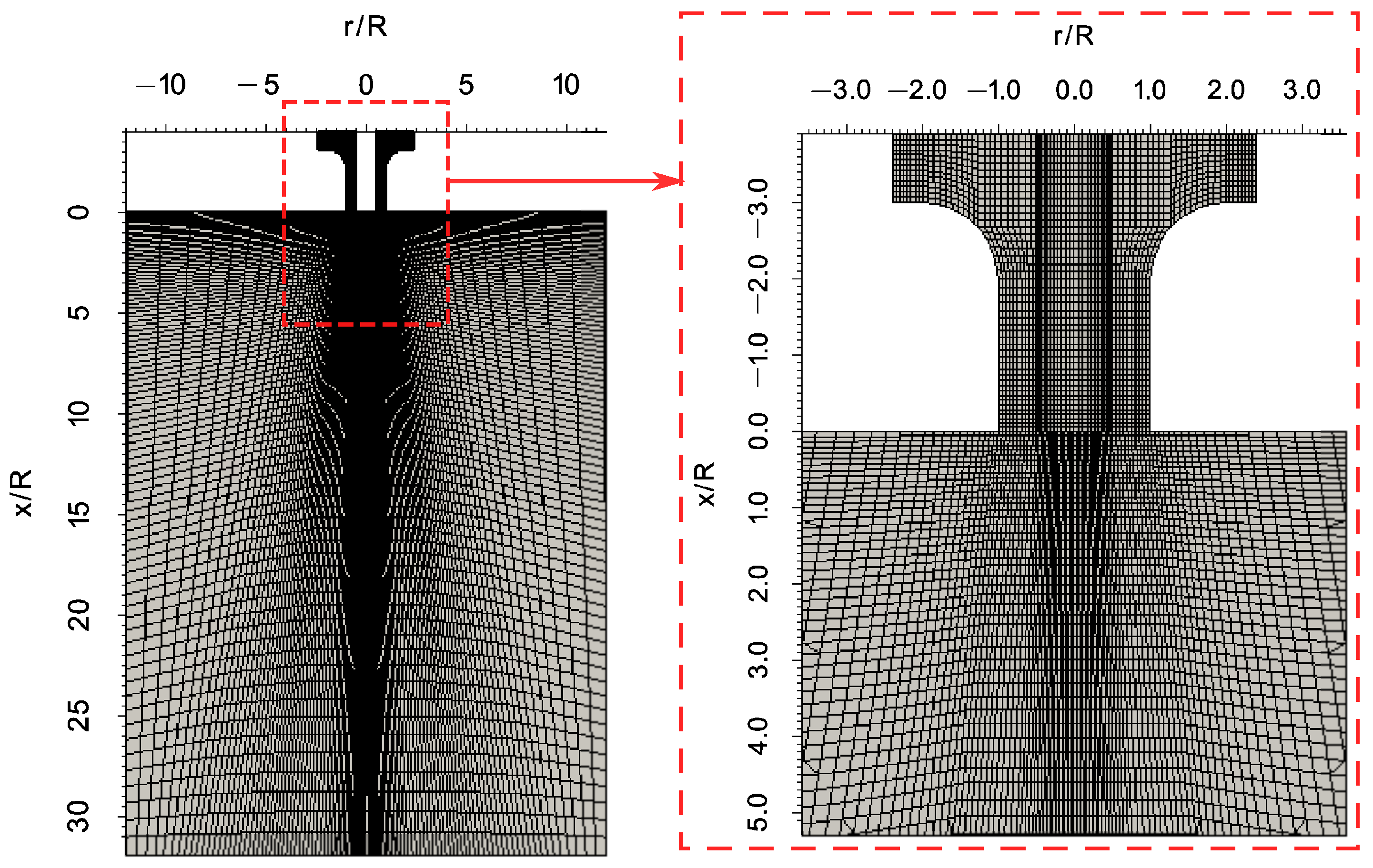
At the inlet boundary (Figure 1), the velocity is prescribed through a fixed-value vector in cylindrical coordinates. This vector is defined in terms of axial, tangential and radial velocity components $(U_x,U_{\theta },U_r)$. The value of the tangential velocity $U_{\theta }$ is adjusted to produce a swirl number $S_n=0.9$ in the jet discharge. $S_n$ is computed in a dimensionless manner:

$$S_n=\frac{\int {}_0^R\rho U_x{U}_{\theta }{r}^{2}dr}{R{\int }_0^R\rho U_x^{2}rdr}.$$

(18)

Here, $S_n$ represents a balance of the product of the axial and tangential momentum $\rho U_x{U}_{\theta }$ of the flow and the axial momentum $\rho U_x^2$. Turbulent variables k($m^2/s^3$) and $\omega$ ($1/s$) are defined in the inlet through a fixed-value condition. Although the initial value set for both k and $\omega$ is very low ($1\times {10}^{-6})$, it does not affect the numerical solution as the correct amount of turbulence is developed through the simplified inlet duct [43]. For the co-flow, the velocity is defined through a Dirichlet type boundary condition (B-C), providing a fixed velocity value that is normal to the boundary. For the inlet duct walls, no-slip conditions are applied, making $U_{x,\theta ,r}=0$ in the walls. Turbulence variables k and $\omega$ are defined in this zone through standard wall functions. The other walls of the domain (discharge zone) are defined with a free-slip condition. For the outlet, a zero-gradient boundary condition is applied to the velocity and turbulence variables. The pressure in the outlet is defined through a fixed-value B-C, with $p_{\mathrm{outlet}}=0.$

3.4. Grid

Two structured grids (one coarse and one fine) were used in the present work. Figure 2 presents general and detailed views of the coarse grid. In both grids the elements are radially and axially concentrated around the jet discharge zone. A positive grow factor was implemented from this point towards the radial boundaries and the outlet. At the inlet duct, the size of the first element from the wall was adjusted to maintain $y^{+}\approx 300$, which represents the upper limit of operation for the use of wall functions. However, no explicit refinement is performed in these zones. Both grids are much coarser than the one used by García-Villalba et al. [32], having from 22 to 6 times less elements. The distribution of the elements in each direction (axial, transversal and radial) for each discretization is presented in

Table 1. Total and direction-wise number of elements in the cylindrical section of the domain for the coarse and fine grids. The element count does not include the section of the inlet diffuser duct.

		Direction
Grid	Elements	$\mathit{x}$	$\mathbf{\theta }$	$\mathit{r}$
Coarse	278,000	90	60	45
Fine	1,000,000	144	88	72

.

For a practical implementation of the current grid in the spray drying simulation, it is expected that the extrapolation of the present arrangement to a spray drying chamber geometry will require from two to three times more grid elements. For the coarse grid, the resulting number of elements is comparable to the one reported by many RANS-based studies of spray dryers (e.g., [44,45,46]). For the fine grid, the resulting number would be similar to the one reported by a recent SAS-based study [47], which is still lower than the one used in a LES study (see Jongsma et al. [16]).

4. Study Cases and Methodology

The main characteristics of the study cases are presented in

Table 2. Study cases for the general configuration presented in Figure 1. The details of the coarse and fine grids are presented in Table 1 and in Figure 2. DES, DDES and SAS turbulence models are used in both grids.

Grid	Coarse			Fine
Case name	1c	2c	3c	1f	2f	3f
Turbulence (SST)	DES	DDES	SAS	DES	DDES	SAS
Courant number (max.)	${\mathrm{Co}}_{\max }=2.5$			${\mathrm{Co}}_{\max }=1.0$
Swirl number	$S_n=0.90\pm 1.5\%$
Bulk velocity	$U_b=25.5\mathrm{m}/\mathrm{s}$

. For each grid, DES, DDES and SAS turbulence models are used, all of them based on the $k-\omega$ SST model. In each case, the swirl number in the jet discharge was calculated using Equation (18) with the sampling data of axial and tangential velocity in the jet discharge zone $(x/R=0)$. The calculated $S_n$ value was calibrated to $S_n=0.90\pm 1.5\%$ by varying the tangential velocity $U_{\theta }$ at the inlet diffuser boundary. It was found that in order to keep $S_n$ within the allowed range, different values of tangential velocity had to be set in the inlet boundary for each grid and turbulence model configuration. The time-step was set in terms of the Courant number due to stability concerns in the solution. Although the backward scheme used for the time interpolation is implicit, its boundedness is not guaranteed and unphysical oscillations may appear in the domain [48]. Preliminary runs were performed to establish the effects of varying the maximum Courant number (${\mathrm{Co}}_{\max }$), which are presented in Figure 3. These results are obtained by adjusting the PIMPLE algorithm to calculate the turbulent properties in each outer loop (pressure-momentum coupling). The use of this setting prevents the calculation of the turbulence fields from being postponed until the last iteration, which would cause an artificially large increase of the simulated rms velocity values, depending on higher values for ${\mathrm{Co}}_{\max }$. In Figure 3 it is detected that the increase of ${\mathrm{Co}}_{\max }$ generates stronger fluctuations in the axial jet discharge zone ($x/R=0.2$), especially in the inner recirculation radial zone ($r/R\lesssim 0.5$). These effects can be explained by a high sensitivity of ${\mathrm{Co}}_{\max }$ on rms velocity as a function of grid resolution, which are comparatively attenuated when using a coarser grid. At lower axial positions (e.g., $x/R=3.0$), most of these artificial fluctuations dissipate quickly, resulting in small differences between the presented ${\mathrm{Co}}_{\max }$ values. Further increases in ${\mathrm{Co}}_{\max }$ values led to much stronger fluctuations at the jet discharge and excessive dissipation downstream. Comparable results are reported by Kalaushina et al. [49] in a LES simulation of a round jet. According to this analysis, the maximum values allowed in the present study are established for the coarse-grid (${\mathrm{Co}}_{\max }=2.5$) and fine-grid (${\mathrm{Co}}_{\max }=1.0$) cases, which allow simulations to be run in appropriate ranges simultaneously for accuracy, numerical stability and speed of solution, as presented in Section 5.

All the study cases were initialized using a steady-state RANS solution with the standard $k-\omega$ SST turbulence model. The running times of the unsteady simulations were defined in terms of a characteristic time $t_b=R/U_b$. First, the case was run for $150t_b$ to allow a complete development of the unsteady flow structures. The sampling of data was initiated at $150t_b$ and ended at $300t_b$. Preliminary simulations carried out during this study indicated that this sampling time was long enough to collect statistically significant velocity data, in agreement with García-Villalba et al. [32]. The instantaneous value of all velocity components ($U_x,U_{\theta },U_r$) was sampled at a frequency of 1000 Hz, using a total of 600 probes. Although the simulation used a variable time-step (in order to maintain the value given to ${\mathrm{Co}}_{\max }$), the reading of the velocity data at the defined sampling frequency was prioritized. The probes were distributed in the domain as follows (Figure 2): 150 probes to sample the jet discharge zone ($x/R=0$) along the annular inlet $(r/R=0.5$ to $r/R=1.0)$ and 150 probes to sample each of the axial positions $x/R=(0.2,1.0,3.0)$ distributed radially from $r/R=0$ to $r/R=4.0$. To obtain the profiles, the sampled data from $150t_b$ to $300t_b$ was averaged in time for each probe position.

5. Results and Discussion

All the study cases were run in a Core i7-7700 desktop using the 4 available physical cores. With the coarse grid and the DES model, the running time was 0.066 h per $t_b$. The use of the DDES model increased the running time by 10%, whereas the SAS model decreased it by 4%. With the fine grid and the DDES model, the cost was increased to 0.64 h per $t_b$. By maintaining ${\mathrm{Co}}_{\max }=1.0$, a very conservative linear extrapolation of these results to the LES grid used by Apte et al. [10] gives 7.84 h per $t_b$, which is around 120 times higher than the cost of the DES in the coarse grid case.

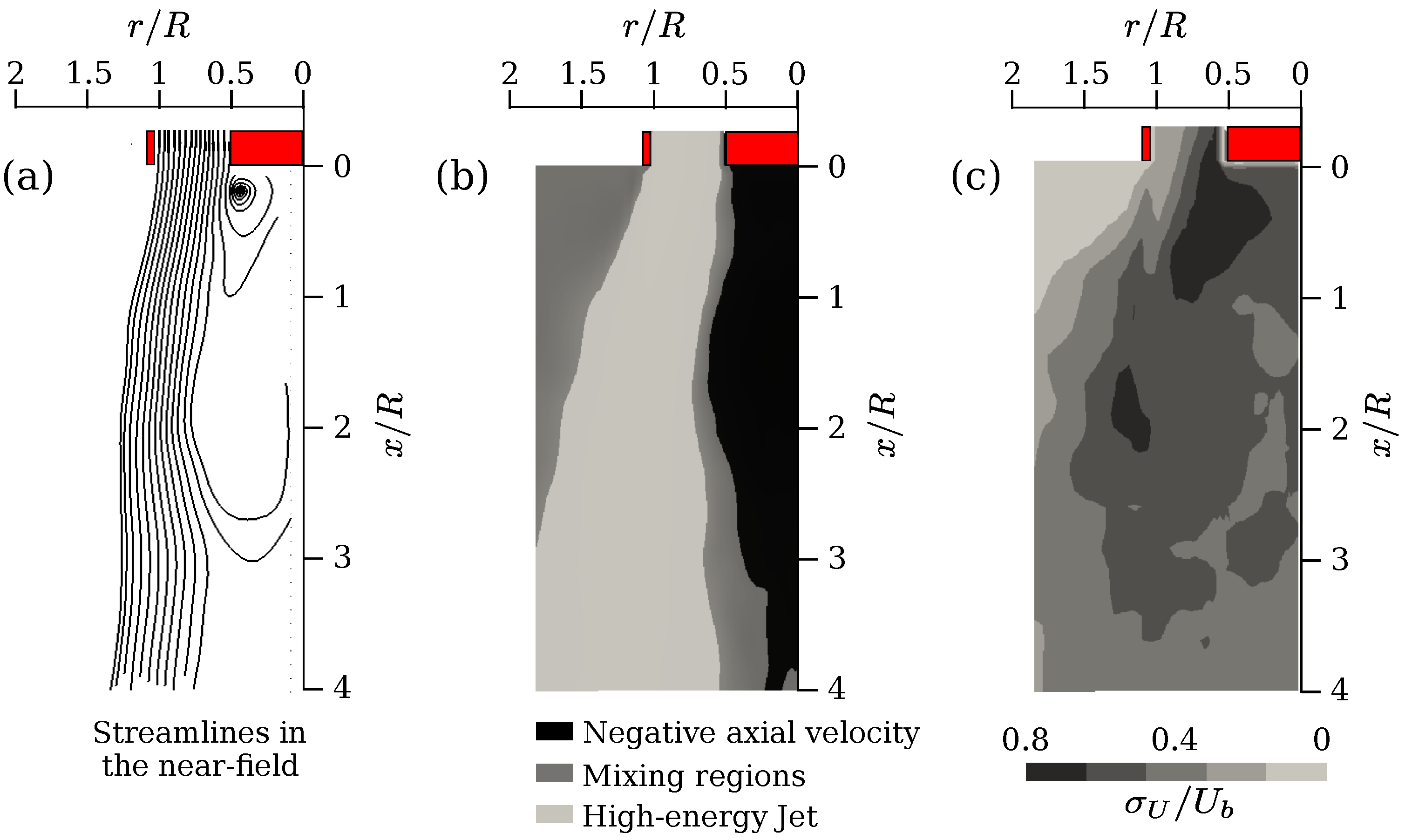
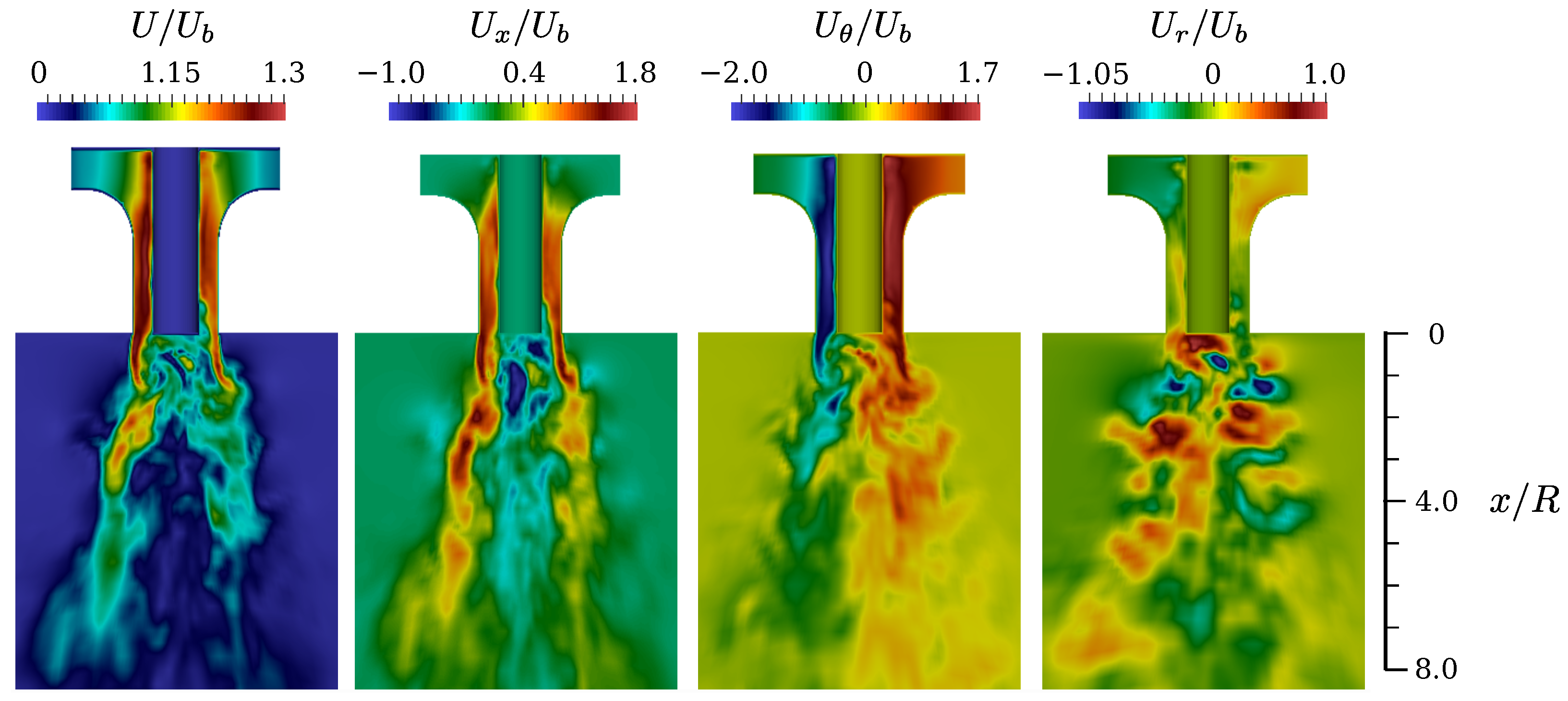
5.1. Description of the Flow Field

The near-field region of the annular jet studied here falls inside a zone defined by Ko and Chan [4] as the initial merging zone. A brief description of this zone using data from a SST-DES simulation (case 1c) is presented next. Results using DDES and SAS models and other grid sizes are similar from a qualitative point of view and are not presented. Figure 4a shows the streamlines of the mean velocity field. The streamlines contain axial and radial velocities and are shown in a 2D symmetry plane. A recirculation zone is observed below the bluff-body (Figure 1) with a maximum radius at $r/R=0.75$ and $x/R=2.0$, and extending downstream beyond $x/R=3.0.$ In co-current spray dryers, the bluff-body accommodates the atomization device. As a result of the recirculation, the streamlines of the high energy jet are displaced radially, delaying the reattachment of the annular flow. The reattachment point is an axial location in the centerline of the jet configuration where the maximum annular velocity is obtained, and marks the start of the decay of the jet. Figure 4b presents some key regions identified in the jet flow in terms of the axial velocity component. The negative axial velocity region ($U_x/U_b<0$) is presented in black and represents the zone where the axial component of the recirculation streamlines has negative values. The inner and outer mixing regions are shown in gray and represent zones with moderate flow velocities ($0.5>U_x/U_b>0$). Both the inner and outer mixing regions are characterized by shear layers caused by the bluff-body (represented in red) and are fundamental in the development of the three-dimensional jet structure as discussed by Danlos et al. [2]. The high-energy jet is shown in light gray and represents the zone with large positive axial velocities $(U_x/U_b>0.5).$ The widening of the high-energy jet region downstream the inlet is caused by shear stresses in the inner and outer mixing regions, which ultimately produce a decay in the jet. Figure 4c shows the standard deviation of the velocity magnitude in the near-field of the jet. The stronger fluctuations are presented just below the bluff-body, in the inner mixing zone and downstream, at $x/R=2.0$ and $r/R=1.25.$ The strength of the fluctuations decreases radially and axially as the inner-recirculation zone weakens. Figure 5 shows the instantaneous velocity fields obtained at $255t_b$. In all velocity components, it is observed that the DES model is capable of resolving large turbulent structures after the flow leaves the duct section. Similar qualitative behaviors were observed through different times $t_{\mathrm{b}}$ with other turbulence models (DDES and SAS). In contrast to the results obtained by García-Villalba et al. [32], resolved turbulent structures inside most of the inlet duct are not differentiated in the radial direction, which is coherent with the coarseness of the grid. Some relevant flow characteristics observed are the following:

• For the axial velocity contours ($U_x/U_b$), the central recirculation region and the high velocity jet are easily differentiated. In this particular case, large-scale detached turbulent structures are detected at $x/R=1.0.$
• For the tangential velocity contours ($U_{\theta }/U_b$), the swirling structure of the jet is clearly noticed. The energy of the swirling flow decays farther from the inlet. Tangential back-flow is also recognized in the outer mixing regions. Differences are also detected in shape and magnitude of the instantaneous tangential flow structures around the symmetry axis.
• For the radial velocity contours ($U_r/U_b$), an alternating behavior of $U_r$ is detected. While little variation on this velocity component is observed inside the inlet diffuser, an alternating pattern in $U_r$ is quickly developed just in the very near-field ($x/R<1.0$).

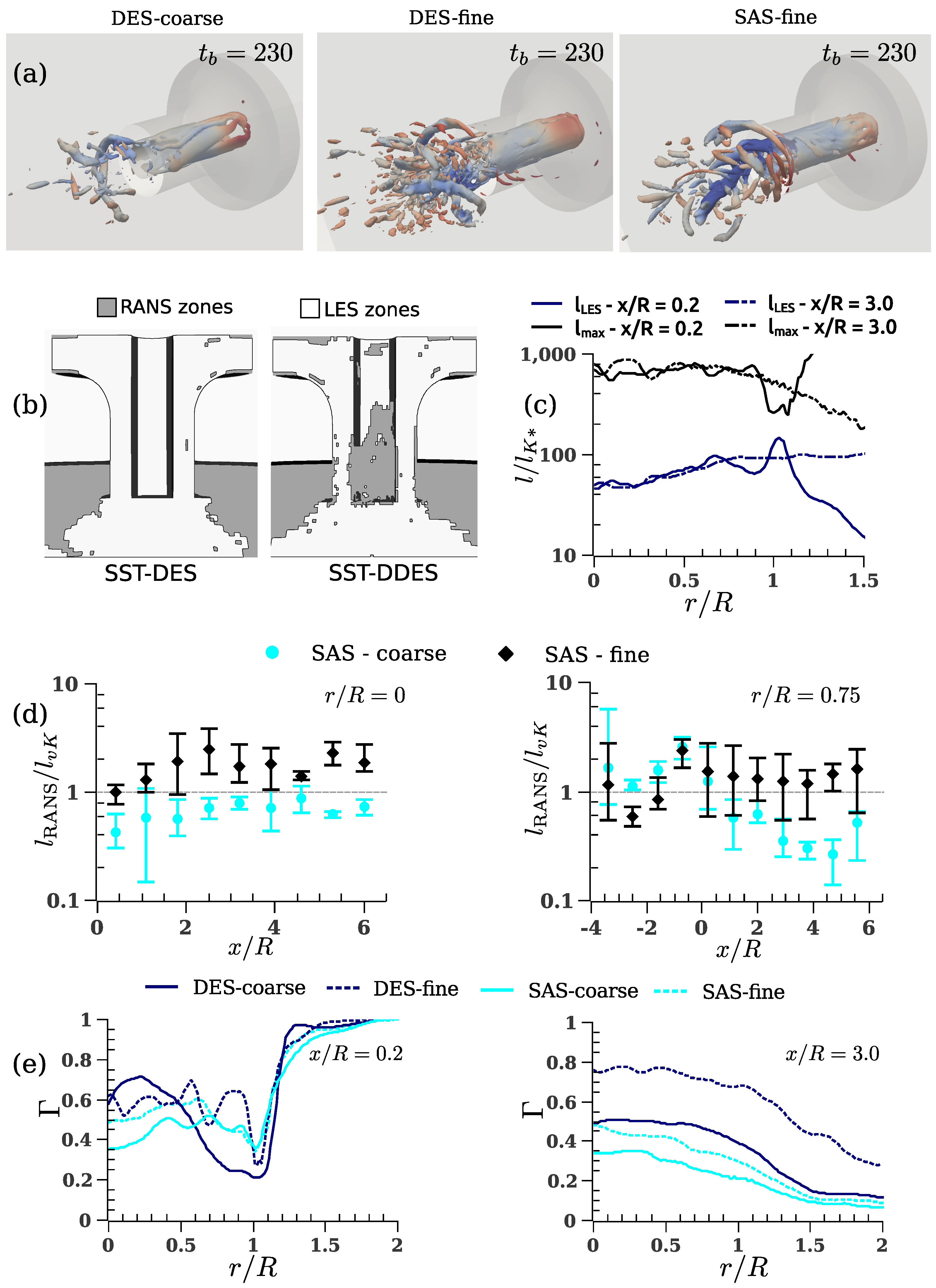
5.2. Grid Size and Turbulence-Resolving Capabilities

Due to the high-coarseness of the grids used, some uncertainties regarding the turbulence-resolving capabilities must be assessed. Therefore, this section presents some quality measures typically evaluated for LES simulations, but also applicable to the DES and SAS models.

Figure 6a shows the coherent structures in the near-field of the jet for cases 1c (DES-coarse), 1f (DES-fine), and 3f (SAS-fine) at $230t_b$. The coherent structures are identified with iso-surfaces of the Q-criterion and colored by the instantaneous pressure value. In comparison with the coarse grid, the fine grid captures a larger number of large-scale vortical flow structures. Using the fine grid, and compared with SAS, the use of DES appears to recreate a greater number of these structures. Figure 6b shows the zonal treatment of DES-based models (cases 1c and 2c) in the near-field of the jet. It is evident that, when DES is used, the first cell from the wall operates mostly in LES mode. In contrast, using DDES, a large proportion of the first cells work in RANS mode, especially before the formation of the inner and outer shear layers. Working in RANS mode near the walls is desirable for DES-based simulations, which allows the use of the robust wall formulation of the $k-\omega$ SST model and a better transfer from modeled (RANS) to resolved (LES) turbulence. This improved behavior of DDES over DES near the wall cannot be generalized. However, in the present case, high sensitivity of the base DES model to the extreme coarseness of the grid was evident.

Figure 6c presents the radial profiles of the ratio of resolved length scales to a pseudo-Kolmogorov length scale $l_{\mathrm{LES}}/l_{K\ast }$ and compares with the $l_{\max }/l_{K\ast }$ ratio. In these relations, the length scale of the resolved eddies $l_{\mathrm{LES}}$ is computed from Equation (9) using the results of case 1f. The length of the largest eddies is estimated as $l_{\max }=k^{3/2}/ϵ$, with $k=k_{\mathrm{LES}}+k_{\mathrm{RANS}}$ and $ϵ$ representing the turbulence dissipation rate, obtained as $ϵ={\beta }^{\ast }k\omega$. The pseudo-Kolmogorov length scale $l_{K\ast }$ represents an approximation obtained using the $ϵ$ value calculated by the turbulence model (case 1f). A better estimation of $l_K$ and $l_{\max }$ is achieved when $ϵ$ is calculated from either DNS or experimental data. However, in the present case, the available experimental data did not provide enough information for its calculation at the presented locations. Everywhere, from $r/R=0$ to $r/R=1.0$, the resolved length $l_{\mathrm{LES}}$ is around two orders of magnitude larger than $l_{K\ast }$, and around 1 order of magnitude shorter than $l_{\max }$. At the high-shear region, around $r/R=1.0$, the ratio of $l_{\mathrm{LES}}/l_{K\ast }$ increases, while $l_{\max }/l_{K\ast }$ decreases. Therefore, in this zone, only a very small portion of the turbulence spectrum is resolved.

Figure 6d presents the axial profiles of the interval-mean ratio of length scales $l_{\mathrm{RANS}}/l_{vK}$ for SAS-bases cases (3c and 3f) at two different radial positions. The modeled length-scale $l_{\mathrm{RANS}}$ is calculated using Equation (6) and the von-Kármán length-scale is calculated using Equation (15). This relation is very important in SAS modeling, as it triggers the operation into eddy-resolving mode and the production of the source term $Q_{\mathrm{SAS}}$ (see Equation (14)). As expected, the use of the fine grid results in larger $l_{\mathrm{RANS}}/l_{vK}$ values. For the coarse grid, the low ratio obtained in some zones, such as the internal recirculation, indicates a RANS-dominant behavior. For the fine grid, and due to the large ranges of $l_{\mathrm{RANS}}/l_{vK}$, some zones alternate between RANS and LES-like operation. This partially explains why in Figure 6a SAS solves a lower number of coherent structures than DES.

Figure 6e shows the radial profiles of the fraction of the resolved turbulent kinetic energy for the DES and SAS cases. The resolved fraction is calculated as $\mathsf{\Gamma }=k_{\mathrm{LES}}/\left(k_{\mathrm{LES}}+k_{\mathrm{RANS}}\right)$. In LES modeling, it is considered that this fraction should be greater than 0.8 [50]. In this study, a lower value of $\mathsf{\Gamma }$ is expected due to the coarseness of the grids. In all cases, the lowest $\mathsf{\Gamma }$ values are observed in the high-shear region near the jet discharge $(r/R=1.0,x/R=0.2)$. In the DES cases, it is evident that in this region $l_{\mathrm{LES}}$ is only slightly larger than $l_{\max }$, as shown in Figure 6b. In lower axial positions, the $\mathsf{\Gamma }$ values are more smoothly distributed, being higher in the jet centerline and decreasing in the radial direction. For DES, the use of a finer grid provides a clear improvement in the turbulence resolution capacity. For SAS, this increase is minor, only improving the results of the DES cases in the high-shear region. These results and those presented in Figure 6a,d indicate that, in the current case configuration, the SAS model evidences some difficulties in working under scale-resolving mode.

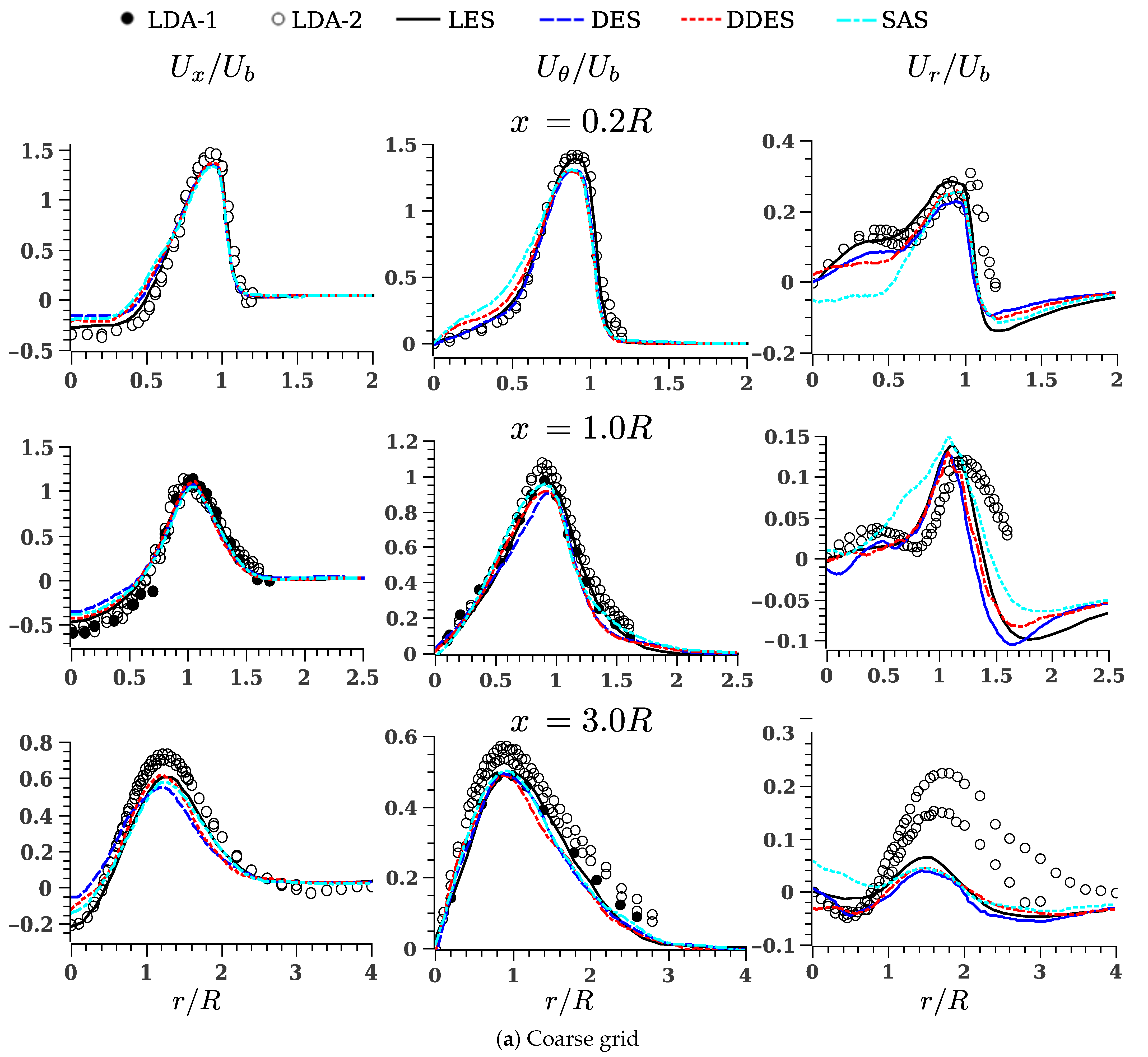
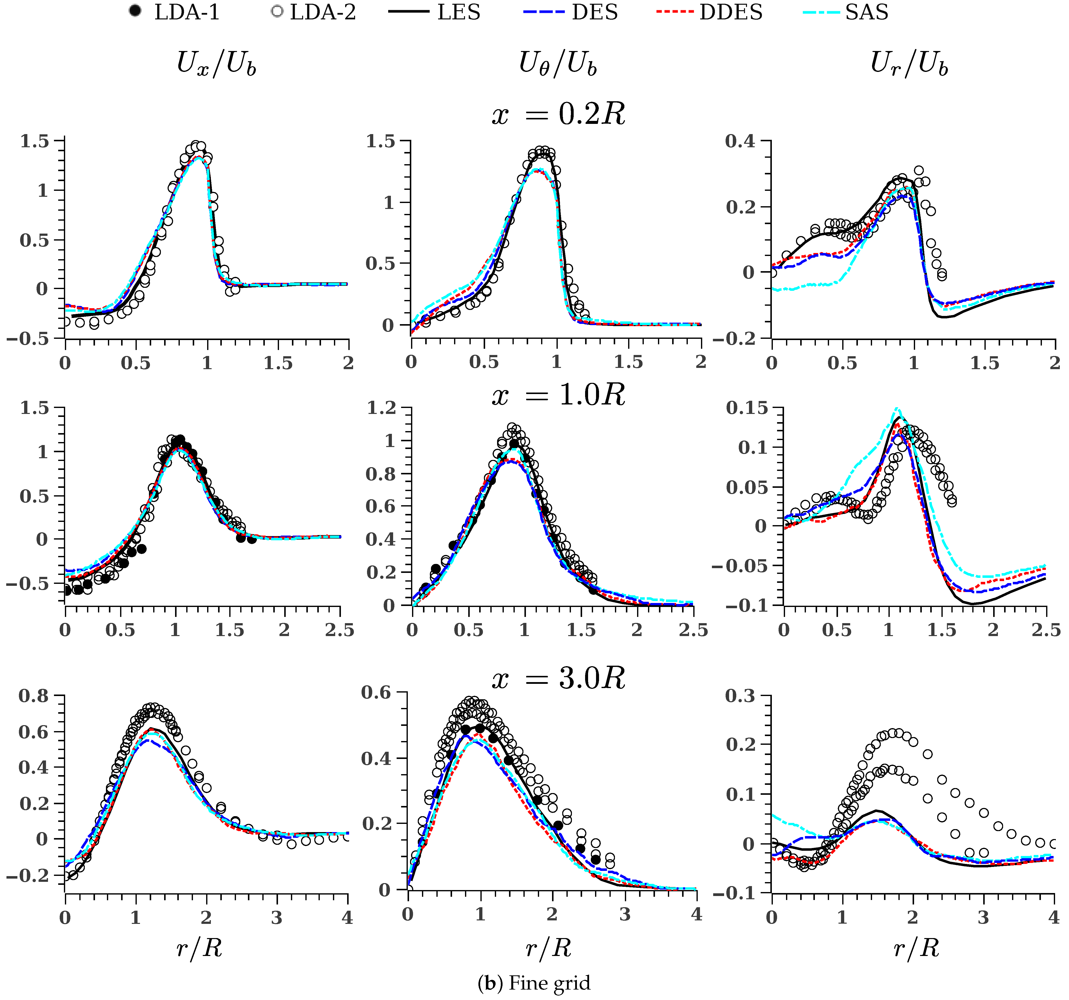
5.3. Mean Velocity Profiles: Comparison with Experimental and LES Data

In spray drying, the airflow pattern in the chamber mainly determines the movement and transport of droplets [51]. As the initial droplet-gas contact occurs in the near-field region of the jet, an accurate prediction of mean velocity profiles of the gas phase in this location is essential. Figure 7a,b present the radial profiles of the mean velocity components at three different axial positions downstream the annular inlet region $(x/R=0.2,1.0,3.0)$ using the DES, DDES and SAS models, with coarse and fine grids. Overall, the DES, DDES and SAS results agree well with LES and experimental data. For the axial velocity $U_x/U_b$, evident differences are observed downstream the inlet ($x/R=1.0,3.0)$ in zones of negative axial velocity (recirculation zones), where SAS and DDES produce better results than DES. This occurs in both coarse and fine grids, although smaller differences with LES data exist when the fine grid is used. The better accuracy of the SAS model over the DES in zones with recirculation has been previously reported by Zheng et al. [52]. The improvement of DDES over DES in this zone is related to the treatment that DDES gives to the cells close to walls boundaries, which was presented in Figure 6b. This results in a better representation of the inner recirculation zone. Other differences in the results of the axial velocity $U_x$ are seen in the jet decay, specially at $x/R=3.0$. In this location, for both grids and using the DES model, the jet shape is more flattened than using DDES or SAS.

For the tangential velocity $U_{\theta }/U_b$, the differences between the models are very small and only noticeable in the inner shear layer near the inlet ($x/R=0.2$, $r/R=0.5$), where DDES and SAS produce inferior results than DES. This difference is smaller if the fine grid is used. For the radial velocity $U_r/U_b$, in the very near field ($x/R=0.2,1.0)$ and for both grids, DES and DDES curves match closely with LES data, while the SAS results differ significantly. At $x/R=3.0$, large differences between experimental data and all CFD results are detected. Although the presence of experimental errors in this location measurements is not discarded [32], DES, DDES and to a lesser degree SAS results at $x/R=3.0$ closely follow the LES trend.

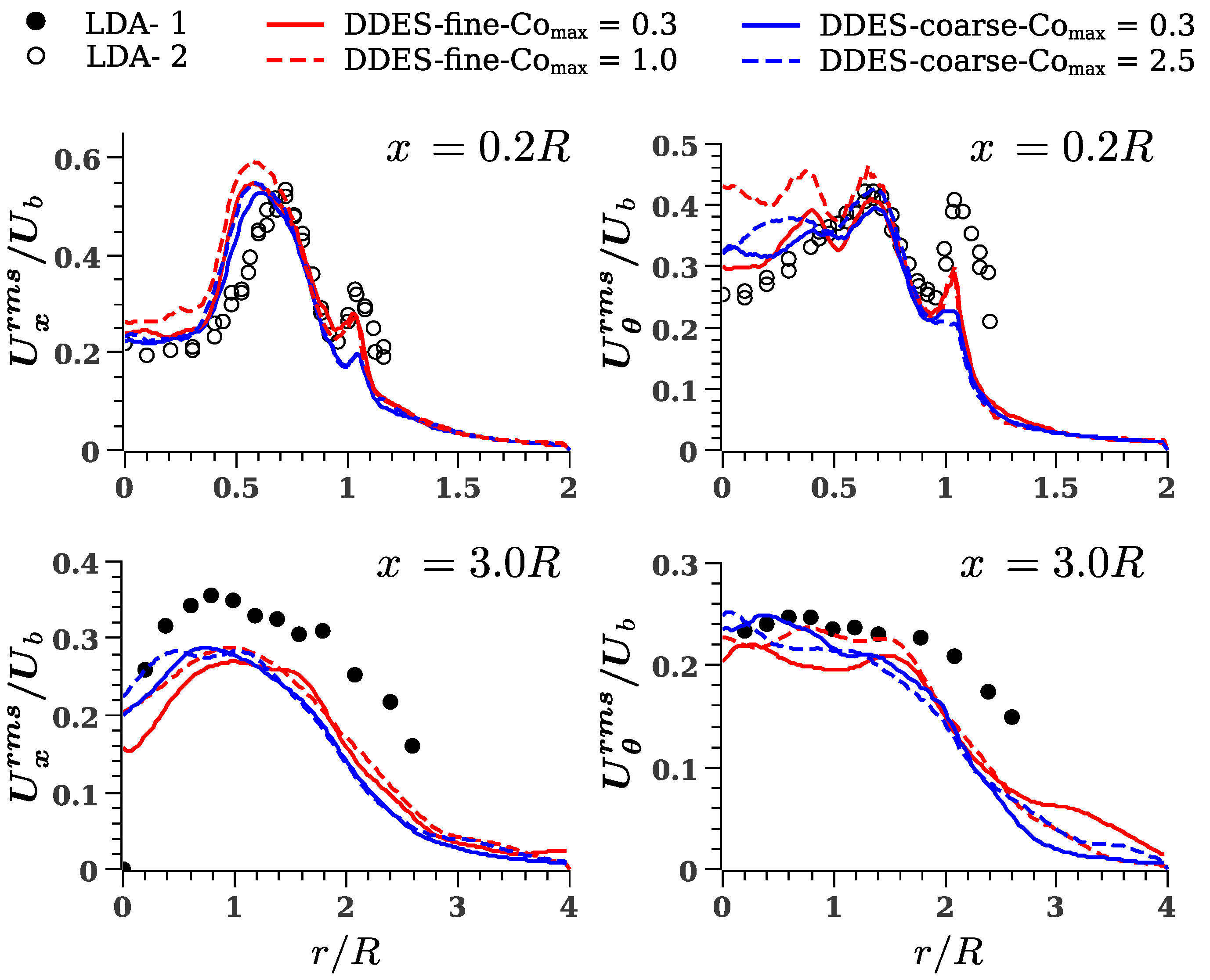
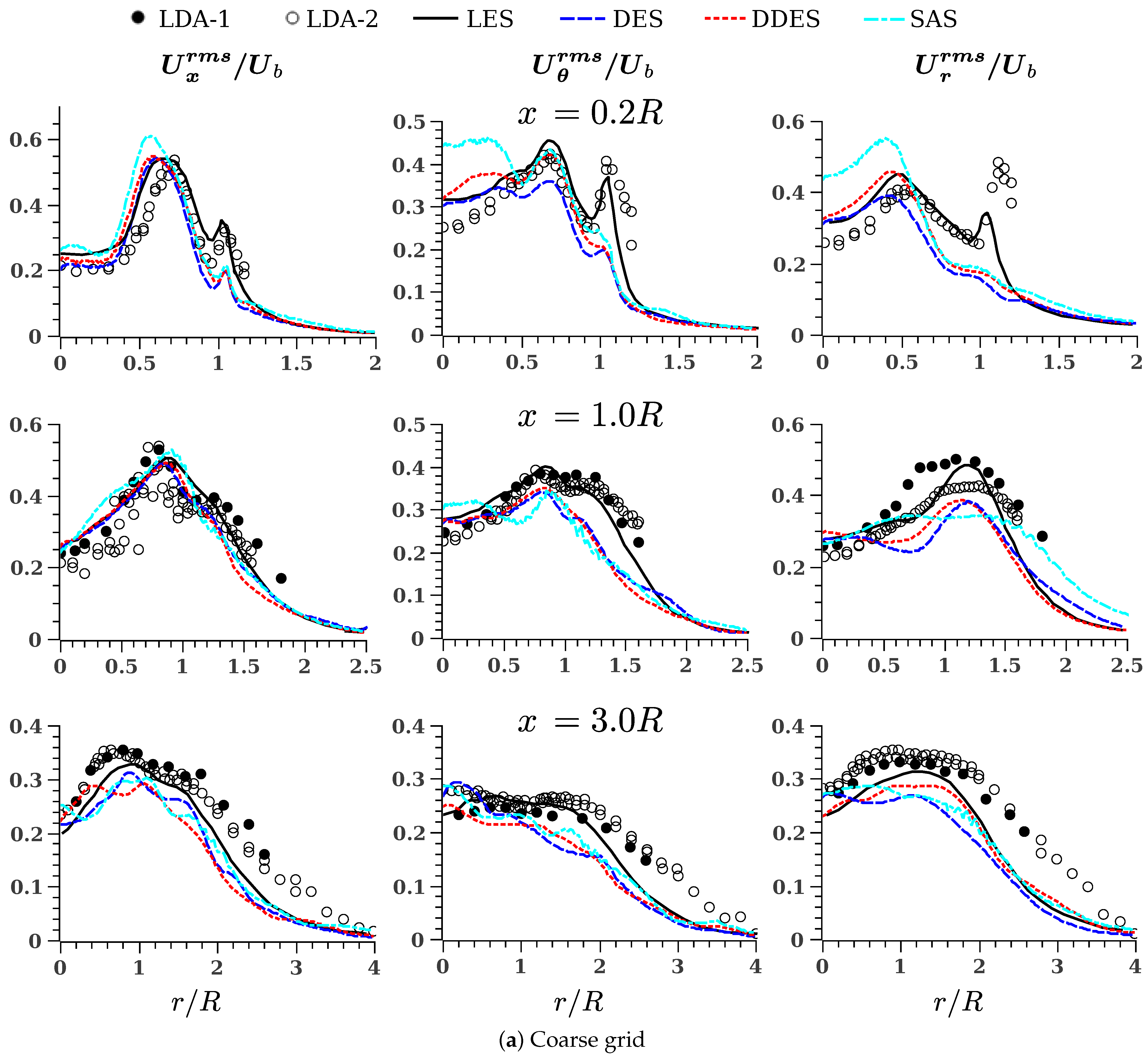
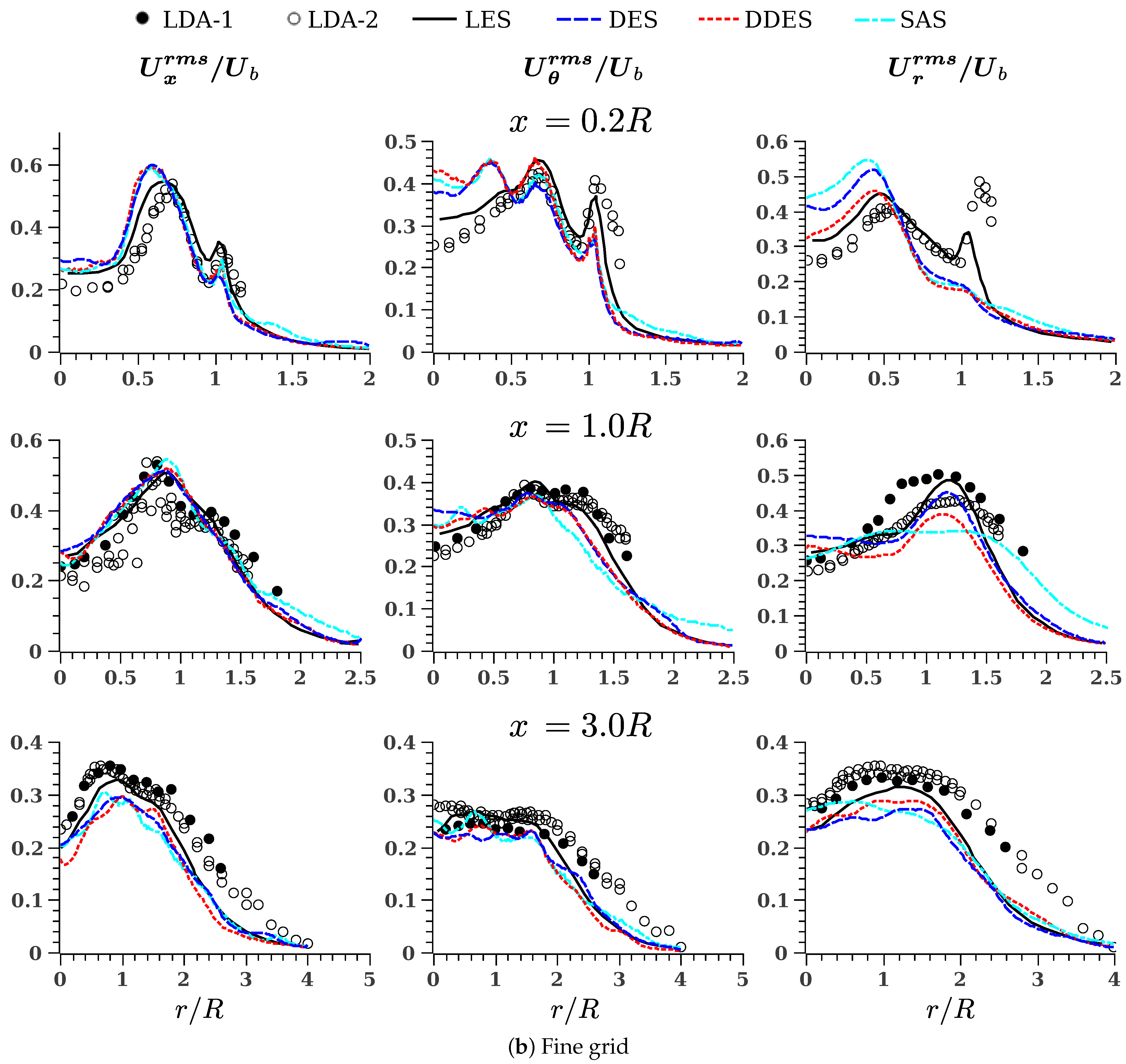
5.4. Fluctuations: Comparison with Experimental and LES Data

Figure 8a,b presents the radial profiles of rms fluctuations of velocity components ($x,\theta ,r$) for the same study case and using the coarse and fine grids. The rms value gives a good indication of the unsteady behavior of the jet. It is crucial in spray drying as it governs the turbulent dispersion of droplets. Overall, for the axial and tangential velocities ($U_x,U_{\theta })$, DES, DDES and SAS data trends are similar to LES and LDA, especially in lower axial positions ($x/R=1.0,3.0),$ where all the three models perform remarkably well for both grids. Significant differences with LES and LDA data are observed mainly in two zones. First, in the very near-field of the jet, at $x/R=0.2$, for all turbulence models, the fine grid overpredicts the rms values in the inner recirculation region ($r/R=0$ to $0.5$). In this zone the coarse grid brings better results for DES and DDES. For the SAS model, both grid sizes overpredict in a similar way the rms values. Second, in the outer shear layer located at $x/R=0.2$ and $r/R=1.0$, DES, DDES and SAS do not reproduce well the narrow peak shown by the LDA and LES data, especially if the coarse grid is used. This is explained in the decrease of the resolved fraction of turbulent kinetic energy $\mathsf{\Gamma }$ due to the coarseness of the grids, as presented in Figure 6e.

5.5. Quantitative Differences: Error Calculation

5.5.1. Error Criteria

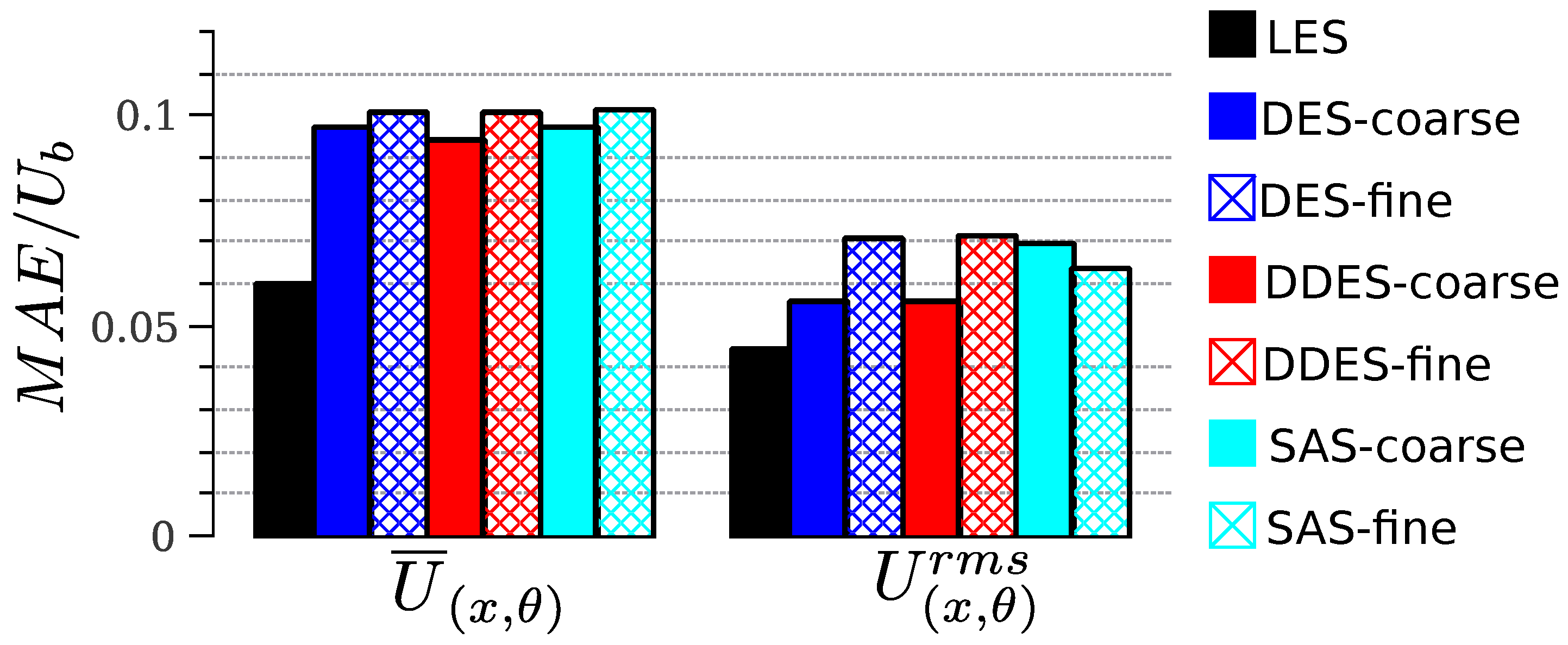
The qualitative differences between the DES, DDES and SAS data for the mean and rms velocity profiles are very small, thus limiting the discussion of the results. To provide a quantitative assessment, a mean absolute error criteria (MAE) is used. The MAE is defined as:

$$MAE=\frac{1}{n}\sum _{i=1}^n\left|U_i^s-U_i^m\right|,$$

(19)

where $n=150$ represents the number of probes in the radial direction. For every radial position i, there is a simulated quantity $U_i^s$ and a measured quantity $U_i^m$. The measured quantity is obtained by interpolating the LDA measurements from Büchner and Petsch [30] (labeled as LDA-2) to match the CFD data sampled along the radial direction. The results from Hillemanns [31] (labeled as LDA-1), are not used since those values are not available for some radial and axial positions. The measurements of the radial component of the velocity $U_r$ were not used, as they lack reliability at $x/R=3.0$. The use of other error indicators such as the relative error $e_r=\left|\frac{U_i^s-U_i^m}{U_i^m}\right|$ was not feasible, as many points presented a velocity value close to zero, which resulted in very large error values.

5.5.2. Global MAE

The results of the application of the MAE criteria are presented in Figure 9. The quantities evaluated are the mean velocity $U_{\left(x,\theta \right)}$ and the rms fluctuations $U_{\left(x,\theta \right)}^{rms}.$ For $U_{\left(x,\theta \right)}$, the MAE obtained from DES, DDES and SAS is almost twice than with LES, and the effects of using the coarse and fine grids are very small. For $U_{(x,\theta )}^{rms}$, the differences with LES results are smaller and the effects of the grid size are more appreciable. For DES and DDES models, using the coarse grid produces lower MAE values than the ones achieved with the fine grid. This is explained in the contribution of the unphysical fluctations at the jet discharge as a function of higher ${\mathrm{Co}}_{\max }$ values. In addition, due to the very small number of elements used in the coarse grid, some regions may be constantly switching between LES and RANS modes, therefore, providing insufficient LES content or delaying its generation and thus decreasing the rms values. These considerations do not affect the SAS model in the same way, since its LES content is not activated directly by the grid spacing. Consequently, when the SAS model is used, the fine grid achieves a lower MAE $U_{(x,\theta )}^{rms}$ than the coarse grid.

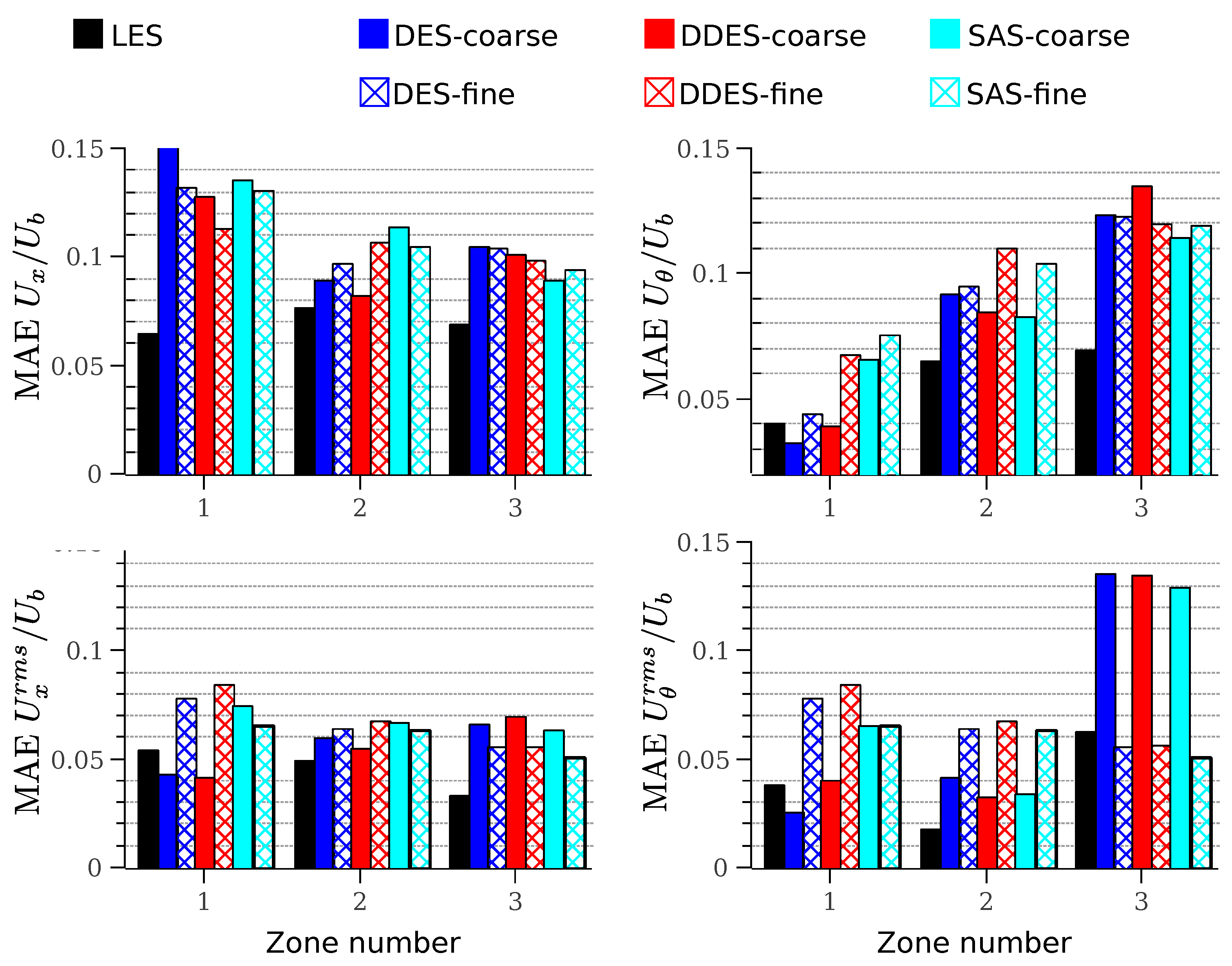
5.5.3. MAE per Jet Zones

The global MAE results bring important quantitative information regarding the overall performance of the different turbulence models and CFD cases. However, it falls short to explain specific performance in different regions of the jet. Figure 10 presents a region-based MAE comparing different turbulence models and grid sizes. Three zones are considered: the zone 1 or axial recirculation region with $U_x<0$; the zone 2 or high-energy jet region, covering from $x/R=0$ to $1.0$ and $U_x>0$, and the zone 3 or outer jet, from $x/R=1.0$ to the maximum measured radial position.

For the coarse grid, with the exception of the axial velocity MAE, in the inner recirculation zone (zone 1), the behavior of DES and DDES models is very good, with lower MAE values than the ones obtained using LES. In the high-energy region of the jet (zone 2), the DDES model produces the lowest MAE among all the studied cases, which is very close to the values predicted by the LES model. In the outer jet (zone 3), the behavior of SAS is better by a small margin than those of DES and DDES. The effect of the grid on the MAE depends on the zone. For DES and DDES models in zones 1 and 2, where the local Courant number is large, the fine grid case tends to generate higher MAE values of $U^{rms}$. In contrast, in the outer jet (zone 3) and for all turbulence formulations, using the fine grid has a marked effect decreasing the MAE of $U_{\theta }^{rms}$. This is partially explained by the structured nature of the grid. As the jet expands radially, the tangential distance between the grid elements increases and the grid-induced errors become larger in high-shear regions. For the SAS model, the effects of the grid on the MAE per zone cannot be generalized, and only become significant in the prediction of the rms fluctuations of the tangential velocity $U_{\theta }$ at zone 3.

6. Conclusions

This paper presents DES, DDES and SAS computations in the near-field of a swirling annular jet. The computations were performed with a low-cost approach; therefore, very coarse grids were used. A detailed comparison of the numerical results with the available LES and LDA data was performed to assess the turbulence-resolving capabilities of the eddy-resolving methods used. The results of the comparison show the cost-effectiveness of the evaluated modeling approach and its applicability to the simulation of spray drying processing and other industrial applications featuring annular-swirling inlets.

From a general perspective, considering the coarseness of the grids used, all three models performed reasonably well. In all cases, the predicted mean-flow properties and first-order turbulent statistics agreed well with experimental and LES data. Although differences in the predictions from the three models are minor, these must be taken into account as they may become larger and more significant in the far-field. Overall, the DDES model produces the best results. In comparison with the DES model, DDES switches to RANS mode much more often in the proximity of walls; therefore, it uses a correct wall-modeling formulation, which results in a better energy transfer from modeled to resolved scales. This should be more significant in more complex applications, such as spray drying, where the predicted decay on the far-field of the jet and the recirculating flow near the walls might suffer from an inappropriate near-wall formulation. Due to the importance of wall-modeling and switching between RANS and LES operation, a future evaluation of the improved DDES model (IDDES) proposed by [36] is relevant, particularly due to its improved LES/RANS blending behavior near the walls and in the so-called “gray zones” of the DES method.

Regarding the SAS model, it achieved good results in the prediction of mean-flow velocities. However, it presented some difficulties in accurately predicting first-order turbulent statistics, especially when using the coarsest grid. Similar issues in the prediction of turbulence statistics in a coarse grid with low inlet turbulence have been reported by Zheng et al. [52]. In addition, it was observed that SAS resolved a lower portion of the turbulence spectrum than DES-based models. In other study cases, and using finer grids, the SAS model has been known to perform similarly to LES, but in the actual flow configuration it seems that the coarseness of the grids and the insufficient turbulence production in the inlet duct are affecting its operation under scale-resolving mode.

The results of this study provide evidence on the ability of DES to tolerate coarse grids when modeling industrial flows, in agreement with Gimbun et al. [53]. They also indicate that, when very coarse grids are used under large Courant number conditions, the improvement obtained through grid refinement is limited to some turbulence statistics, being more marked in certain regions of the domain. Some of these regions were identified in Figure 6, as well as in the error analysis, and include the outer shear layer and the inner recirculation zone (among others). This information is fundamental to incorporating an adaptive mesh refinement (AMR) method, by directing the refinement efforts towards the grid elements located in these key zones. For the SAS model, the improvement obtained from the refinement was similar for most flow regions.

When implemented in simulations of spray drying processes with swirling inflow conditions, the cost-effective approach used in this study will be capable of accurately resolving a significant portion of the turbulence downstream of the jet discharge, which represents a critical region for the process. As a result, compared with standard URANS approaches using the same grid, an improved prediction of particle motion is expected. The degree of improvement will depend on, among other factors, the portion of the turbulence being resolved, for which a very coarse grid is lower than for a well-resolved LES. Further work under development will extend this analysis to evaluate the particle dispersion capabilities in a similar flow problem [10,54] using the same low-cost approach adopted in this investigation. This research can be continued in industrial simulations of other similar flow problems such as two-phase pressure-swirl atomizers [55].

References

1. Chterev, I.; Foley, C.; Foti, D.; Kostka, S.; Caswell, A.; Jiang, N.; Lynch, A.; Noble, D.; Menon, S.; Seitzman, J.; et al. Flame and flow topologies in an annular swirling flow. Combust. Sci. Technol. 2014, 186, 1041–1074. [Google Scholar] [CrossRef]
2. Danlos, A.; Lalizel, G.; Patte-Rouland, B. Experimental characterization of the initial zone of an annular jet with a very large diameter ratio. Exp. Fluids 2013, 54, 1–17. [Google Scholar] [CrossRef] [Green Version]
3. García-Villalba, M.; Fröhlich, J. LES of a free annular swirling jet–Dependence of coherent structures on a pilot jet and the level of swirl. Int. J. Heat Fluid Flow 2006, 27, 911–923. [Google Scholar] [CrossRef]
4. Ko, N.; Chan, W. Similarity in the initial region of annular jets: Three configurations. J. Fluid Mech. 1978, 84, 641–656. [Google Scholar] [CrossRef]
5. Langrish, T.; Williams, J.; Fletcher, D. Simulation of the effects of inlet swirl on gas flow patterns in a pilot-scale spray dryer. Chem. Eng. Res. Des. 2004, 82, 821–833. [Google Scholar] [CrossRef]
6. Masters, K. Spray Drying Handbook; Longman Scientific & Technical: Harlow, UK, 1991; ISBN 9780470217436. [Google Scholar]
7. Lampa, A.; Fritsching, U. Large Eddy Simulation of the spray formation in confinements. Int. J. Heat Fluid Flow 2013, 43, 26–34. [Google Scholar] [CrossRef]
8. Gicquel, L.Y.; Staffelbach, G.; Poinsot, T. Large eddy simulations of gaseous flames in gas turbine combustion chambers. Prog. Energy Combust. Sci. 2012, 38, 782–817. [Google Scholar] [CrossRef] [Green Version]
9. Pitsch, H. Large-eddy simulation of turbulent combustion. Annu. Rev. Fluid Mech. 2006, 38, 453–482. [Google Scholar] [CrossRef] [Green Version]
10. Apte, S.V.; Mahesh, K.; Moin, P.; Oefelein, J.C. Large-eddy simulation of swirling particle-laden flows in a coaxial-jet combustor. Int. J. Multiph. Flow 2003, 29, 1311–1331. [Google Scholar] [CrossRef]
11. Jakirlic, S.; Hanjalic, K.; Tropea, C. Modeling rotating and swirling turbulent flows: A perpetual challenge. AIAA J. 2002, 40, 1984–1996. [Google Scholar] [CrossRef]
12. Lampa, A.; Fritsching, U. Analysis of confined spray processes for powder production. In Proceedings of the ICLASS 2012 12th Triennial International Conference on Liquid Atomization and Spray Systems, Heidelberg, Germany, 2–6 September 2012. [Google Scholar]
13. Fletcher, D.; Langrish, T. Scale-adaptive simulation (SAS) modelling of a pilot-scale spray dryer. Chem. Eng. Res. Des. 2009, 87, 1371–1378. [Google Scholar] [CrossRef]
14. Francia, V.; Martín, L.; Bayly, A.; Simmons, M. Deposition and wear of deposits in swirl spray dryers: The equilibrium exchange rate and the wall-borne residence time. Procedia Eng. 2015, 102, 831–840. [Google Scholar] [CrossRef] [Green Version]
15. Kieviet, F.; Van Raaij, J.; De Moor, P.; Kerkhof, P. Measurement and modelling of the air flow pattern in a pilot-plant spray dryer. Chem. Eng. Res. Des. 1997, 75, 321–328. [Google Scholar] [CrossRef] [Green Version]
16. Jongsma, F.; Innings, F.; Olsson, M.; Carlsson, F. Large eddy simulation of unsteady turbulent flow in a semi-industrial size spray dryer. Dairy Sci. Technol. 2013, 93, 373–386. [Google Scholar] [CrossRef] [Green Version]
17. Jasak, H.; Luo, J.; Kaluderčić, B.; Gosman, A.; Echtle, H.; Liang, Z.; Wirbeleit, F.; Wierse, M.; Rips, S.; Werner, A.; et al. Rapid CFD simulation of internal combustion engines. SAE Technical Paper. SAE Trans. 1999, 108, 1694–1703. [Google Scholar] [CrossRef]
18. Fröhlich, J.; von Terzi, D. Hybrid LES/RANS methods for the simulation of turbulent flows. Prog. Aerosp. Sci. 2008, 44, 349–377. [Google Scholar] [CrossRef]
19. Fureby, C. Towards the use of large eddy simulation in engineering. Prog. Aerosp. Sci. 2008, 44, 381–396. [Google Scholar] [CrossRef]
20. Menter, F.; Kuntz, M.; Langtry, R. Ten years of industrial experience with the SST turbulence model. In Proceedings of the 4th International Symposium on Turbulence, Heat and Mass Transfer, Antalya, Turkey, 12–17 October 2003; Volume 4, pp. 625–632. [Google Scholar]
21. Zhiyin, Y. Large-eddy simulation: Past, present and the future. Chin. J. Aeronaut. 2015, 28, 11–24. [Google Scholar] [CrossRef] [Green Version]
22. Javadi, A.; Nilsson, H. A comparative study of scale-adaptive and large-eddy simulations of highly swirling turbulent flow through an abrupt expansion. In IOP Conference Series: Earth and Environmental Science; IOP Publishing: Bristol, UK, 2014; Volume 22, p. 022017. [Google Scholar] [CrossRef] [Green Version]
23. Javadi, A.; Nilsson, H. LES and DES of strongly swirling turbulent flow through a suddenly expanding circular pipe. Comput. Fluids 2015, 107, 301–313. [Google Scholar] [CrossRef]
24. Paik, J.; Sotiropoulos, F. Numerical simulation of strongly swirling turbulent flows through an abrupt expansion. Int. J. Heat Fluid Flow 2010, 31, 390–400. [Google Scholar] [CrossRef]
25. Mansouri, Z.; Boushaki, T. Investigation of large-scale structures of annular swirling jet in a non-premixed burner using delayed detached eddy simulation. Int. J. Heat Fluid Flow 2019, 77, 217–231. [Google Scholar] [CrossRef]
26. Gimbun, J.; Muhammad, N.I.S.; Law, W.P. Unsteady RANS and detached eddy simulation of the multiphase flow in a co-current spray drying. Chin. J. Chem. Eng. 2015, 23, 1421–1428. [Google Scholar] [CrossRef] [Green Version]
27. Noor, M.; Jolius, G. Detached eddy simulation (DES) of co-current spray dryer. Int. J. Technol. Manag. 2013, 2, 17–22. [Google Scholar]
28. Anandharamakrishnan, C. Computational Fluid Dynamics Applications in Food Processing; Springer: New York, NY, USA, 2013. [Google Scholar] [CrossRef]
29. Mujumdar, A.; Huang, L.; Chen, X. An overview of the recent advances in spray-drying. Dairy Sci. Technol. 2010, 90, 211–224. [Google Scholar] [CrossRef] [Green Version]
30. Büchner, H.; Petsch, O. Experimental investigation of instabilities in turbulent premixed flames. In Proceedings of the 1st International Workshop on Unsteady Combustion, Karlsruhe, Germany, 8–9 July 2004. [Google Scholar]
31. Hillemanns, R. Das Strömungs-und Reaktionsfeld sowie Stabilisierungseigenschaften von Drallflammen unter dem Einfluss der inneren Rezirkulationszone. Ph.D. Thesis, Universitaet Karlsruhe, Karlsruhe, Germany, 1988. [Google Scholar]
32. García-Villalba, M.; Fröhlich, J.; Rodi, W. Identification and analysis of coherent structures in the near field of a turbulent unconfined annular swirling jet using large eddy simulation. Phys. Fluids 2006, 18, 055103. [Google Scholar] [CrossRef]
33. Jin, Y.; Chen, X.D. A three-dimensional numerical study of the gas/particle interactions in an industrial-scale spray dryer for milk powder production. Dry. Technol. 2009, 27, 1018–1027. [Google Scholar] [CrossRef]
34. Menter, F. Two-equation eddy-viscosity turbulence models for engineering applications. AIAA J. 1994, 32, 1598–1605. [Google Scholar] [CrossRef] [Green Version]
35. Jubaer, H.; Afshar, S.; Xiao, J.; Chen, X.D.; Selomulya, C.; Woo, M.W. On the effect of turbulence models on CFD simulations of a counter-current spray drying process. Chem. Eng. Res. Des. 2019, 141, 592–607. [Google Scholar] [CrossRef]
36. Travin, A.K.; Shur, M.L.; Spalart, P.R.; Strelets, M.K. Improvement of delayed detached-eddy simulation for LES with wall modelling. In Proceedings of the European Conference on Computational Fluid Dynamics ECCOMAS CFD, Egmond aan Zee, The Netherlands, 5–8 September 2006. [Google Scholar]
37. Strelets, M. Detached eddy simulation of massively separated flows. In Proceedings of the 39th Aerospace Sciences Meeting and Exhibit, Reno, NV, USA, 8–11 January 2001; p. 879. [Google Scholar] [CrossRef]
38. Gritskevich, M.S.; Garbaruk, A.V.; Schütze, J.; Menter, F.R. Development of DDES and IDDES formulations for the k-ω shear stress transport model. Flow Turbul. Combust. 2012, 88, 431–449. [Google Scholar] [CrossRef]
39. Egorov, Y.; Menter, F. Development and application of SST-SAS turbulence model in the DESIDER project. In Advances in Hybrid RANS-LES Modelling; Springer: Berlin/Heidelberg, Germany, 2008; pp. 261–270. [Google Scholar] [CrossRef]
40. Travin, A.; Shur, M.; Strelets, M.; Spalart, P. Physical and numerical upgrades in the detached-eddy simulation of complex turbulent flows. In Advances in LES of Complex Flows; Springer: Berlin/Heidelberg, Germany, 2002; pp. 239–254. [Google Scholar] [CrossRef]
41. Jasak, H. Error analysis and estimation for the finite volume method with applications to fluid flows. Ph.D Thesis, University of London, London, UK, 1996. [Google Scholar]
42. Holzmann, T. Mathematics, Numerics, Derivations and OpenFOAM®, Holzmann CFD. Available online: https://www.researchgate.net/publication/307546712_Mathematics_Numerics_Derivations_and_OpenFOAMR (accessed on 5 September 2021).
43. García-Villalba, M.; Fröhlich, J.; Rodi, W. On inflow boundary conditions for large eddy simulation of turbulent swirling jets. In Proceedings of the 21st Int. Congress of Theoretical and Applied Mechanics, Warsaw, Poland, 15–21 August 2004. [Google Scholar]
44. Anandharamakrishnan, C.; Gimbun, J.; Stapley, A.G.F.; Rielly, C.D. A study of particle histories during spray drying using computational fluid dynamic simulations. Dry. Technol. 2010, 28, 566–576. [Google Scholar] [CrossRef] [Green Version]
45. Keshani, S.; Montazeri, M.H.; Daud, W.R.W.; Nourouzi, M.M. CFD modeling of air flow on wall deposition in different spray dryer geometries. Dry. Technol. 2015, 33, 784–795. [Google Scholar] [CrossRef]
46. Saleh, S.; Nahi Saleh, S. Transient simulation of air flow in a co-current spray dryer. In Proceedings of the European Drying Conference–EuroDrying, Palma, Spain, 26–28 October 2011; pp. 26–28. [Google Scholar]
47. Benavides-Morán, A.; Cubillos, A.; Gómez, A. Spray drying experiments and CFD simulation of guava juice formulation. Dry. Technol. 2020, 39, 450–465. [Google Scholar] [CrossRef]
48. Moukalled, F.; Mangani, L.; Darwish, M. Temporal Discretization: The Transient Term. In The Finite Volume Method in Computational Fluid Dynamics; Springer: Berlin/Heidelberg, Germany, 2016; pp. 489–533. [Google Scholar] [CrossRef]
49. Kalaushina, E.; Smirnovsky, A.; Brovin, D.; Kolesnik, E. Large Eddy Simulation of turbulent circular jet using OpenFOAM. In Proceedings of the 2019 Ivannikov Ispras Open Conference (ISPRAS), Moscow, Russia, 5–6 December 2019; pp. 97–102. [Google Scholar]
50. Pope, S.B. Ten questions concerning the large-eddy simulation of turbulent flows. New J. Phys. 2004, 6, 35. [Google Scholar] [CrossRef] [Green Version]
51. Woo, M.W.; Huang, L.X.; Mujumdar, A.S.; Daud, W.R.W. CFD Simulation of Spray Dryers; Number 1; National University of Singapore: Singapore, 2010; Chapter 1; pp. 1–36. [Google Scholar]
52. Zheng, W.; Yan, C.; Liu, H.; Luo, D. Comparative assessment of SAS and DES turbulence modeling for massively separated flows. Acta Mech. Sin. 2016, 32, 12–21. [Google Scholar] [CrossRef]
53. Gimbun, J.; Rielly, C.D.; Nagy, Z.K.; Derksen, J.J. Detached eddy simulation on the turbulent flow in a stirred tank. AIChE J. 2012, 58, 3224–3241. [Google Scholar] [CrossRef]
54. Sommerfeld, M.; Qiu, H.H. Detailed measurements in a swirling particulate two-phase flow by a phase-Doppler anemometer. Int. J. Heat Fluid Flow 1991, 12, 20–28. [Google Scholar] [CrossRef]
55. Ochowiak, M.; Krupińska, A.; Włodarczak, S.; Matuszak, M.; Markowska, M.; Janczarek, M.; Szulc, T. The Two-Phase Conical Swirl Atomizers: Spray Characteristics. Energies 2020, 13, 3416. [Google Scholar] [CrossRef]
Figure 1. Scheme of the computational domain used in this work.
Chemengineering 05 00080 g001
Figure 2. Cross-section of the computational grid for the coarse case (278,000 elements): General domain (left) and detail of the inlet grid (right).
Chemengineering 05 00080 g002
Figure 3. Radial profiles of the effect of Co max on rms fluctuations for velocity components ( x , θ ) at two axial positions (x/R = 0.2 and 3.0) for cases 2c and 2f. Blue and red lines represent DDES simulation data; open symbols: experimental data from [30]; closed symbols: experimental data from [31].
Chemengineering 05 00080 g003
Figure 4. Description of the flow in the near-field of the jet using mean velocity data from case 1c: (a) Streamlines of U x and U r . (b) Regions of the flow based on the bulk velocity. In black: negative velocity zone with U x / U b < 0 . In dark gray: inner and outer mixing regions with 0.5 > U x / U b > 0 . Light gray: high energy jet, with U x / U b > 0.5 . (c) Standard deviation of the velocity magnitude σ U .
Chemengineering 05 00080 g004
Figure 5. Unsteady velocity fields from the DDES model in the coarse grid taken at 225 t b .
Chemengineering 05 00080 g005
Figure 6. (a) Coherent structures in the near-field of the jet (contours with Q > 4 × 10 6 ) for cases 1c, 1f and 3f taken at 230 t b . (b) Zonal treatment (RANS / LES) for cases 1c (DES) and 2c (DDES) at 150 t b . (c) Radial profiles of the ratios of the resolved l LES and maximum l max length scales to the pseudo-Kolmogorov length-scale l K for the case 1f (DES). (d) Axial profiles of the interval-mean ratio of length scales l RANS / l v K for SAS-bases cases (3c and 3f). The error bars represent the maximum and minimum interval values. (e) Radial profiles of the ratio of resolved to modeled turbulent kinetic energy Γ = k LES / k LES + k RANS for DES and SAS cases.
Chemengineering 05 00080 g006
Figure 7. Radial profiles of mean velocity components ( x , θ , r ) at different axial positions ( x / R = 0.2, 1.0 and 3.0) taken from 150 t b to 300 t b using the coarse (a) and fine (b) grids. Velocities are normalized by the bulk velocity U b . Left column: axial velocity U x / U b ; center: tangential velocity U θ / U b ; right: radial velocity U r / U b . Blue, red and cyan lines represent DES, DDES and SAS simulation data using a coarse grid (278 k); open symbols: experimental data from [30]; closed symbols: experimental data from [31]; solid black line: LES data from [32].
Chemengineering 05 00080 g007aChemengineering 05 00080 g007b
Figure 8. Radial profiles of rms fluctuations for velocity components ( x , θ , r ) at different axial positions (x/R = 0.2, 1.0 and 3.0) taken from 150 t b to 300 t b using the coarse (a) and fine (b) grids. rms values are normalized by the bulk velocity U b . Left column: axial component U x r m s / U b ; center: tangential component U θ r m s / U b ; right: radial component U r r m s / U b . Blue, red and cyan lines represent DES, DDES and SAS simulation data; open symbols: experimental data from [30]; closed symbols: experimental data from [31]; solid black line: LES data from [32].
Chemengineering 05 00080 g008aChemengineering 05 00080 g008b
Figure 9. Mean absolute error (MAE) of the mean velocities U ( x , θ ) and the rms fluctuations U ( x , θ ) r m s for the different computational cases studied. The black bar represents LES data [32]. Blue, red and cyan bars represent DES, DDES and SAS simulation data. The fill style defines the type of grid used: the solid fill for the coarse grid and the diagonal-cross fill for the fine grid.
Chemengineering 05 00080 g009
Figure 10. Mean absolute error MAE of the mean and rms fluctuations for velocity components ( x , θ ) for three different radial zones (1,2,3). Zone 1: Axial recirculation zone. Zone 2: Internal jet, from U x = 0.5 to x / R = 1.0 . Zone 3: External jet, from x / R = 1.0 to the maximum measured radial position. Bars represent CFD simulation data. Black bar: LES data from [32]; blue, red and cyan bars represent DES, DDES and SAS simulation data, respectively. The solid fill corresponds to a coarse grid and the diagonal-cross fill to a fine grid.
Chemengineering 05 00080 g010