Parametric Sensitivity of CSTBRs for Lactobacillus casei: Normalized Sensitivity Analysis


Abstract
1. Introduction
2. Methodology
- ◦
- Perform batch experiments using a lactic acid bacterium, Lactobacillus casei, to find out the optimum pH for microbial growth and other growth associated kinetic parameters;
- ◦
- Derive a generalized criterion for sensitivity by obtaining an objective sensitivity function for pH with respect to input variables;
- ◦
- Predict the critical value of input parameters and parameter space where the system becomes unstable and exhibits sensitive behavior.
2.1. Experimental Analysis
2.1.1. Modified MRS Culture Preparation
2.1.2. Batch Experiment
2.1.3. Assessment
2.2. Theoretical Analysis
2.2.1. Kinetics Modeling
- μ specific microbial growth rate, (h−1)
- μmax maximum specific microbial growth rate, (h−1)
- KS substrate saturation constant (Monod constant) (gL−1)
- S substrate (glucose) concentration (gL−1)
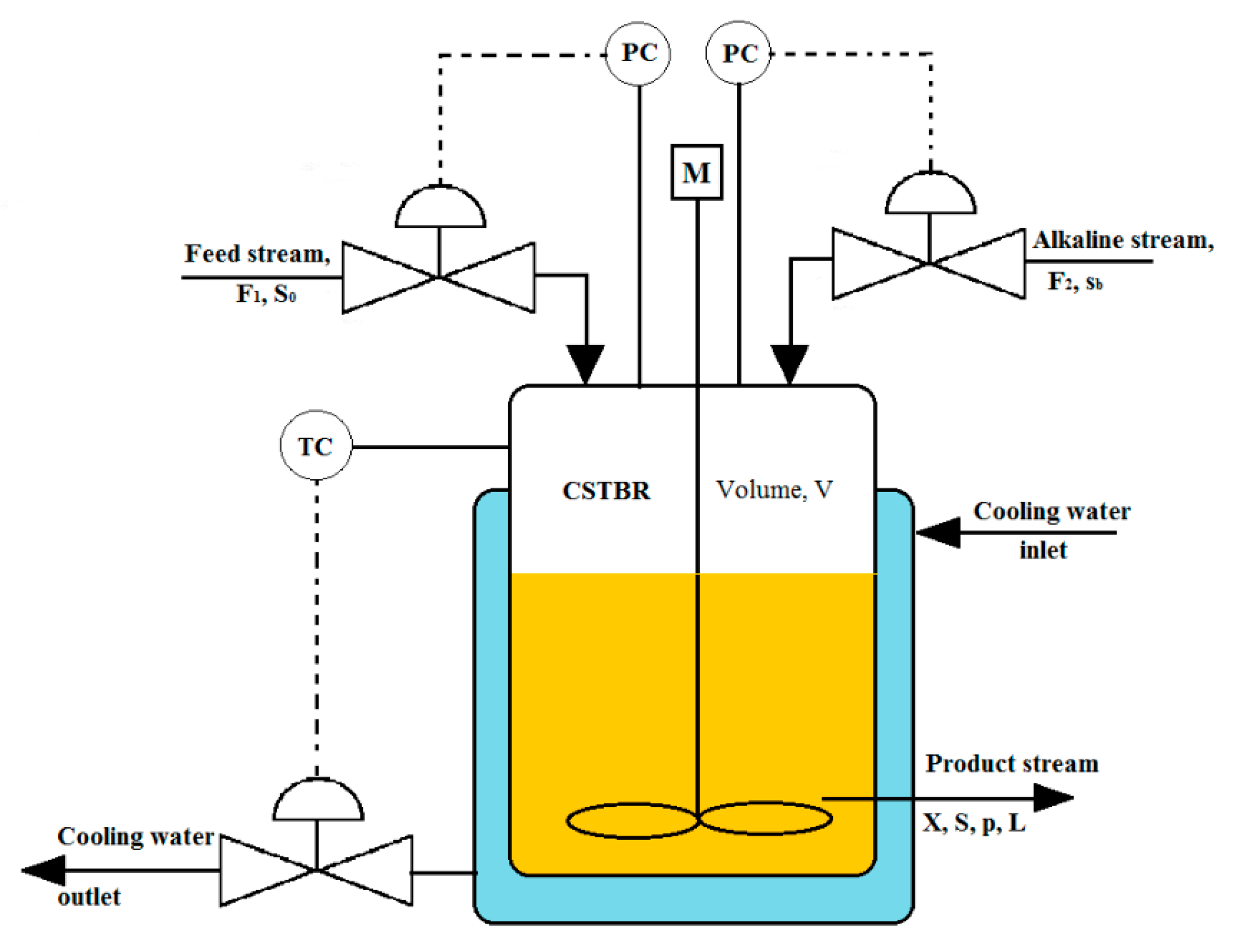
2.2.2. Mathematical Modeling of CSTBRs
- Ki the equilibrium dissociation constant for lactic acid
- sA molar concentration of sodium lactate (M)
- p molar concentrations of lactic acid (M)
- D = F1/V, dilution rate of the glucose feed stream (h−1)
- D1 = F2/V, dilution rate of the alkaline stream (h−1)
- YX/S yield coefficient for cell (g.g−1)
- t time (h)
2.2.3. Sensitivity Analysis
2.2.4. Calculation of Sensitivities
- Equations (22)–(25) and (28) are solved simultaneously with the help of initial conditions given in Equations (26) and (31) until the γ reaches its minimum value. The corresponding values of ρβ* and β* wre determined;
- (0) given by Equation (30) was calculated using the value of ρβ* with the help of the following equation:
- The objective sensitivity is then evaluated by solving the following equation:where,
3. Results
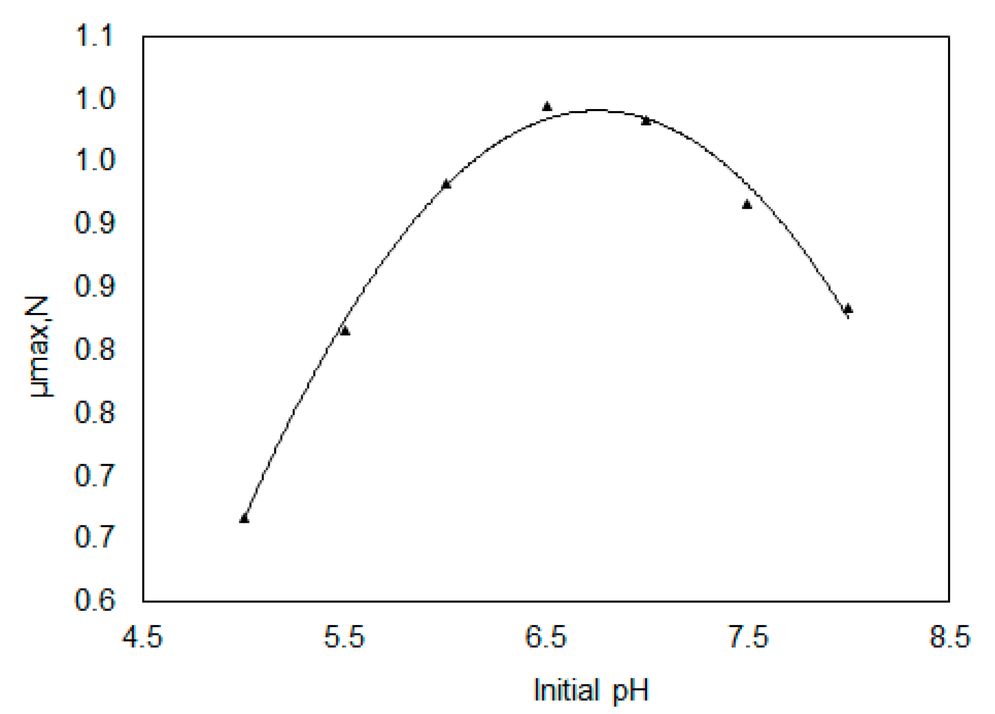
3.1. Determination of Kinetic Parameters of Lactobacillus Casei in Batch Culture
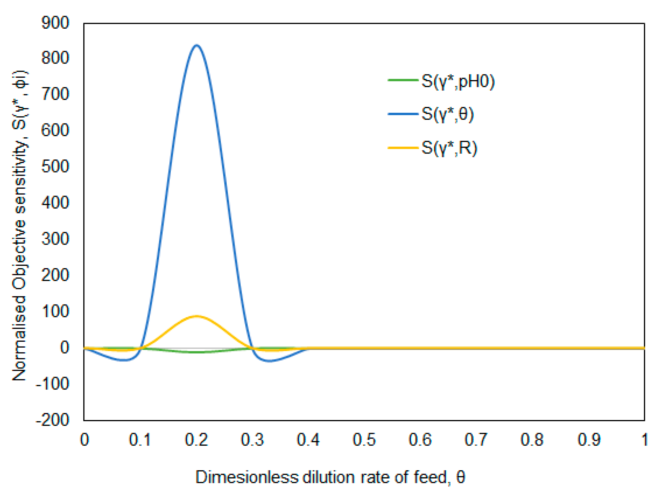
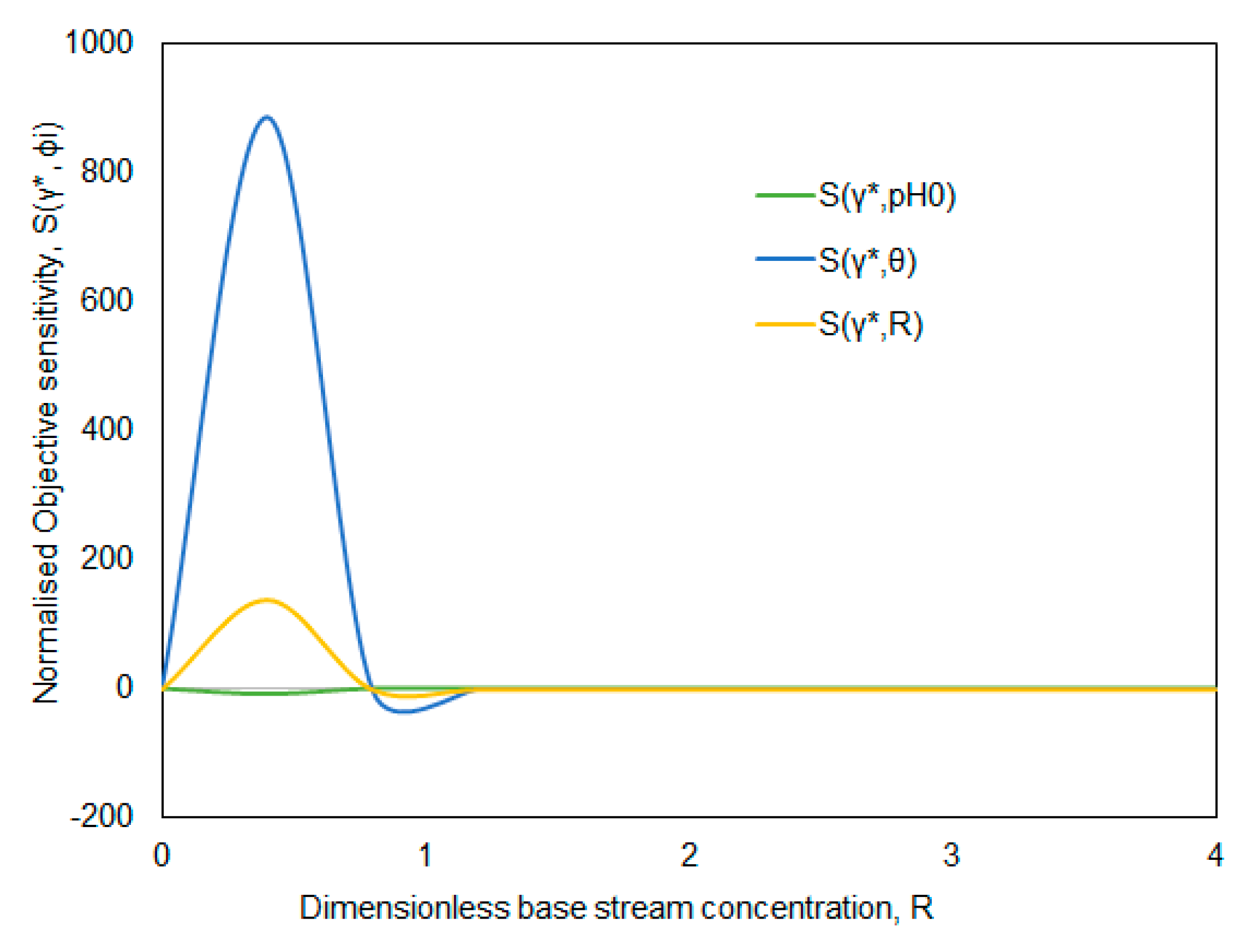
3.2. pH Sensitivity of a Continuous Stirred Tank Bioreactor
4. Discussions
5. Conclusions
Author Contributions
Funding
Acknowledgments
Conflicts of Interest
References
- Varma, A.; Morbidelli, M.; Wu, H. Parametric Sensitivity in Chemical Systems; Cambridge University Press: New York, NY, USA, 1999; ISBN 13-978-0-521-62171-7. [Google Scholar]
- Bilous, O.; Amundson, N.R. Chemical reactor stability and sensitivity: II. Effect of parameters on sensitivity of empty tubular reactors. AIChE J. 1956, 2, 117–126. [Google Scholar] [CrossRef]
- Morbidelli, M.; Varma, A. A generalized criterion for parametric sensitivity: Application to thermal explosion theory. Chem. Eng. Sci. 1988, 43, 91–102. [Google Scholar] [CrossRef]
- Chemburkar, R.; Morbidelli, M.; Varma, A. Parametric sensitivity of a CSTR. Chem. Eng. Sci. 1986, 41, 1647–1654. [Google Scholar] [CrossRef]
- Das, S.; Calay, R.K.; Chowdhury, R.; Nath, K.; Eregno, F.E. Product Inhibition of Biological Hydrogen Production in Batch Reactors. Energies 2020, 13, 1318. [Google Scholar] [CrossRef]
- Latif, M.A.; Mehta, C.M.; Batstone, D.J. Influence of low pH on continuous anaerobic digestion of iste activated sludge. Water Res. 2017, 113, 42–49. [Google Scholar] [CrossRef] [PubMed]
- Valle, B.; Aramburu, B.; Remiro, A.; Arandia, A.; Bilbao, J.; Gayubo, A.G. Optimal conditions of thermal treatment unit for the steam reforming of raw bio-oil in a continuous two-step reaction system. Chem. Eng. Trans. 2017, 58. [Google Scholar] [CrossRef]
- Waki, M.; Yasuda, T.; Fukumoto, Y.; Béline, F.; Magrí, A. Treatment of swine istewater in continuous activated sludge systems under different dissolved oxygen conditions: Reactor operation and evaluation using modelling. Bioresour. Technol. 2018, 250, 574–582. [Google Scholar] [CrossRef] [PubMed]
- Sayar, N.A.; Chen, B.H.; Lye, G.J.; Woodley, J.M. Modelling and simulation of a transketolase mediated reaction: Sensitivity analysis of kinetic parameters. Biochem. Eng. J. 2009, 47. [Google Scholar] [CrossRef]
- Sayar, N.A.; Chen, B.H.; Lye, G.J.; Woodley, J.M. Process modelling and simulation of a transketolase mediated reaction: Analysis of alternative modes of operation. Biochem. Eng. J. 2009, 47, 10–18. [Google Scholar] [CrossRef]
- Dutta, S.; Chowdhury, R.; Bhattacharya, P. Stability and response of bioreactor: An analysis with reference to microbial reduction of SO2. Chem. Eng. J. 2007, 133, 343–354. [Google Scholar] [CrossRef]
- Dutta, S.; Chowdhury, R.; Bhattacharya, P. Parametric sensitivity in bioreactor: An analysis with reference to phenol degradation system. Chem. Eng. Sci. 2001, 56, 5103–5110. [Google Scholar] [CrossRef]
- Morbidelli, M.; Varma, A. A generalized criterion for parametric sensitivity: Application to a pseudohomogeneous tubular reactor with consecutive or parallel reactions. Chem. Eng. Sci. 1989, 44, 1675–1696. [Google Scholar] [CrossRef]
- Das, S.; Banerjee, A.; Chowdhury, R.; Bhattacharya, P.; Calay, R.K. Parametric sensitivity of pH and steady state multiplicity in a continuous stirred tank bioreactor (CSTBR) using a lactic acid bacterium (LAB), Pediococcus acidilactici. J. Chem. Technol. Biotechnol. 2016, 91, 1431–1442. [Google Scholar] [CrossRef]
- Cats, A.; Kuipers, E.J.; Bosschaert, M.A.R.; Pot, R.G.J.; Vandenbroucke-Grauls, C.M.J.E.; Kusters, J.G. Effect of frequent consumption of a Lactobacillus casei-containing milk drink in Helicobacter pylori-colonized subjects. Aliment. Pharmacol. Ther. 2003, 17, 429–435. [Google Scholar] [CrossRef] [PubMed]
- De Vrese, M. Effects of probiotic bacteria on gastrointestinal symptoms, Helicobacter pylori activity and frequency and duration of antibiotics-induced diarrhoea. Gastroenterology 2003, 124, A560. [Google Scholar] [CrossRef]
- Miller, G.L. Use of Dinitrosalicylic Acid Reagent for Determination of Reducing Sugar. Anal. Chem. 1959, 31, 426–428. [Google Scholar] [CrossRef]
- Pandey, A.; Koruri, S.S.; Chowdhury, R.; Bhattacharya, P. Prebiotic influence of plantago ovata on free and microencapsulated l. Casei-growth kinetics, antimicrobial activity and microcapsules stability. Int. J. Pharm. Pharm. Sci. 2016, 8, 89–97. [Google Scholar]
- Lallai, A.; Mura, G.; Miliddi, R.; Mastinu, C. Effect of pH on growth of mixed cultures in batch reactor. Biotechnol. Bioeng. 1988, 31, 130–134. [Google Scholar] [CrossRef] [PubMed]
- Po, H.N.; Senozan, N.M. The Henderson-Hasselbalch equation: Its history and limitations. J. Chem. Educ. 2001, 78, 1499. [Google Scholar] [CrossRef]


| Microorganism | Lactobacillus casei (NCIM 5303) (Procured from the National Chemical Laboratory, Pune, India [18]) |
|---|---|
| Chemicals for DNS method (Merck Specialties Private Limited, India) | 3,5-dinitro salicylic acid, sodium hydroxide, sodium potassium tartrate |
| Equipment |
|
| Components | Amount (g) |
|---|---|
| Peptone | 1.0 |
| Beef extract | 0.8 |
| Yeast extract | 0.4 |
| Glucose | 2.0 |
| Sodium acetate trihydrate | 0.5 |
| Polysorbate 80 (also known as Tween 80) | 0.1 |
| Dipotassium hydrogen phosphate 0.2 | 0.2 |
| Triammonium citrate | 0.2 |
| Magnesium sulfate heptahydrate | 0.02 |
| Manganese sulfate tetrahydrate | 0.05 |
| Parameter | Definition | Parameter | Definition |
|---|---|---|---|
| α | U | ||
| β | θ | ||
| z | m | ||
| R | n | ||
| L | b | ||
| γ | c | ||
| τ | M1 | ||
| M2 |
| ϕi | σi |
|---|---|
| pH0 | |
| θ | |
| R |
| Kinetic Parameter | Value |
|---|---|
| µmax,opt (h−1) | 0.6 |
| KS (gL−1) | 0.08144 |
| YX/S (gg−1) | 0.238 |
| Yp/X (gg−1) | 3.36 |
| Yp/S (gg−1) | 0.8 |
| A | −3.8507 |
| B | 1.434 |
| C | −0.1062 |
| Sensitivity Coefficients S(γ*, ϕi) | Variable Parameters (Critical Values) | Sensitive Zone of Input Variables | Fixed Parameters | ||
|---|---|---|---|---|---|
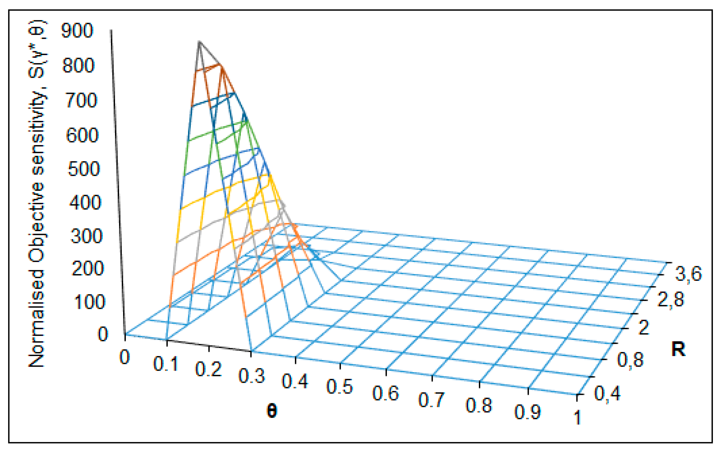
| S(γ*,θ) = 885 (Figure 6) | θC = 0.2 | RC = 0.4 | θ → 0.1–0.3 | R → 0–2.4 | pH0 = 6.75 |
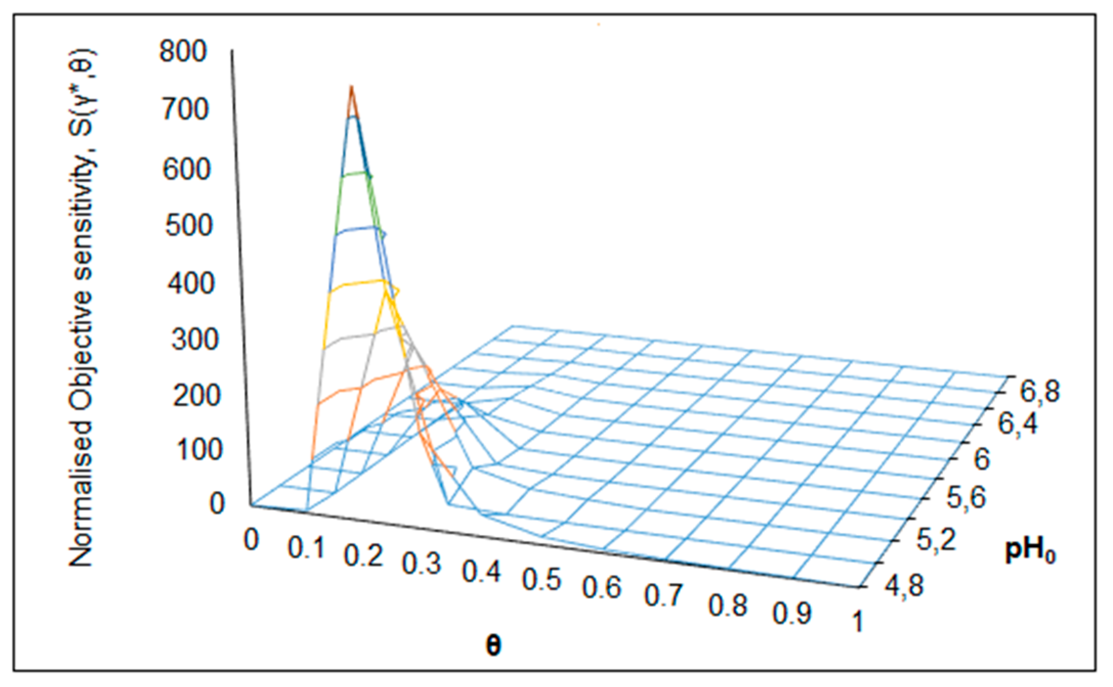
| S(γ*,θ) = 735 (Figure 7) | θC = 0.2 | pH0C = 4.8 | θ → 0.1–0.3 | pH0 → 4.8–6.0 | R = 0.2 |
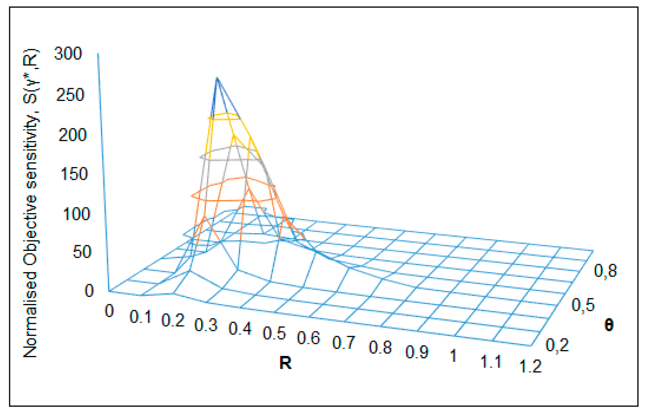
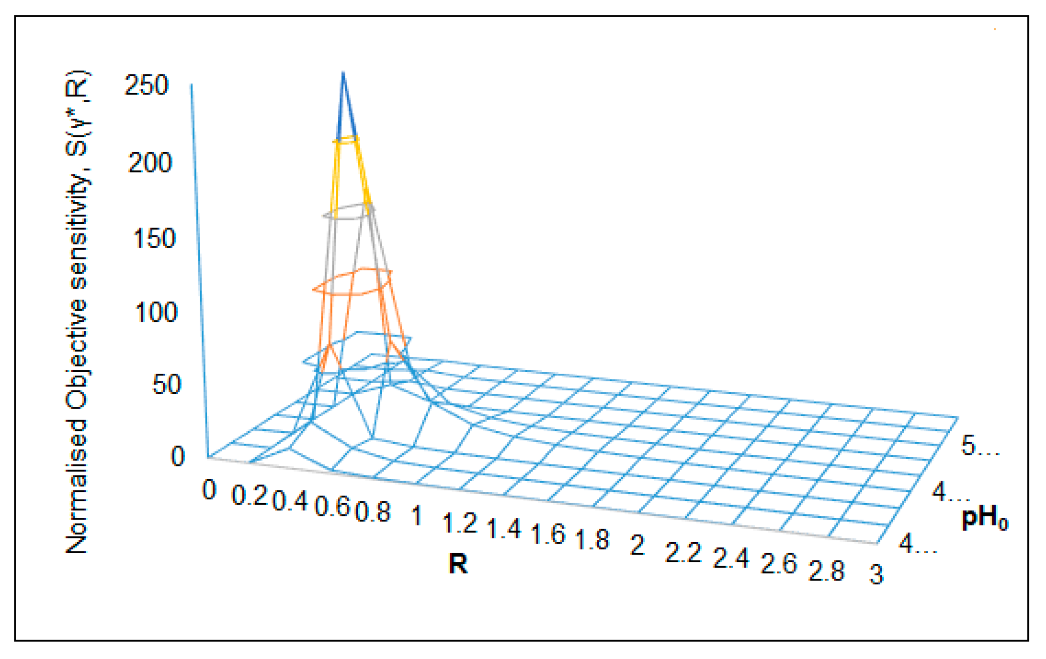
| S(γ*,R) = 285 (Figure 8) | RC = 0.2 | θC = 0.5 | R → 0.1–0.75 | θ → 0.05–0.7 | pH0 = 6.5 |
| S(γ*,R) = 245 (Figure 9) | RC = 0.4 | pH0C = 4.6 | R → 0.2–1.4 | pH0 → 4.2–4.6 | θ = 0.3 |
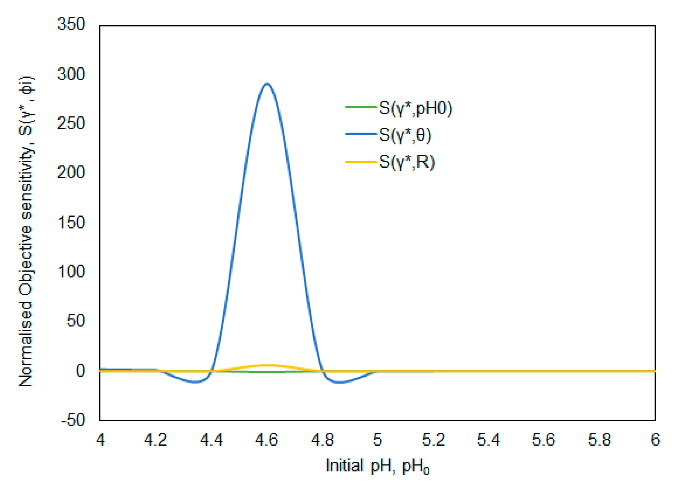
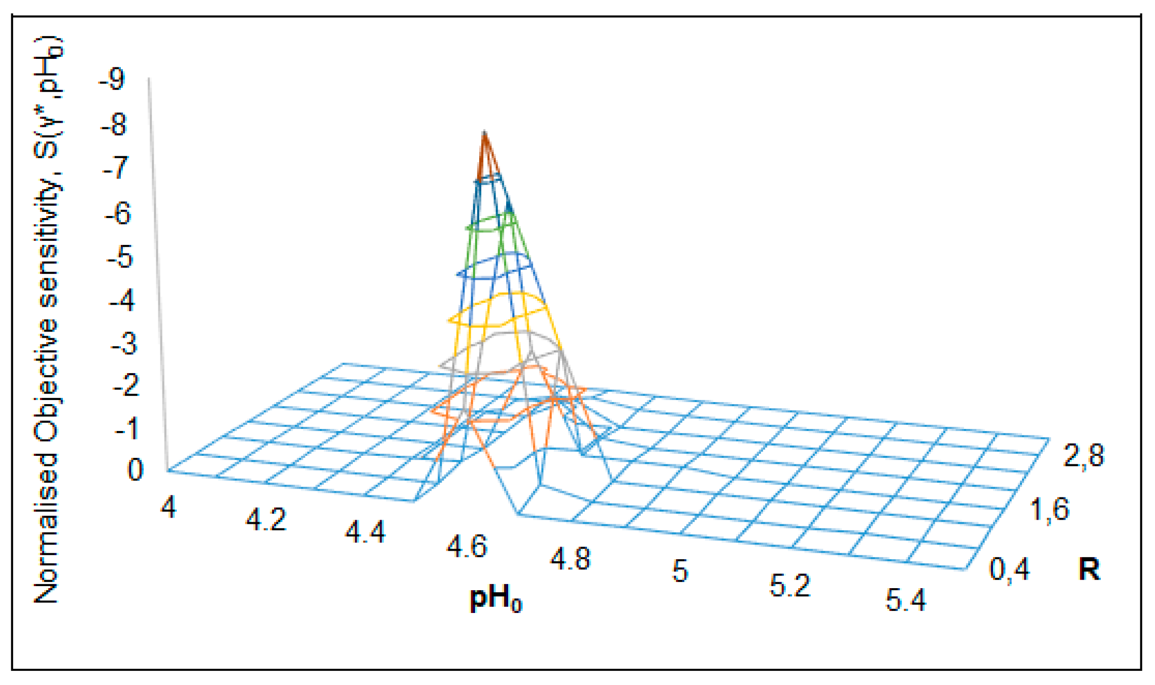
| S(γ*,pH0) = –7.8 (Figure 10) | pH0 = 4.6 | RC = 0.8 | pH0 → 4.5–4.8 | R → 0.4–2.0 | θ = 0.7 |
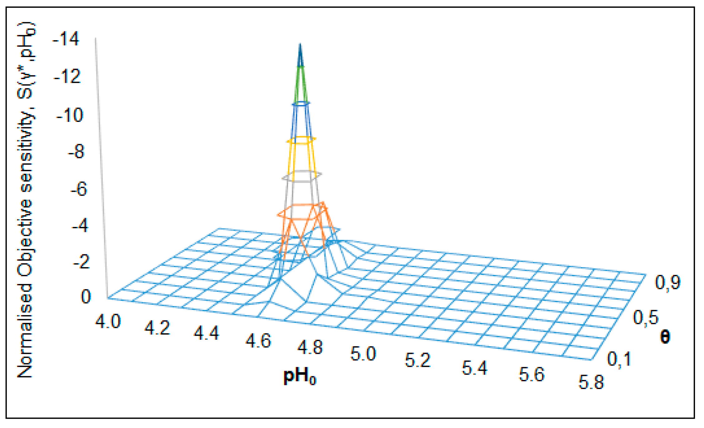
| S(γ*,pH0) = –13.8 (Figure 11) | pH0C = 4.6 | θC = 0.5 | pH0 → 4.45–4.85 | θ → 0.25–0.75 | R = 0.8 |
© 2020 by the authors. Licensee MDPI, Basel, Switzerland. This article is an open access article distributed under the terms and conditions of the Creative Commons Attribution (CC BY) license (http://creativecommons.org/licenses/by/4.0/).
Share and Cite
Das, S.; Calay, R.K.; Chowdhury, R. Parametric Sensitivity of CSTBRs for Lactobacillus casei: Normalized Sensitivity Analysis. ChemEngineering 2020, 4, 41. https://doi.org/10.3390/chemengineering4020041
Das S, Calay RK, Chowdhury R. Parametric Sensitivity of CSTBRs for Lactobacillus casei: Normalized Sensitivity Analysis. ChemEngineering. 2020; 4(2):41. https://doi.org/10.3390/chemengineering4020041
Chicago/Turabian StyleDas, Subhashis, Rajnish Kaur Calay, and Ranjana Chowdhury. 2020. "Parametric Sensitivity of CSTBRs for Lactobacillus casei: Normalized Sensitivity Analysis" ChemEngineering 4, no. 2: 41. https://doi.org/10.3390/chemengineering4020041
APA StyleDas, S., Calay, R. K., & Chowdhury, R. (2020). Parametric Sensitivity of CSTBRs for Lactobacillus casei: Normalized Sensitivity Analysis. ChemEngineering, 4(2), 41. https://doi.org/10.3390/chemengineering4020041