1. Introduction
Process engineering involves mechanistic models on different scales, ranging from pure-substance over mixture properties up to models for different apparatuses and flowsheets. On each scale, the corresponding model involves model parameters. Generally, these model parameters are not known a priori, but must be determined such that the model predictions match measurements from experiments. This procedure is designated as parameter estimation by model regression in the following. This work describes recent progress that has been made in implementing least-squares regression approaches in an industrially relevant context, including efficient error propagation from one scale (e.g., thermodynamic mixture properties) to another (e.g., flowsheets described by the MESH equations).
Least-squares regression probably belongs to the most popular methods of parameter estimation. The reason is that one can show that this method leads to the best parameter estimates assuming that the ground truth is known and the experimental measurements are normally and independently distributed around this ground truth (for more details, cf. the textbook [
1]). However, these two assumptions are never strictly fulfilled in practice: Neither the ground truth is known nor are the measurements normally distributed. Thus, from a practical point of view, least squares can rather be considered as one possibility to measure the distance between model prediction and experiment. Other measures for the distance adapted to special situations, such as strong deviations of the measured data from normal distribution due to outliers, are known as well [
2]. More recently, Bayesian parameter estimation has gained some attention [
3,
4]. Here, however, we restrict ourselves to the least-squares approach, which in countless situations has led to satisfactory parameter estimates (for a recent review, cf. [
5]).
In the context of chemical engineering, three challenges are encountered when it comes to regression: The first is that measurement errors are present not only in the measured quantities corresponding to model predictions but also in those corresponding to the model inputs. The second challenge results from multiple model outputs and their respective weights in the loss function of the regression: Ideally, weights are obtained from the variances of the measurement errors [
6], which are not known exactly. They can be estimated as well, resulting in tedious iterative loops [
3,
6]. For the practitioner, however, weights have only a limited physical meaning; the more important question is how well can the model describe a set of data with different output quantities. Finally, the third challenge consists in propagating the error estimates of the model parameters through different model scales, since these are usually implemented in different environments with limited interfaces. Thus, methods are needed that encode the parameter estimates and their errors obtained from the performed regression, e.g., for mixture properties from experiments in the lab, such that these can be easily used by flowsheet simulators, which describe the properties of entire processes. All three challenges are addressed in the present contribution.
In
Section 2, we compare different methods to numerically solve parameter estimation problems for highly nonlinear thermodynamic models for pure-substance and mixture properties. These could be, for example, gE-models [
7,
8] or equation-of-state approaches such as PC-SAFT [
9,
10]. Further references can be found in the textbook [
11]. In conventional least-squares regression, it is assumed that measurement errors occur only in the model outputs. Measurement errors in both model inputs and outputs are accounted for by data reconciliation or errors-in-variables methods [
12,
13]. Data reconciliation aims to correct the measurement errors by the incorporation of models for the process. Models at different scales can be employed, ranging from simple models describing only parts of the process, e.g., the conservation of mass, to complex models, which are designed to describe the process completely. Data reconciliation does not differentiate between input and output quantities. Therefore, data reconciliation combined with parameter estimation can serve as an errors-in-variables model for parameter estimation. Errors-in-variables methods lead to restricted nonlinear optimization problems, where the number of equality constraints increases with the number of measured points. This can become a challenging optimization problem, requiring advanced solvers which are capable of dealing with sparsity. In industrial environments, such solvers are not always available. We therefore show how the constrained least-squares optimization problem can be recast as an unrestricted problem. This idea originates in the work by Patino–Leal [
14,
15]. Our contribution consists in an alternative derivation of this formulation and in a comparison of the regression results from conventional least squares, error-in-variables least squares with constraints, and the reformulation without constraints.
Section 3 provides the comparison of the different parameter estimation strategies for two specific thermodynamic examples.
The second challenge, related to a suitable choice of weights in a multivariate regression problem with unknown variances of the measurements, is tackled in a multi-criteria framework in
Section 4. An adaptive scalarization scheme is used to choose the weights such that, in the case of conflicting regression objectives, the resulting Pareto boundary is computed with the least numerical effort [
16,
17,
18]. This approach has been successfully applied to parameter estimation in the context of molecular simulations [
19] and the parametrization of equations of state [
20]. In this work, the multi-criteria framework will be, to the best of the authors’ knowledge for the first time, extended to the determination of process parameters of a flowsheet simulation.
Finally, in
Section 5, we discuss the third challenge dealing with error propagation. It is well known that an estimate of the covariance matrix for the model parameters can be obtained from an analysis of the regression results [
21,
22]. In the present paper, we review different measures for the errors resulting from this matrix. Furthermore, we propose a scheme allowing for efficient error propagation in the case where the regression task has been performed in a model environment different from the one eventually employing the parameter estimates. This situation frequently occurs in process engineering, since the properties of pure substances and their mixtures are estimated from regression of thermodynamic models to lab experiments and are then used by flowsheet simulators.
We would like to mention that all of the described algorithms were implemented in in-house tools of the industrial partners with very specific interfaces. Therefore, employing existing commercial solutions was not an option.
2. Parameter Estimation Approaches
The physical process involved in measuring an input–output relation can be described by the regression model
Here, the measured value of the output is obtained by evaluating the model at the input and adding an error , which is assumed to be normally distributed with zero mean and standard deviation . The model depends on the vector of parameters , which are to be estimated from a set of measured data .
At this point, the input quantities may be considered as vectors of dimension and , f, as vectors of dimension . If , we assume that the measurement errors are uncorrelated, i.e., is a diagonal -matrix. This assumption is sufficient for many situations in practice, because the measurements are performed by independent sensors not being correlated with each other. Since, in most cases, estimates for the correlations of measurement errors are not available, we discard them for the sake of a simpler notation.
If the model is a linear function of the parameters to be estimated, a linear parameter-estimation problem has to be solved. This leads to a quadratic optimization problem and can, in principle, be solved analytically. On the other hand, if the model depends nonlinearly on the parameters, the parameter-estimation problem becomes nonlinear as well. In this case, a nonlinear optimization method is required. In thermodynamics, many highly-nonlinear effects occur and, therefore, this work focuses on nonlinear parameter estimation problems. The methods used can also be applied to linear problems.
2.1. Least Squares
The simplest and most common strategy for the estimation of model parameters from measured data is the method of least squares. The approach consists in minimizing the sum of squared residuals, which are defined as the differences between the measured values
and the ones predicted by the model for the corresponding measured inputs
. It can be derived from the maximum-likelihood estimator under the condition that all measurement errors are normally distributed and independent. The detailed derivation can be found in numerous textbooks (e.g., [
23]). Therefore, only a short summary is given here. The best values for the model parameters
are calculated by maximization of the probability to obtain the measured dataset
, leading to the optimization problem
For the multiple output case, the single terms of
should formally be written as
, whereas, for diagonal matrices, Equation (
3) can be interpreted component-wise. In the following, we employ the simpler notation. In Equation (
1), the measurement error is assumed to appear only in the model outputs, the errors of the input quantities
are not considered. In thermodynamic applications (and many others), the differentiation between input and output quantities is often only based on the formulation of the model. However, both quantities are subject to measurement errors.
2.2. Reconciliation Formulation with Constraints
To include errors of input variables, a simultaneous data reconciliation and parameter estimation problem is proposed [
12,
13], which is also known as the errors-in-variables model [
14].
where
denotes the errors of the input variables. However, the price for including the errors of the input variables is high: Optimization solvers specialized for least-squares functions usually require derivatives for every residual separately. Here, the introduction of
additional optimization variables increases the size of the gradient from
to
and the number of residuals from
to
. The size of the Hessian matrix increases by the square of the factors. Most of the additional entries are zeros, and it is possible to calculate the matrices efficiently. However, storing them in memory efficiently is more difficult and requires to use solvers with implementations, which are adapted to these structures.
As shown in
Section 2.3, the problem can be reformulated and approximated to a form without these additional variables but still including the errors of the input variables (see Equation (
15)). Before addressing this, we reformulate Equation (
5) using constraints, which leads to a constrained optimization problem
This version can directly be applied to implicit models and represents the first step in reducing the number of optimization variables.
2.3. Reconciliation Formulation without Constraints
In Equation (
6), the input and output variables are treated on equal footing, which is expressed by collecting them in a single vector
, and the corresponding errors
into one diagonal matrix. Furthermore, the quantity
g is introduced as
This form has the additional benefit that it can be directly applied to models given only implicitly (i.e.,
). Equations (
6) and (7) with the substitution Equation (
8) constitute a restricted least-squares optimization problem, where the number of constraints scales with the number of measurements
N. For large
N, advanced optimization solvers are necessary to solve this problem. In this section, a method is presented that leads to an unrestricted optimization problem, which is equivalent to Equations (
6)–(
8). This method is due to Patino–Leal [
14,
15]. In the original work, it was derived in a Bayesian framework. Here, we present an alternative derivation based solely on the restricted problem (Equations (
6)–(
8)). This reformulation relies on a linearization of the constraints in Equations (7) and (
8), and is sketched below. To remove the additional optimization variables from Equation (
6), the constraints (i.e., the actual model equations) are linearized with respect to the variables
around some point
:
Note that, for linear models, the approximation is exact, and, for explicit models, the
dependence is already linear by definition of
g. The impact of this approximation on the results strongly depends on the accuracy of the approximation in the vicinity of the actual result, which in turn relies on the choice of the point, which is used for the linearization. Now, while the number of optimization variables has not been reduced yet, the minimization problem with respect to the
variables, for fixed parameter values
, has a much simpler structure-quadratic objective function and linear constraints—and can be solved analytically. It is very similar to the problems appearing in data reconciliation dealing with unmeasured variables described, e.g., in [
12]. The analytical solution is given by
with the abbreviations
Inserting these results in the optimization problem in Equation (
9) yields
This strategy can readily be applied to models with multiple inputs and outputs and even works directly for implicit models. The values
are called linearization points and play a similar role as the additional variables
in the reconciliation strategy given in Equation (
5). However, in contrast to Equation (
5), the
are calculated within the evaluation of the residuals. For large problems, this is an advantage compared to Equation (
5), where, due to the introduction of a high number of extra optimization variables, the optimization takes substantially longer. On the other hand, in Equation (
15), the additional calculations are performed within the evaluation of the objective, and thus the numerical effort grows only linearly with the number of data points.
Thus far, the reformulation leading to Equation (
15) is based on an initial linearization of the constraints. The optimal point for linearization of the constraints is the true value of the measured quantities, because there the nonlinearity of the model does not play a role any longer. For reliable measurements, the measured values are a reasonable approximation for the linearization points
. For different linearization points, the linearization has to be adapted in a fixed-point iteration after each solution of the unrestricted problem Equation (
15) in the following way [
14,
15]:
which is expected to converge reliably also in the presence of non-linearities.
2.3.1. Computational Aspects
Optimization algorithms specialized to least-squares problems [
24] have been developed which offer a significant gain in performance compared to conventional solvers which do not take advantage of the least-squares structure. The performance is enhanced by deriving an approximation of the Hessian matrix from the gradients of the individual terms instead of from the gradient of the sum of squares. The Hessian of a quadratic expression contains the first and the second derivatives of the argument. Since the gradients of the individuals terms are, in most cases, already calculated to determine the gradients of
, this part of the Hessian can be evaluated exactly without additional costs and only the part involving second derivatives has to be approximated. Different methods to incorporate this information exist: Spedicato and Vespucci [
24] proposed specialized Hessian update strategies, whereas Schittkowski [
25] reformulated the individual objective terms as constraints and approximates the Hessian of the constraints individually.
Those specialized solvers usually rely on a sum of squares form of the objective function. The strategy given by Equation (
15) does not have this structure. It is, however, possible to reformulate the objective function
into a form consistent with standard least-squares algorithms. To this end, the
decomposition of the matrix
, with
defined by
, is introduced. Then, the inverse matrix in Equation (
15) can be obtained and the objective function can be equivalently written as
where the vectors
are calculated by solving the linear system of equations
The computational costs are only slightly increased, since Equation (
15) requires a matrix inversion as well. A detailed derivation is contained in
Appendix A.
2.3.2. Linearization Points
A simple version of Equation (
15) is to use the measured values
as an approximation of
. However, if one wants to use the optimal values for the linearization points
given in Equation (
16), an additional loop inside the residual evaluation is required, which leads to significantly more model evaluations. One solution to this problem is to only use
as starting value in the first iteration of the optimization (or whenever a misfit is detected) and the final value of the previous iteration otherwise. Then, Equation (
16) may require only a small numbers of iterations, in the extreme case just one. For strongly nonlinear models and parameter values far from optimal (or even physically reasonable) ranges, however, the convergence may be limited. In such cases, it is preferable to start the optimization with the approximate formulation, until reasonable parameter values are obtained.
An alternative formulation for the iteration in Equation (
16) is
with
(as in the previous section). This requires an algorithm for the linear least-squares problem with equality constraints given in Equations (
20)–(22). QR decomposition is a typical component of such algorithms, but it is no longer necessary to use it explicitly. The objective function
of Equation (
17) can be calculated directly as
. The derivation is provided in
Appendix B.
3. Comparison of Parameter Estimation Strategies
To demonstrate the behavior of the different regression strategies presented in
Section 2, two examples from thermodynamic practice are discussed.
3.1. Example: Vapor Pressure
The standard DIPPR model for the vapor pressure of methanol was chosen as a first test model to compare the different regression strategies. The measured dataset was provided by BASF SE and consists of 40 data points for the (logarithmic) vapor pressure and the temperature. The model describes the temperature dependence of the logarithmic vapor pressure according to
Herein, a, b, and c denote the model parameters to be estimated, and pressure p and temperature T are given in units of Pa and K, respectively. The model parameters were determined using four different regression strategies with three different initial parameter values:
the ordinary least-squares strategy
(Equation (
3))
the reconciliation strategy
(Equation (
5))
the approximate error-in-variables model
(Equation (
17)) without linearization point optimization
the full error-in-variables model
together with Equation (
20) (
)
The results are shown in
Table 1. They include the observed run time of each regression run. These values were obtained by taking the mean value of repeated micro-benchmark runs on a Windows machine with an Intel Core i7-7700 CPU and 2 × 8 GB DDR4-2400 main memory. The parameter values agree with each other within a few percent, except for the strategies
and
for the third initial value. The error was defined as the minimum value of the objective function
and therefore expected to differ between the methods. Note that the highest error was obtained by
, because all other methods split the error between input and output. The reconciliation strategy
required many iterations. However, the approximate version
yielded, except in one case, almost the same result with much fewer iterations. The last strategy
agreed with the third one, but took the highest time in total, because of the additional loop for the linearization points. For the third initial value, the last two strategies converged to a different local minimum; however, the effect of the varying parameter sets on the model prediction was very small. The model predictions for the corresponding cases are shown in
Figure 1. The difference between any two predictions evaluated at the data points was smaller than 0.04 (i.e., below 0.5% of the absolute value). If only the different strategies starting from the same initial point were compared, this bound reduced to 0.0003. The fact that different parameter sets led to similar model predictions was related to the correlations between the model parameters. The variation of one parameter was compensated by adjusting a correlated parameter, and the parameters could not be independently estimated from the data. For this example, the ordinary least-squares strategy (
) already worked quite well, and we compared it with respect to the results and the performance of the other methods. The strategy
works well for sufficiently small problems, whereas the error-in-variables strategy
is also suited for larger problems. The last strategy
is useful for situations where the approximation in
does not work well and the problem size is too large for
.
3.2. Example: NRTL
For a second comparison of the different regression problem formulations, the NRTL model for a water–methanol binary mixture was chosen. For this test, the simplest parameterization of the NRTL model was used
which has three parameters (
). Here,
denotes the excess Gibbs free energy, which is normalized by temperature
T and gas constant
R. The model has a single input
, which is the mole fraction of methanol in the liquid phase, and
being the corresponding mole fraction of water is not independent. The dataset, which already has been published in [
17], contains the temperatures and the molar fractions of methanol in the liquid and the vapor phase. Based on the extended Raoult’s law, from these data activity coefficients
for both phases can be estimated. The regression was performed using the differences between the logarithmic activity coefficients
estimated from the experimental data and the model. Since the data contained no information about the measurement errors, a standard deviation of
4% was assumed for the activity coefficients. For the mole fractions, the standard deviation was set to 4% for values above 0.1. Below this threshold, a constant standard deviation of 0.004 was used. The parameter
was not optimized, but set to a fixed value of
, since it could not be reliably estimated from this dataset.
The results are summarized in
Table 2, which contains the parameter values, the numbers of needed iterations, and timing estimates obtained with the same settings as in
Section 3.1. For all regression calculations, the NLPLSQ solver [
25] was used with a residual guess of 10 and accuracy settings of
and
(QP).
Figure 2 shows the data together with the corresponding model predictions for all four strategies. The model curves are very similar. The maximum of the absolute differences between the model predictions evaluated at the data points was 0.013 (i.e., about 1% of the value of
close to
) and reduced to 0.003, if strategy
was excluded.
As in the previous example, the results of all four strategies agree well with each other. While the strategies , , and use different objectives for the optimization to include the errors of input variables, the results of these three strategies can be considered identical, and even was only slightly different. The effect of the input-variable errors, for which homogeneous estimate of was assumed, seemed to be small in this example. In addition, the approximation used in was already sufficient, such that did not yield an improvement. The time for all four strategies was much larger than in the first example, because the dataset consists of 540 points. This was still feasible for method , but the difference in speed compared to and was much more significant here. Therefore, the methods and are better suited to handle cases appearing in practice that contain large datasets. Despite the large dataset, the current model was rather small, since it used only one input variable, two output variables, and two parameters. The size of the optimization problem in increased with the number of input and output variables, so that much larger problems could easily occur.
In summary, all strategies to take input-variable errors into consideration agree well with each other, and differ only slightly from the ordinary least-squares strategy. However, in general, when the input errors are significant, deviations are expected. In cases where the ordinary least-squares strategy does not yield satisfactory results or it is expected that significant input variable errors are present in the data, the two other strategies are available as alternatives. The reconciliation strategy is simpler than and , but its numerical effort grows for large-size problems.
4. Multi-Criteria Parameter Estimation
The regression approaches considered thus far, in
Section 2 and
Section 3, strongly depend on the standard deviations of the data. However, in practice, often the standard deviations of the measured data are not well known or the measuring sensors might not be reliable. Thus, it is essential to know in how far the estimated parameters depend on changes in the estimates of the variances. A solution to this problem is provided by performing parameter estimation in a multi-criteria framework. Here, one can define multiple sums of least squares as objectives to be minimized. In general, if the system is over-defined, not all objectives can be minimized simultaneously and the result is a set of Pareto optimal solutions, lying on the so-called Pareto front [
26].
Exploration of the Pareto front corresponds to a sensitivity analysis of the weights of the different sums of squares. Thus, using a separate objective function for each data point, one performs a sensitivity analysis of the standard deviations. If the number of data points is large, in practice, it is more advantageous to group data points to only a few least-squares functions, e.g., according to their physical unit, order of magnitude, or the reliability of their error estimates. This kind of grouping has been proven useful in [
19,
20].
Furthermore, the Pareto front indicates how close the model can at all get to the data. As demonstrated via an example in
Section 4.2, this reveals valuable information about systematic deviations of single measurement values from the model predictions, thus providing hints for possible gross errors. Finally, as clarified in the Introduction, a statistically rigorous estimate of the variances would, for a multivariate regression, involve solving an iterative loop between minimizing the residual sum of squares and estimating the variances. Performing this iteration is completely avoided by calculating the Pareto front, which contains all possible outcomes of the regression.
In this section, we focus on data from industrial process plants. However, the general method can be applied to arbitrary parameter estimation problems. For instance, it could be used for the examples from thermodynamics in
Section 3 as well.
4.1. General Framework
In the following, we describe a general framework for multi-criteria parameter estimation using process data. Model parameters can be fitted both to measured data from one and multiple datasets (or experiments). In the context of industrial process data, multiple datasets correspond, e.g., to multiple operating points. In general, two types of model parameters appear:
which are independent of the operating point and
,
which depend on the operating point, where
is the number of operating points. Establishing the connection to
Section 2, the parameters
are associated with the inputs
in Equation (
1). A single objective
,
to be minimized takes the form
where
denotes the number of measured quantities (or tags) and
the measured value of tag
j at operating point
p assigned to objective
i, e.g., according to the physical unit with index
i. The corresponding standard deviation is denoted by
whereas
is the model prediction for quantity
j attributed to objective
i. We can define several of these objectives summarized as
, and the multi-criteria optimization problem to be solved reads
Pareto optimal solutions of this problem can be obtained using scalarization algorithms [
27,
28,
29], which combine the objectives to a single scalar function, which is then passed to an optimization solver. In the following, we employ an adaptive method provided by the sandwiching algorithm [
16,
30,
31].
4.2. Example: Distillation Column
We present the application of multi-criteria parameter estimation to a real-world industrial process. This example depicts a distillation column which is part of a downstream separation process, operated by LONZA AG at one of their production sites. The flowsheet is displayed in
Figure 3.
The column feed is a mixture of 15 known and some unknown components and the main product is obtained at the top drain. The process model is implemented as a steady-state simulation in the flowsheet simulator CHEMCAD. Here, the column consists of 53 stages. Available real process data are the total flow rates of the three streams 1, 2, and 3 and the temperature measurements at stages 1, 2, 19, 38, 46, 52, and 53. We adjusted the model to these data at a single operating point. The composition of the feed was measured as well and, in the simulation, was fixed to these data. It was not practical to define a separate objective for each measured quantity, since the interpretation of the results would become too involved. Therefore, we defined (only) two objectives to be minimized, one least-squares function for the flow rates and one for the temperatures:
Since reliable estimates for the standard deviations are not available, we set them to the default values
and
. The so-defined objectives can then be interpreted as the average deviations between simulated and measured values given in units of standard deviations. The model parameters to be adjusted are the total feed flow rate, the reflux ratio, the reboiler specification (given by the mass fraction of the main product in the bottom drain), and a global value for the tray efficiencies of all stages. Those optimization variables are summarized in
Table 3.
The multi-criteria optimization problem was solved using the sandwiching algorithm [
16,
30,
31] together with the NLPQLP solver [
32]. We obtained four Pareto points and the interpolated Pareto front is shown in
Figure 4.
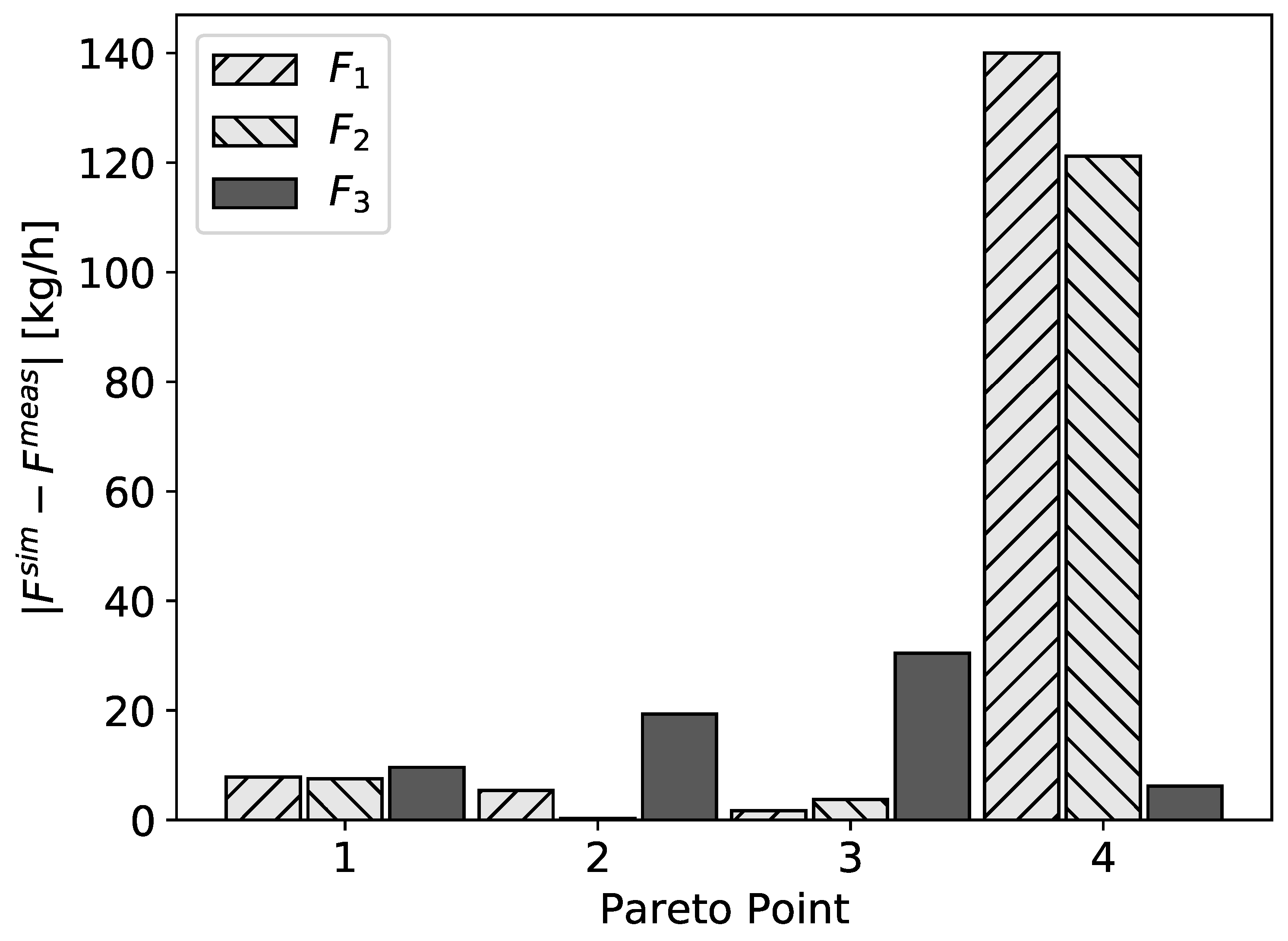
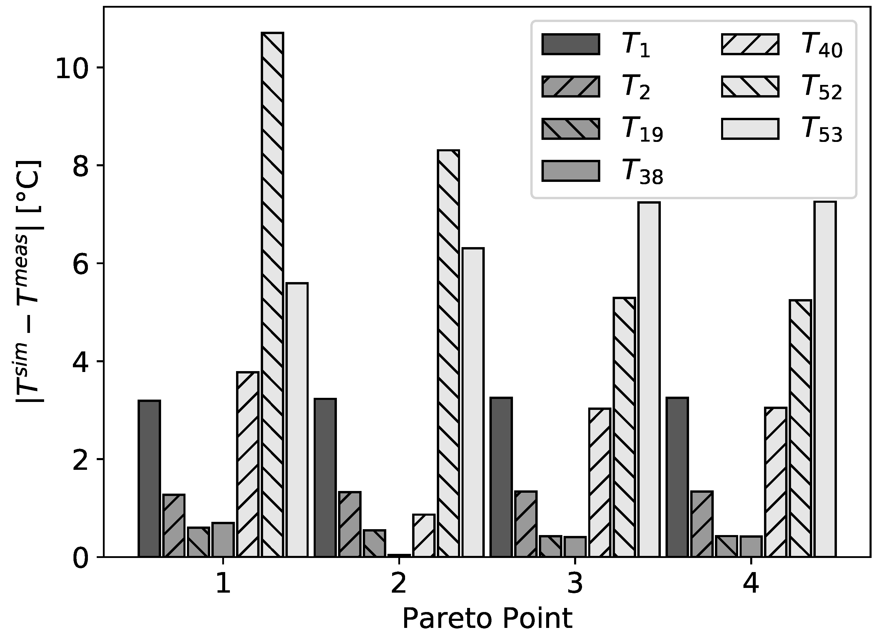
One can clearly see that it is not possible to minimize both objectives simultaneously. Navigation on the Pareto front shows the dependence of the resulting parameters on variations of the variances and allows then to choose a set of model parameters which fit either the flow rates or the temperatures better. This decision is beyond the scope of this work, since it has to be made relying on context knowledge and is therefore up to the engineer who knows which measured data are more reliable and should be described better. To study the contributions of the different measured points to the objectives, the residuals at the Pareto points are displayed in
Figure 5 and
Figure 6.
For all four Pareto points, the residuals of the temperatures showed systematic deviations for and at the bottom of the column. They were in agreement with the observation that the corresponding temperature sensors at the real column did not work well and might have provided erroneous results. Thus, our framework is well suited for the detection of such systematic deviations.
5. Error Estimates
Having discussed how model parameters can be estimated from data, we now present strategies to quantify the errors of the obtained parameter values and corresponding model predictions [
23]. Well-known error estimates are the parameter confidence regions, the parameter confidence intervals, and the prediction bands. They are derived from a quadratic approximation of the least-squares function
around the optimal parameter values
. At this point, the linear contribution to the approximation vanishes. From the quadratic contribution, the parameter covariance matrix
C is obtained, which is a local measure of the change in the model under variations of the parameters. The parameter covariance matrix is the inverse of the Fisher information matrix (FIM), i.e.,
, which is calculated by
where
N and
are the number of data points and model parameters, respectively. Here,
s can be any of
defined in Equations (
3) and (
5), or Equation (
17), and the
are the individual terms such that
. A more general form of the FIM for multiple outputs and differently structured data points is given in
Section 5.2. Before that, a short review of error estimates is given.
5.1. Confidence-Region Estimates
The parameter confidence region is a set in parameter space which contains the true parameter values with a certain probability, the so-called confidence level
, e.g., 95%. It can be obtained by statistical theory under the assumption that the data used for the regression are obtained from the model with the true parameter values and an error which is independent and normally distributed (see
Section 2). The parameter confidence region is then given by [
23]
where
is the corresponding quantile of the FisherF distribution. This inequality describes an ellipsoid centered at
, with main axes along the eigenvectors of
C and proportional to the square root of the corresponding eigenvalue. The orientation of the ellipsoid in space depends on the off-diagonal elements of
C.
The confidence intervals [
23] provide the same information as the confidence region but for the individual parameters. They are the projections of this ellipsoid onto the coordinate axes, multiplied by the quantile of the StudentT distribution
instead of the FischerF distribution
The confidence region and confidence intervals are illustrated in
Figure 7 for a two dimensional example.
In the next step, based on the parameter errors, we can determine the error of the model evaluation. The estimate for the error of the model prediction obtained from the confidence region is the prediction band [
23] (also called confidence band). It provides error estimates for the evaluation of the model at arbitrary points
It is also possible to calculate error estimates based on the confidence intervals of the individual parameters. If the covariance matrix
C is (close to) diagonal, i.e., the parameters are uncorrelated, Equation (
35) simplifies to
On the other hand, if the covariance matrix cannot be assumed to be diagonal, an upper bound for the error is given by
because the off-diagonal elements of the covariance matrix are always bounded by
. Equations (
36) and (
37) are the typical formulas for error propagation. These estimates, however, are very conservative in the case of large parameter correlations. The confidence intervals are practically the projections of the confidence region onto the coordinate axes, since the quantiles in Equations (
33) and (
34) differ only slightly numerically. Therefore, this approach corresponds to the approximation of an ellipsoid by its bounding box (aligned to the coordinate system). For large parameter correlations, the confidence region becomes more elongated and tilted away from the coordinate axes. In
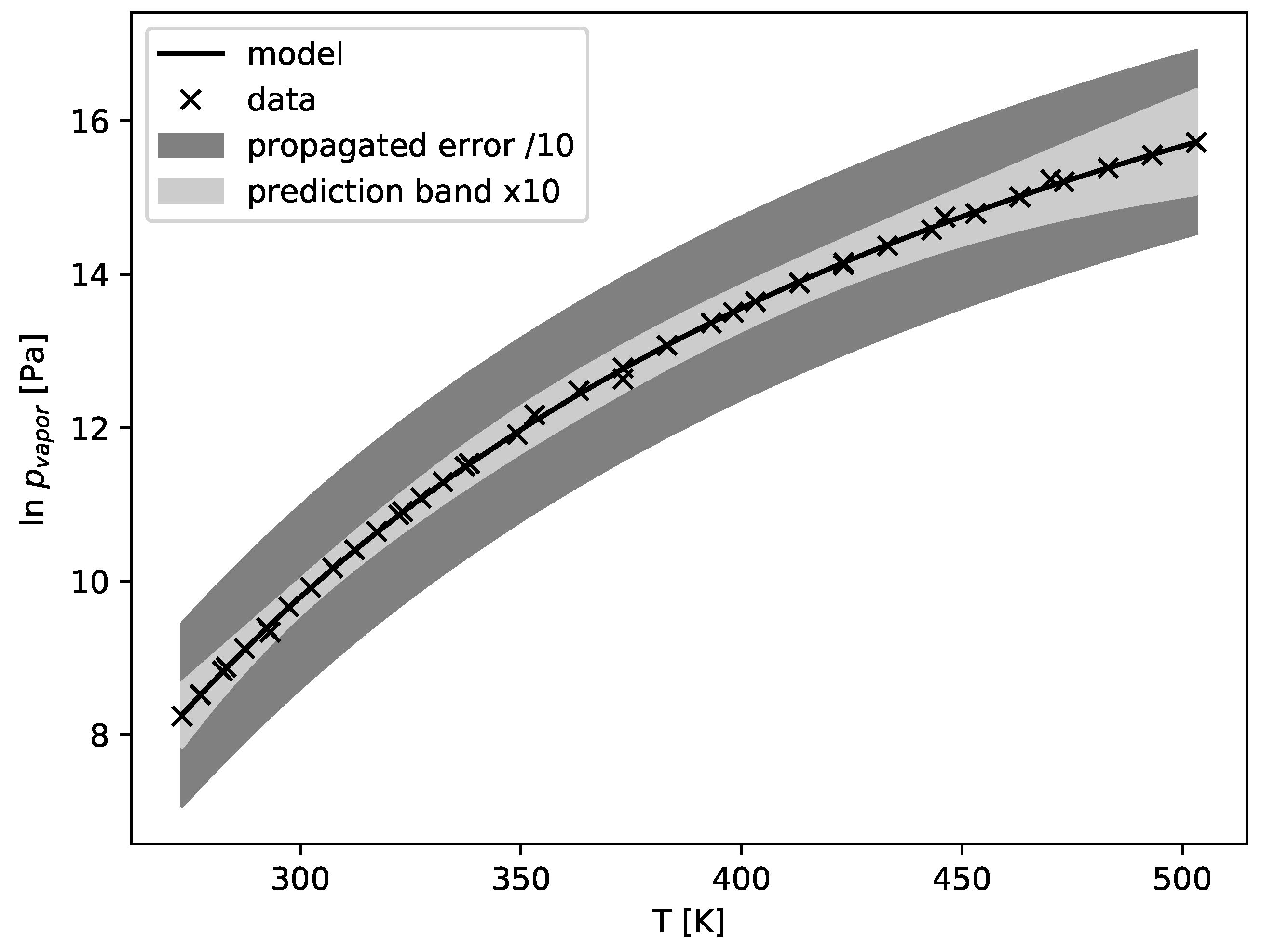
Figure 7, the area of the bounding box is much larger than the area of the ellipse itself. The behavior gets more pronounced in higher dimensions. This effect is demonstrated in
Figure 8 for the DIPPR model described in
Section 3.1 with three parameters. The prediction error band (Equation (
35)) is magnified ten times to be even visible, whereas the error propagation result (Equations (
34) and (
36)) is shrunk by the same factor to lie inside the plot. The error estimate based on the confidence intervals is more than 100 times larger than the prediction band. As a result, for error propagation of correlated models, the prediction band method [
23] should always be preferred over the simple propagation of confidence intervals.
However, the error propagation formulas in Equations (
36) and (
37) are useful, when various models are employed in one calculation. Different models are usually adjusted using different datasets and by multiple independent regression procedures. Assume, that
f,
g, and
h are models for three different properties of a system, e.g., vapor pressure, heat capacity, and activity coefficients for a binary mixture. Then, there may be a derived property that depends on all three of them
, and the error of
F resulting from all three parameter estimations is given by
If the parameters are correlated, Equation (
37) can be applied. Correlations are expected, e.g., if
f is used in the parameter estimation for
g or
h, e.g., to transform some of the input data. It is also possible to derive corresponding equations for cases where only some pairs are uncorrelated, by considering a covariance matrix where some off-diagonal elements are non-zero.
5.2. General Form of the Fisher Information Matrix
Thus far, the formula for the Fisher information matrix given in Equation (
32) is provided only for the single output case. However, it can be easily extended to the multiple output case, as long as every data point contains values for the output quantities. In process engineering, often multiple thermodynamic models are employed in a single calculation. We, therefore, present a strategy for treating such generalized situations in the parameter estimation process. When several inhomogeneous datasets are involved, this procedure is similar to missing-data problems [
33]. However, this approach does not aim to replace the missing data, but to use as many of the available data as possible.
First, consider
M models
, where
is the subset of input quantities that are used by the
ith model measured at the
jth data point. Models with multiple outputs are treated as multiple independent single-output models which have the same set of input quantities. Then, let
be the subset of
which contains all those data points, where all of the
and
are measured, or equivalently the set of data points that are useful for estimating the parameters of model
i. Then, the total model for the parameter estimation reads
The regression strategies given in
Section 2 can be generalized to this model. To that end, the numbers of inputs (
) and outputs (
) become dependent on the data point, but the equations provided are independent of this fact. The generalization of the Fisher matrix reads
where
denotes the corresponding standard deviation. A derivation based on probability theory is contained in
Appendix C.
Equation (
40) is fully additive with respect to the model functions and the data points. However, the formula contains the standard deviations of the measurements, which are rarely well-known. For the parameter estimation, approximate values might be sufficient in cases where the optimal parameters are not very sensitive to the standard deviations. For the error estimation, however, that is no longer true. Therefore, it is popular to estimate a common standard deviation
from the residual of the objective function,
, as done in Equation (
32). If the standard deviations of the dataset depend on the data points, then only a global scaling factor for all of them is estimated. The standard deviations
in Equation (
40), however, depend on the data point
j and the model
i. If just a single correction factor is estimated, the additivity of the Fisher matrix is violated, and the dependence of that factor on
N and
is not clear. For this reason, the re-estimation of the standard deviation is performed separately for each output using the corresponding number of data points and parameters.
Scaling the whole objective function by one (positive) scalar has no impact on the minimum value. This is no longer the case when different terms of the objective function are scaled by different factors, as in Equation (
40). The correct approach would be to iteratively solve for optimal parameters and estimate the standard deviations until self-consistency is reached. Assuming that the new estimates of the individual output errors do not change their ratios by large amounts, we use the first iteration as an approximation to the self-consistent one.
Another advantage of this approach is that the simultaneous regression of disjoint models on disjoint datasets yields the same result as two independent calculations.
6. Conclusions
Different strategies to address parameter estimation problems that are relevant to applications in process engineering in general and especially in thermodynamics have been discussed. The standard least-squares approach is useful for simple situations with a univariate regression problem and measurement errors in the outputs only, not in the inputs. Measurement errors in the inputs, however, lead to constrained least-squares problems, where the number of equality constraints grows with the number of measurement points. In this situation, the Patino–Leal formulation is a valuable alternative, since it transforms the constrained least-squares problem to a non-restricted optimization problem. We applied both methods to thermodynamic regression examples.
Furthermore, we demonstrated that, for multivariate parameter estimation or reconciliation problems, a multi-criteria approach yields substantial insight into how well a model can describe multiple responses at all. To the best of our knowledge, this is the first time that the challenge of reconciling process variables was treated within a multi-criteria setting. All the described algorithms were implemented with the industrial partners.
A direction for further research is, e.g., to realize the propagation of the parameter errors from thermodynamic models all the way up to a full flowsheet simulation of a real-world example. In addition, benchmarking of the various parameter estimation strategies should be performed applying them to more complex models.

 ,
, 


