Simulation of Conjugate Heat Transfer in Thermal Processes with Open Source CFD

Abstract

A verification and validation study was performed using the open source computational fluid dynamics software package OpenFOAM version 6-dev for conjugate heat transfer problems. The test cases had a growing complexity starting from a simple steady state problem over unsteady heat transfer to more realistic engineering applications. First, a fin effectiveness study was performed. Then, the external convection at pipes and internal pipe heat transfer were investigated. The validity of the techniques was shown for each test case by comparing the simulation results with experimental and analytic data available in the literature. Finally, a simplified shell-and-tube heat exchanger was simulated to demonstrate how these methods can be applied to plant scale engineering problems.

1. Introduction

Designing the process equipment for power or chemical plants is still based on empiricism or precedence, i.e., knowledge accumulated from prior experience. Due to inefficient designs, traditional resources (raw materials, hardware, utilities, and energy) are not exploited effectively, which leads to high production costs, a loss of product quality, and environmental pollution. An excellent review of the impact of a lack of process understanding on reliability and energy-efficiency, as well as safety was given by Joshi et al. [1,2].

The reason for the persistent high level of empiricism in process design is the complexity of heat and mass transfer in the process equipment. In general, the industrial equipment is operated at turbulent flow conditions, where vortical fluid motions (eddies) at different length and time scales contribute toward mixing and the transport of momentum, heat, and mass. A consistent modeling of such transport phenomena is a must to identify the relevant process parameters and will enable improvement in the scale- up and design procedures.

In recent years, some excellent reviews are provided for CFD in heat exchangers [3,4]. However, commercial software is predominantly used for most referenced simulations and not a single reference to the use of OpenFOAM is found in these reviews. The reason may be found in the lack of usability of existing multi-region solvers in OpenFOAM. Multi-region approaches are required, if the convective heat transfer from one fluid through a wall into another fluid is simulated.

There are many publications on heat transfer investigations using OpenFOAM, but they are often limited to the convective heat transfer in a single fluid region [5,6,7].

The published research using OpenFOAM for conjugate heat transfer simulations is often performed involving code modification, extension or re-implementation. Schremb et al. [8] studied the heat transfer due to an impinging droplet on a flat surface. A multiphase modeling approach is implemented in combination with the conjugate heat transfer methodology. The application of these modified solvers is often limited to benchmark. There are very few publications of conjugate heat transfer simulations with OpenFOAM that are applied to complex industrial equipment like real heat exchangers. Greiciunas et al. [9] simulate a compact plate-fin heat exchanger with serrated corrugation in cross flow orientation and compared the results with experimental data.

Very little research has been performed with the specific objective of testing and validating the conjugate heat transfer methods in OpenFOAM^® for fundamental problems. However, many researchers and users in the industry see a demand for constant validation and verification of these open-source CFD methods that are in constant development. Only for turbulent single phase flows without heat transfer several authors have published validation studies in recent years. In several publications, turbulence models in OpenFOAM^® were validated for the simulation of flows over bluff bodies [10,11,12].

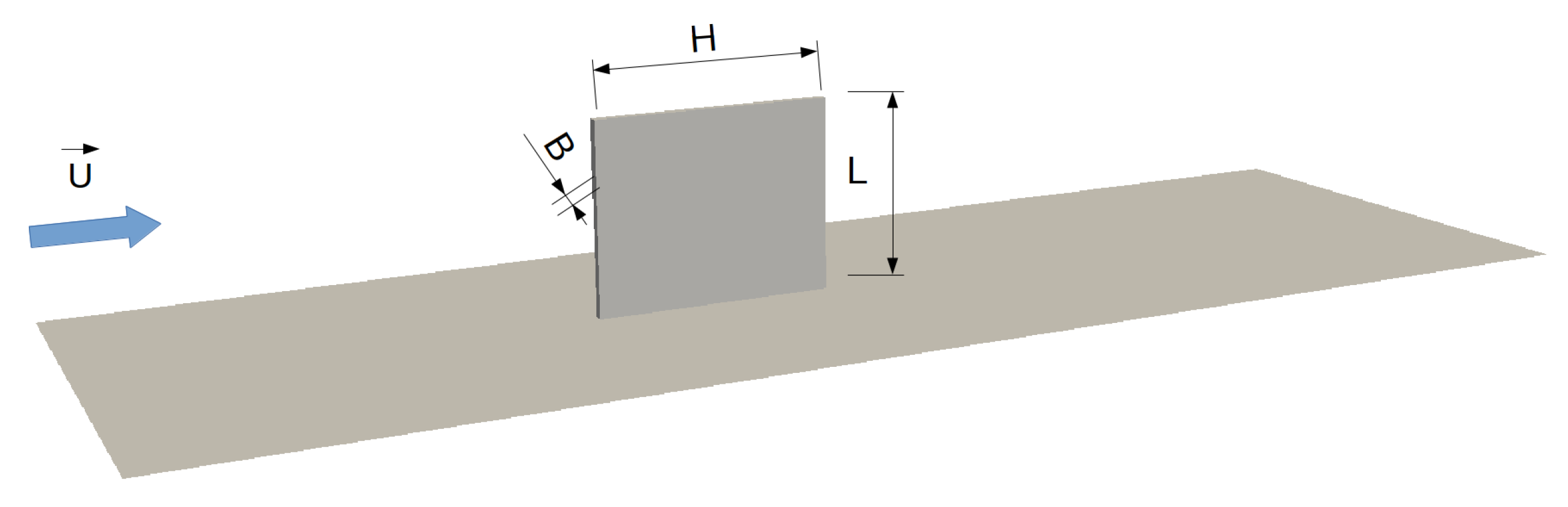
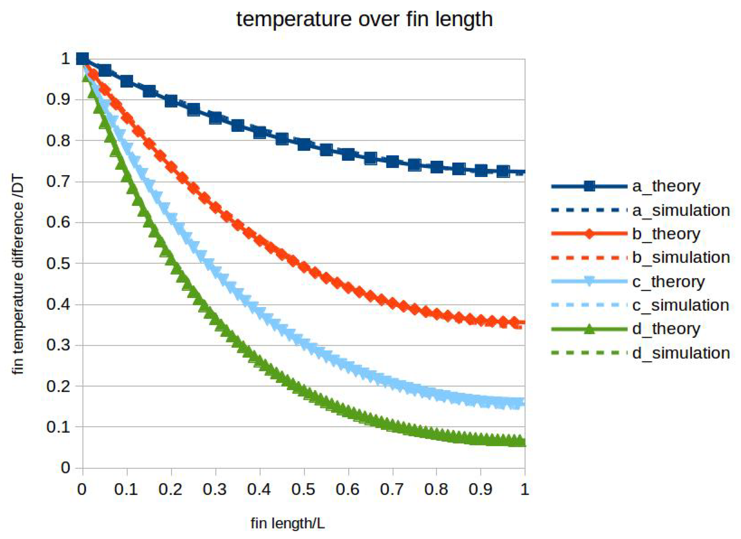
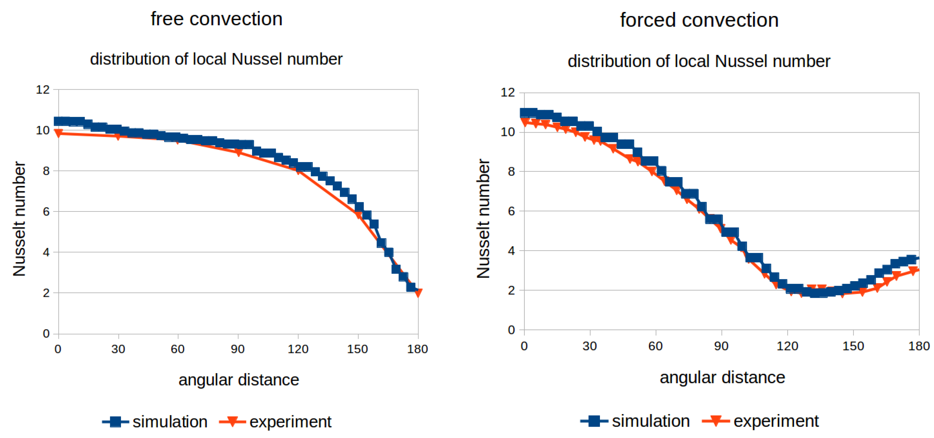
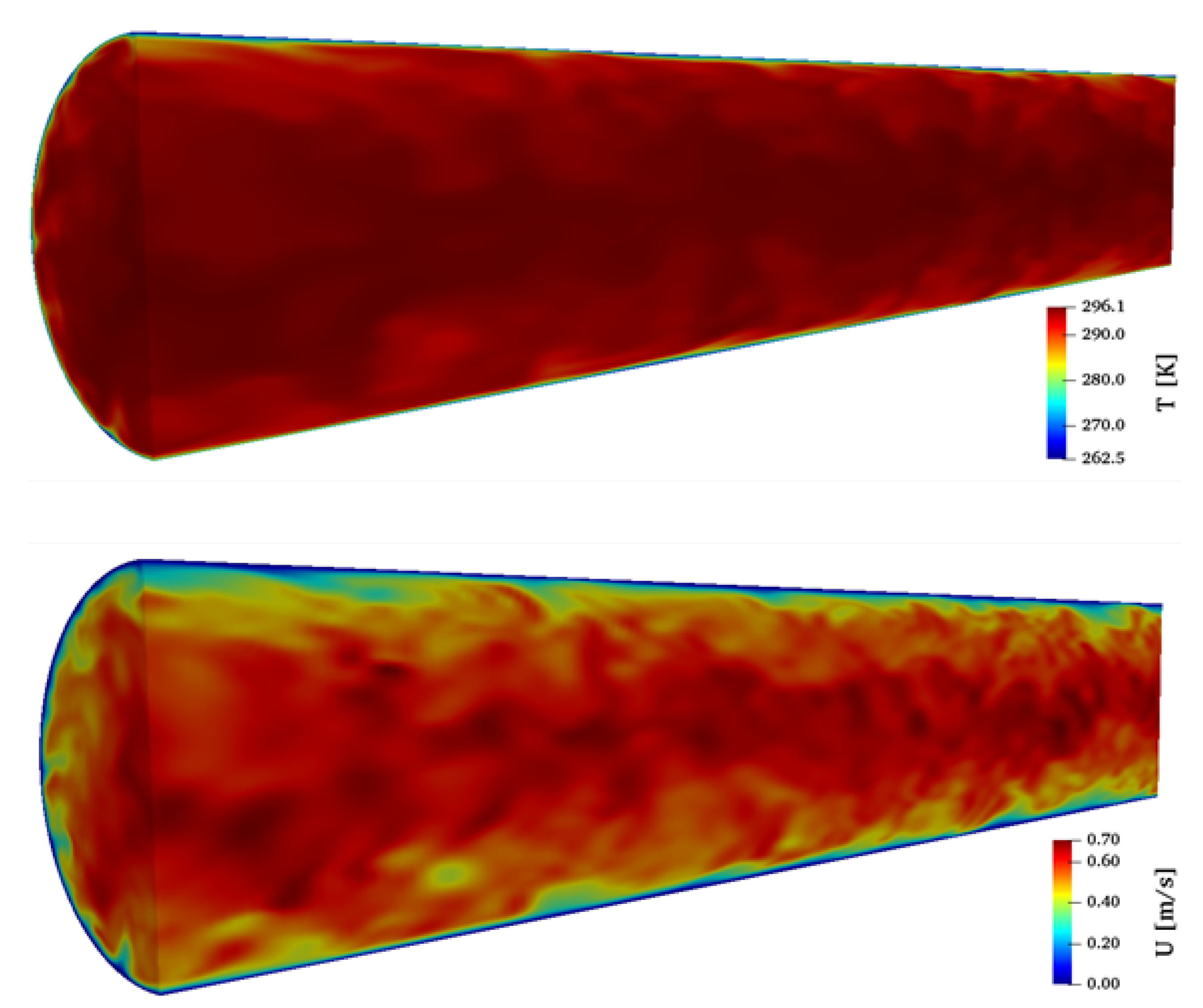
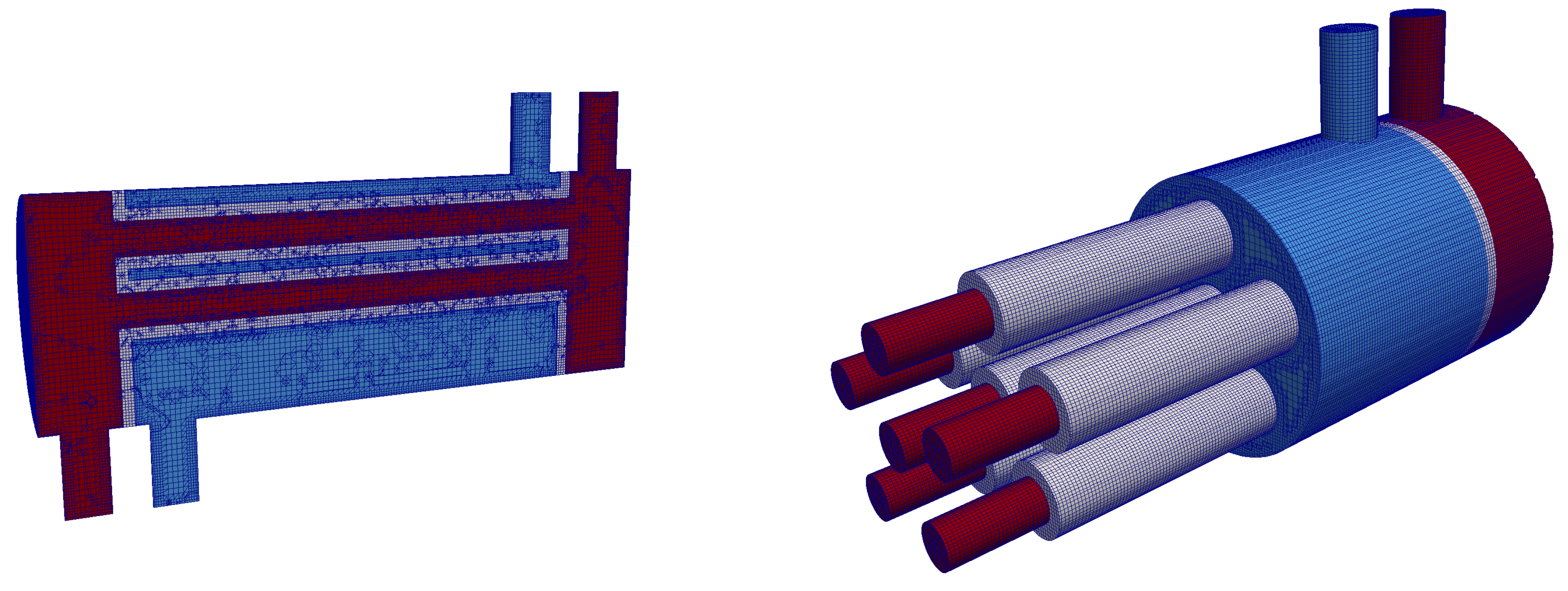
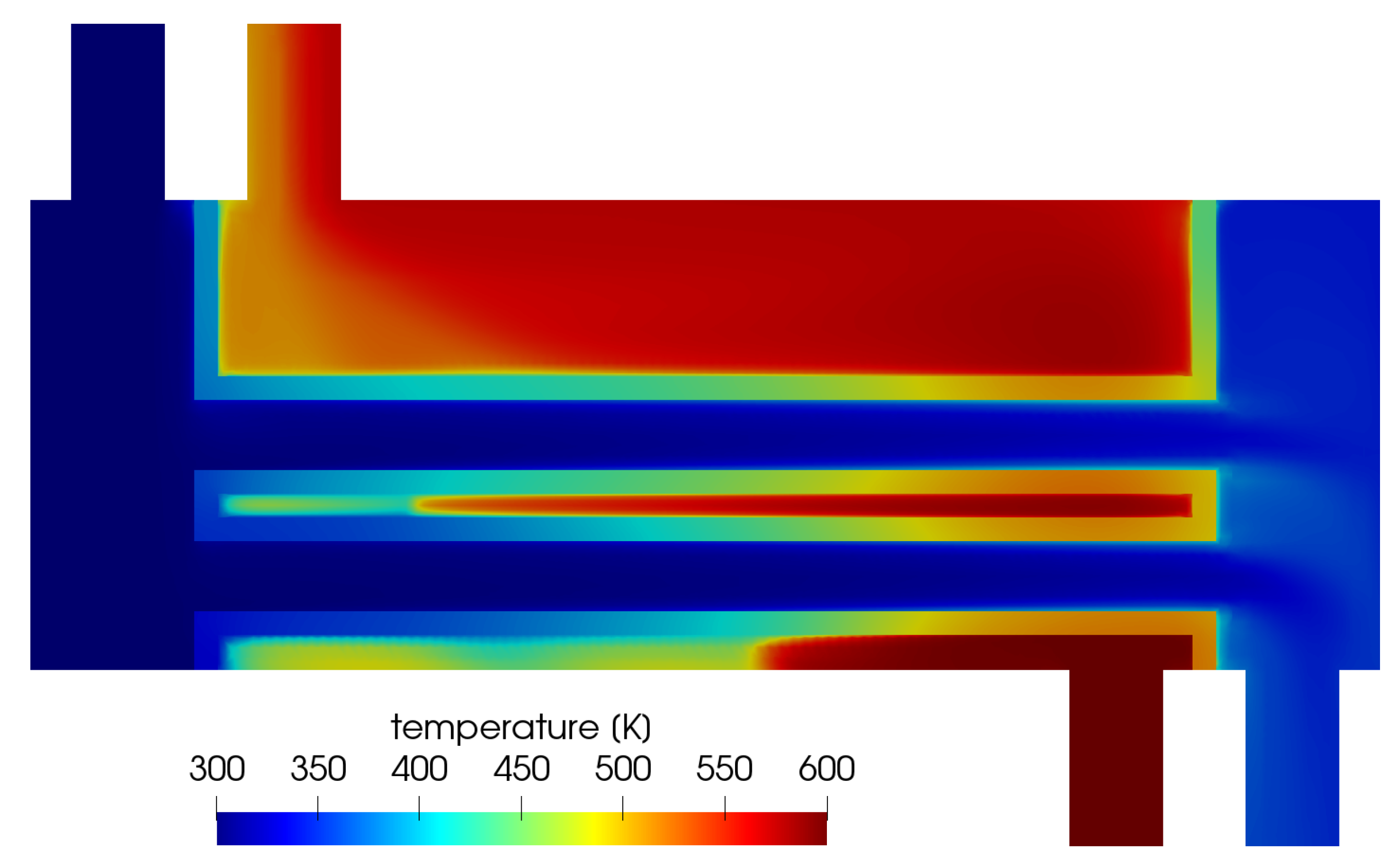
In the present study, a verification and validation study was performed using the open source computational fluid dynamics library OpenFOAM^® version 6-dev for conjugate heat transfer problems. The test cases had a growing complexity starting from a simple steady state problem over unsteady heat transfer to more realistic engineering applications. The applications were a fin effectiveness study, external convection at pipes, internal pipe heat transfer, and as a final example a simplified shell-and-tube heat exchanger. The validity of the techniques was shown for each test case by comparing the simulation results with experimental and analytical data available in the literature.

2. Physical Modeling

Today, heat transfer problems are often analyzed using a conjugate, coupled, or adjoint formulation. These three equivalent terms correspond to the problems containing two or more subdomains with phenomena described by different types of differential equations [13]. If the heat transfer in a solid body and a neighboring fluid is considered, the first is described by the Laplace equation and the latter by the Navier–Stokes equations. Thus, heat transfer through solid and fluid regions can always be considered as a conjugate problem.

The solution methodology used here was implemented in OpenFOAM^® (Open Source Field Operation and Manipulation). OpenFOAM^® is an object-oriented software library programmed in C++ and designed for the numerical solution of differential equations from continuum mechanics, as demonstrated by Jasak and Weller [14]. OpenFOAM^® is distributed with a variety of predesigned solvers. Usually, the finite volume method (FVM) is applied. Here, the edition OF6-dev was chosen with the solvers chtMultiRegionFoam and buoyantPimpleFoam. For the fluid regions, the solution algorithm in both solvers was identical. In the following, the governing equations are briefly described.

The physical modeling of flows with heat transfer is based on conservation laws for mass, momentum, and energy, as shown by Anderson [15]. The continuity equation for an unsteady flow of a compressible fluid can be formulated as

$$\frac{\partial \varrho }{\partial t}+\nabla ·\left(\varrho \mathbf{u}\right)=0$$

(1)

with the nabla-operator $\nabla =\left(\frac{\partial }{\partial x},\frac{\partial }{\partial y},\frac{\partial }{\partial z}\right)$, the density $\varrho$ and the velocity field $\mathbf{u}$.

The conservation of momentum is formulated as

$$\frac{\partial \left(\varrho \mathbf{u}\right)}{\partial t}+\nabla ·\left(\varrho \mathbf{u}\mathbf{u}\right)=-\nabla p+\varrho \mathbf{g}+\nabla ·\left(2{\mu }_{eff}\mathbf{S}\left(\mathbf{u}\right)\right)-\nabla \left(\frac{2}{3}{\mu }_{eff}\left(\nabla ·\mathbf{u}\right)\right),$$

(2)

where p is the static pressure field and g is the gravitational acceleration. The effective viscosity ${\mu }_{eff}$ is the sum of the molecular and turbulent viscosity. The rate of strain (deformation) tensor $\mathbf{S}\left(\mathbf{u}\right)$ is defined as $\mathbf{S}\left(\mathbf{u}\right)=\frac{1}{2}\left(\nabla \mathbf{u}+{(\nabla ·\mathbf{u})}^T\right)$.

The conservation of energy in the fluid is defined in terms of the specific enthalpy h as

$$\frac{\partial \left(\varrho h\right)}{\partial t}+\nabla ·\left(\varrho \mathbf{u}h\right)+\frac{\partial \left(\varrho k\right)}{\partial t}+\nabla ·\left(\varrho \mathbf{u}k\right)-\frac{\partial p}{\partial t}=\nabla ·\left({\alpha }_{eff}\nabla h\right)+\varrho \mathbf{u}·\mathbf{g},$$

(3)

where $k={\left|\mathbf{u}\right|}^2/2$ is the specific turbulent kinetic energy. The effective thermal diffusivity ${\alpha }_{eff}$ is the sum of laminar and turbulent thermal diffusivities

$${\alpha }_{eff}=\frac{\varrho {\nu }_t}{P{r}_t}+\frac{\mu }{Pr}=\frac{\varrho {\nu }_t}{P{r}_t}+\frac{k_f}{c_p},$$

(4)

where $k_f$ is the thermal conductivity, $c_p$ is the specific heat at constant pressure, $P{r}_{(t)}$ is the (turbulent) Prandtl number and ${\nu }_{(t)}$ is the (turbulent) kinematic viscosity. The equations for the hydrodynamics and thermodynamics of the fluid flow (Equations (1)–(4)) are extended to include energy transport due to transient heat conduction within the solid wall according to

$${\varrho }_s{c}_s\frac{\partial T_s}{\partial t}=\nabla ·\left(k_s\nabla T_s\right).$$

(5)

The turbulent transport parameters in Equations (1)–(4) require a turbulence closure with a corresponding modeling technique.

In three of the later four reference cases, the k-Omega-SST model was chosen. This includes two additional transport equations to represent turbulent properties of the flow: the transport of kinetic energy k and the scale of the turbulence $\omega$. The extended SST (shear stress transport) model is known for its good behavior in adverse pressure gradients and separating flows [16].

Recently, tensor-based models are applied more often. A thorough discussion is not possible here, but recent improvement has been made in RANS-development such as the v2-f-model [17,18] or the scale-adaptive model [19]. In recent years, the effort for the development of RANS models has been strongly reduced due to lack of general success as well as the rapidly increasing computational resources that allow the application of more costly methods. Therefore, in one of the following test cases, the LES technique was applied, i.e., only the large-scale vortices that contain most of the turbulent kinetic energy were directly resolved and all smaller scale vortices were modeled [20,21]. Similarly, the accuracy compared to RANS was increased substantially and at the same time the numerical effort compared to DNS was reduced up to a level that makes this approach interesting for the industry. A detailed overview about the LES techniques is given in [22].

These techniques have been demonstrated to perform well for technically relevant turbulent flows [23,24,25]. In LES, a filter function with a characteristic filter width $\Delta$ is applied to Equations (1)–(3), so that the field variables are decomposed into a resolved and a non-resolved part. Thus, the velocity vector becomes $\mathbf{u}=\widehat{\mathbf{u}}+{\mathbf{u}}^{\prime }$. The expression for the effective viscosity is reformulated to ${\nu }_{eff}=\nu +{\nu }_{SGS}$, i.e., the sum of molecular and apparent viscosity of the subgrid scales. Following the Boussinesq approximation, the subgrid scale viscosity is then modeled as ${\nu }_{SGS}=C_k\Delta \sqrt{k_{SGS}}$ with $C_k=0.07$ and $k_{SGS}$ as the kinetic energy of the subgrid scales. The Smagorinsky model [20] utilizes a simple diffusion model for this

$$k_{SGS}=2\frac{C_k}{C_{ϵ}}{\Delta }^2{\left|\mathbf{S}\right|}^2,$$

(6)

with $C_{ϵ}=1.048$ and $\left|\mathbf{S}\right|={(\mathbf{S}:\mathbf{S})}^{1/2}$.

In the current work, the so-called WALE (Wall-Adapting Local Eddy-viscosity) model was applied [26]. The subgrid scale viscosity was calculated in the same way as shown above, but the calculation of the subgrid scale kinetic energy was slightly different:

$$k_{SGS}={\left(\frac{C_w^2\Delta }{C_k}\right)}^2\frac{{\left(S_{ij}^d{S}_{ij}^d\right)}^3}{{\left({\left({\overline{S}}_{ij}{\overline{S}}_{ij}\right)}^{5/2}+{\left(S_{ij}^d{S}_{ij}^d\right)}^{5/4}\right)}^2},$$

(7)

with $C_w=0.325$ and $C_k=0.094$. Thus, this model takes into account the rotation of the flow field for the calculation of $k_{SGS}$ and it can be applied without additional damping for ${\nu }_{SGS}$ in the near wall region.

3. Results

3.1. Investigation of Fin Effectiveness

First, the heat transfer through a straight and regular steel fin was investigated. Fins are surfaces that extend into the flow. In heat transfer equipment, the purpose of the fin is to increase the product of the surface area and the heat transfer coefficient [27]. The design of the heat exchanger is dependent on the knowledge about the actual fin efficiency. The efficiency of a fin is defined as the ratio of the actual heat transfer from the fin to the heat that would be dissipated if the whole surface of the fin is kept at constant base temperature. With increasing length of the fin, the resistance to the heat conduction increases and the effectiveness decreases. Numerous experiments have been performed in the past on this subject. Goldstein and Sparrow [28] determined the heat transfer coefficient by using the heat and mass transfer analogy. Hatada et al. [29] and Kang and Kim [30] tested the actual heat exchangers in a wind tunnel. Here, the OpenFOAM^® solver chtMultiRegionFoam was applied to simulate fin effectiveness.

3.1.1. Numerical Set-Up of the Fin Test Case

A regular straight fin was investigated. The computational domain is depicted in Figure 1. At the base of the fin, the temperature was kept constant at $T_{base}=363$ K. The fin iswas cooled by a turbulent airflow at ambient conditions ($p_a=1$ bar, $T_a=300$ K). Several simulations were performed at different fin lengths $L=0.02$–$0.08$ m. The air was treated as perfect gas and the material of the fin was steel with constant thermodynamic properties. The case was simulated as steady state with the kOmegaSST turbulence model to account for the turbulence of the air flow.

Figure 1. Schematic representation of the computational domain of the fin investigation.

In Table 1, an overview of the parameters of the simulation set-up is given. It includes the thermodynamic properties of the materials, flow conditions and geometrical data.

Table 1. Parameters of the fin simulation set-up.

Parameter	Variable	Unit	Value
fin length	L	m	(a) $0.02$; (b) $0.04$; (c) $0.06$; (d) $0.08$
fin thickness	B	m	$0.002$
fin height	H	m	$0.05$
fin temperature at base	$T_{base}$	K	363
density of steel	${\varrho }_s$	kg/m${}^3$	7850
heat capacity of steel	$c_s$	J/(kgK)	645
thermodynamic conductivity of steel	$k_s$	W/(mK)	40
size of computational domain	$X,Y,Z$	m	$0.3,0.1,0.1$
air temperature at inlet	$T_a$	K	300
air pressure at outlet	$p_a$	bar	1
air Prandtl number	$Pr$	-	$0.7$
air turbulent Prandtl number	$P{r}_t$	-	$0.9$
air inlet velocity	$u_a$	m/s	10
air Reynolds number	$R{e}_a=\frac{{\varrho }_a{u}_{a}H}{{\eta }_a}$	-	32,262

In Figure 2, the numerical grid and the temperature contours of the fin for the simulation case (b) (L = 0.04 m) are depicted in an exemplary manner. Along the length of the fin, the temperature quickly decreased from base level down to $T=325$ K. The coolest spot on the fin was clearly visible at the upstream fin corner, because it was at maximum distance from the fin base, the surrounding air temperature was at a minimum and the local heat transfer near the sharp edge is high. Towards the downstream fin corner, the temperature increased as the surrounding air temperature became higher.

Figure 2. (left) Numerical grid in fluid and solid block; and (right) temperature contours along solid and fluid patches as well in a cross section for Simulation Case (b) L = 0.04 m.

3.1.2. Results of the Fin Test Case

The theoretical fin effectiveness ${\eta }_{th}$ can be derived from the assumption of thermal equilibrium at the fin [31]. It is

$${\eta }_{th}=\frac{{\dot{Q}}_{\mathrm{actual}}}{{\dot{Q}}_{\mathrm{ideal}}}=\frac{\mathrm{actual} \mathrm{heat} \mathrm{transfer}}{\mathrm{maximum} \mathrm{possible} \mathrm{heat} \mathrm{transfer}}.$$

(8)

This equation becomes

$${\eta }_{th}=\frac{\underset{0}{\overset{L}{\int }}h·\Delta T_{(x)}·U·dx}{h·\Delta T_1·U·L}=\frac{tanh(m·L)}{m·L},$$

(9)

where h is the overall heat transfer coefficient, L the fin length and the parameter m is

$$m=\sqrt{\frac{h·U}{k_s·A}}.$$

(10)

Here, U is the circumference, A the cross section ($B·H)$ and $k_s$ the thermal conductivity of the fin.

In Table 2, the theoretical film effectiveness ${\eta }_{th}$ is presented for Simulation Cases (a)–(d), i.e., $L=0.02$–$0.08$ m. Then, ${\eta }_{th}$ is juxtaposed with the simulated film effectiveness ${\eta }_{sim}$ from the CFD simulations. The overall agreement is very good considering that the theory values neglect all non-idealities such as non-uniformity of the boundary layers, non-uniform heat transfer coefficient and non-uniform temperature field along the fin.

Table 2. Comparison of the theoretical and the simulated film effectiveness.

Case	(a)	(b)	(c)	(d)
L	$0.02$ m	$0.04$ m	$0.06$ m	$0.08$ m
${\eta }_{th}$	0.800	0.545	0.385	0.294
${\eta }_{sim}$	0.814	0.552	0.389	0.295

Following the same theory as above, the theoretical local temperature profiles along the fin can be calculated with

$$\Delta T(x)=\Delta T_1·\frac{cosh(m·(L-x))}{cosh(m·L)}.$$

(11)

with $\Delta T_1=T_{base}-T_a$ and x the coordinate along the fin length. In Figure 3, these profiles are juxtaposed to the simulation results for each case. The temperature was made dimensionless with $\Delta T_1$ and the dimensionless coordinate $x/L$ was chosen. The agreement in the local temperature field between the theory and the simulation data is very good considering the above mentioned non-idealities.

Figure 3. Temperature profiles along the fin for different simulation cases compared to theory; solid lines and symbols: theory; dashed lines: simulation data.

3.2. External Heat Transfer at Pipes with RANS Approach

Next, the application of the conjugate heat transfer capabilities of OpenFOAM were demonstrated for external cooling of a water pipe flow with air. Again, the reference simulations were carried out and the results compared to literature data.

3.2.1. Numerical Set-Up of External Pipe Test Case

The computational domain is depicted in Figure 4. This quasi-two-dimensional case consists of the hot water region inside the pipe, a copper pipe region and the region of the cool surrounding air. The simulation includes the convective heat transfer from water to the copper pipe, the heat conduction through the pipe and the convective heat transfer from the pipe outside to the surrounding air. In the first step, only natural convection was considered at the pipe outside. In the second step, a forced convection at laminar flow conditions was considered at the pipe outside. The air was treated as perfect gas and water as perfect fluid. The thermodynamic properties of the solid region corresponded to copper and were constant. Both cases were obviously unsteady. In Table 3, an overview of the parameters of the simulation set-up is given for both reference cases.

Figure 4. Computational grid of the water, copper and air region: (left) whole computational domain; and (right) mesh in the vicinity of the pipe.

Table 3. Parameters of the external pipe flow simulation set-up.

Parameter	Variable	Unit	Value
pipe inner diameter	$d_i$	m	$0.0283$
pipe outer diameter	$d_o$	m	$0.0442$
pipe length	$L_p$	m	$0.0884$
size of air domain	$X,Y,Z$	m	$0.8,1.4,0.0884$
natural convection reference case:
water temperature	$T_w$	K	315
water velocity	$u_w$	m/s	5
air temperature	$T_a$	K	300
air Prandtl number	$P{r}_a$	-	$0.7$
Raleigh number	$Ra$	-	$0.86\times {10}^5$
forced convection reference case:
water temperature	$T_w$	K	330
water velocity	$u_w$	m/s	5
air temperature	$T_a$	K	300
air Prandtl number	$P{r}_a$	-	$0.7$
air velocity	$u_a$	m/s	$0.0489$
Reynolds number	$R{e}_D$	-	130

The numerical grid used for this reference case is displayed in Figure 4. In Figure 4 (left), the whole computational domain is shown, and in Figure 4 (right) the vicinity of the pipe is enlarged. All three regions are labeled correspondingly. The total number of grid cells was about 133k for the air region, 8k for the copper region and 8k for the water region. The simulations were carried out on four CPU cores only. The time step size was about $\Delta t=0.001$ s for all simulations and the total simulated time was $t_t=50$ s for all cases.

3.2.2. Results of the External Pipe Test Case

In Figure 5 (left), temperature contours are shown for the case of free convection cooling at a Raleigh number of $Ra=0.86\times {10}^5$. It is clearly visible that the heat flux from the inner pipe flow was transferred to the surrounding air. The air around the pipe was heated and due to the density difference a convective flow was induced. The hot air rose from the pipe in the form of a laminar plume. That plume was stable up to a few pipe diameters above the pipe, then instabilities evolved and the plume broke up.

Figure 5. Temperature contours in a cross section: (left) free convection; and (right) forced convection.

In Figure 5 (right), temperature contours are shown for the case of a forced convection test case at a low laminar Reynolds number of $R{e}_D=130$. At this flow regime, a classical Kármán vortex street developed in the wake behind the pipe. The heat was transferred from the inner pipe through the copper solid material to the surround air flow. The temperature contours in the wake emphasized the vortex street vortical structures.

In Figure 6 (left), the simulation results of the free convection test case are compared to experimental data [32]. The distribution of the local Nusselt number is shown around the pipe and and plotted over the angular coordinate starting with zero at the upstream stagnation point. At $0^{\circ }$, the heat transfer was at a maximum and declined with increasing angular coordinate down to the hot wake. The simulation results match the experiments very well.

Figure 6. Comparison of the local Nusselt number distribution between literature data and simulation data: (left) free convection, experimental data from [32]; and (right) forced convection, experimental data from [33].

In Figure 6 (right), the simulation results of the forced convection test case are compared to experimental data [33]. Again, the distribution of the local Nusselt number is shown around the pipe and and plotted over the angular coordinate starting with zero at the upstream stagnation point. At $0^{\circ }$, the heat transfer was at a maximum and declined with increasing angular coordinate. Around ${120}^{\circ }$, the minimum was reached. After that, the heat transfer was again slightly increasing due to the oscillating wake movement. The simulation results match the experiments very well. Thus, it was shown that it is not only possible to predict global heat transfer for steady state cases, but local phenomena at unsteady cases can also be simulated with a reasonable accuracy that is sufficient for many engineering purposes.

3.3. Turbulent Heat Transfer of Internal Pipe Flow Using LES

In the previous two experiments, the conjugate heat transfer solvers of OpenFOAM^® were validated for steady state and transient heat transfer problems. However, in both cases, the heat transfer limitation was at the low Prandtl number flow around a certain geometry. This could be calculated with standard RANS models relatively easily. More difficult was the prediction of heat transfer of internal flows in process equipment with moderate or high Prandtl numbers. This section shows that the turbulence modeling techniques in OpenFOAM^® can be applied for such problem with equal success. As a reference case, a simple turbulent pipe flow with heat transfer was chosen.

3.3.1. Numerical Set-Up of the Internal Pipe Flow Test Case

The accurate calculation of heat transfer in turbulent pipe flow required a fully developed turbulent flow inside the pipe. Usually, limitations of computational resources did not allow simulations of a long pipe to ensure a fully developed flow. By simulating a small section of a pipe with periodic boundary conditions at the inlet and outlet, a fully developed turbulent flow could also be achieved if a sufficient number of flow cycles were carried out.

Therefore, the simulations of the present work were done in a smooth pipe with a length of $L=6d$ in streamwise direction, where d is the diameter of the pipe. A schematic representation of the computational domain is shown in Figure 7. The hexagonal structured grid of the computational domain had a total number of about 2.8 million cells, and, to resolve the near-wall region, the sufficiently accurate grid cell size was stretched in radial direction. This led to the first grid point $y_1^{+}$ being located within the viscous sublayer for each simulation. Characteristic quantities of the numerical grids and simulation parameters of the present simulations are summarized in Table 4. Due to the high resolution of the grid, the simulations required a high computing power and were performed each on 84 CPUs on a high performance computing cluster (HPC-Cluster).

Figure 7. Schematic representation of the computational domain. The coordinate system is given as $r,x,\omega$.

Table 4. Simulation parameters of the present LES.

$\mathit{Re}=({\mathit{U}}_{\mathit{m}}{\mathit{d}}_{\mathit{h}})/\mathit{\nu }$	8000	8000	8000	16,000
Pr	5	7	9	7
${\mathit{y}}_{\mathbf{1}}^{+};\Delta {\mathit{r}}_{\mathit{min}}^{+}$	0.05	0.051	0.052	0.09
$\Delta {\mathit{\omega }}_{\mathit{max}}^{+}$	9.2	9.1	9.2	16.2
$\Delta {\mathit{x}}^{+}$	18.5	18.2	18.5	32.5
${\mathit{Re}}_{\mathit{\tau }}=({\mathit{U}}_{\mathit{\tau }}{\mathit{d}}_{\mathit{h}})/\mathit{\nu }$	520	509	514	909

In axial direction, cyclic boundary conditions were applied and, to maintain an average flow velocity, a source term was added to the momentum equation that adjusted the velocity to the desired value. A no slip boundary condition was applied to the pipe wall and a constant temperature gradient of ${\delta T/\delta r|}_w=-{10}^5$ K/m was used to take heat transport into account. By adding a uniform distributed internal heat source ${\dot{q}}_s$, which had the same amount as the resulting heat flux on the pipe wall ${\dot{q}}_w$, the temperature of the turbulent flow was kept at a constant level. To model the subgrid scales in the current large eddy simulations, the WALE (wall-adapting local eddy-viscosity) turbulence model was chosen [26].

The simulations were carried out with three different Prandtl numbers (5, 7 and 9) for a Reynolds number of $Re=8000$ and with one Prandtl number (7) for $Re=$ 16,000. Each simulation ran for a sufficiently long time to reach a fully turbulent flow. Afterwards, the statistics were gathered over a period of at least 20 through-flows of the computational domain, at 56 locations along the pipe. For reasons of stability and accuracy, the CFL number was kept equal or less than $0.3$ in each simulation.

3.3.2. Results of the Internal Pipe Flow Test Case

In this section, the results of the internal pipe flow simulations are presented. First, the used approach was validated to ensure that the simulations predict turbulent pipe flow correctly. Then, the results of the heat transfer evaluations are shown. In Figure 8, the 3D flow field of the computational domain is depicted.

Figure 8. Contours of the flow and temperature field at an instantaneous time step, $Re=8000$, $Pr=7$: (top) temperature; and (bottom) magnitude of velocity.

Mean Velocity Profiles and Root Mean Square Fluctuations

The mean axial velocity distributions normalized by the friction velocity $U_{\tau }$ versus the dimensionless distance from the wall $y^{+}$ are depicted in Figure 9 for $Pr=7$, $Re=8000$ and $Re=$ 16,000. For validation purposes, the present LES results were compared to the logarithmic law of the wall and to DNS results of Wagner et al. (2001) [34]. For both Reynolds numbers, the viscous sublayer region ($0<y^{+}<5$) was well resolved and matched the logarithmic law as well as the results of Wagner et al. (2001) [34]. The dimensionless velocity profiles in the buffer layer ($5<y^{+}<30$) and the logarithmic region ($y^{+}>30$) slightly deviate from the logarithmic law but they are in a good agreement with the DNS results.

Figure 9. Mean streamwise dimensionless velocity profile, $Pr=7$.

In Figure 10, the axial profiles of the root mean square velocity fluctuations scaled by the friction velocity $U_{\tau }$ versus the radial position normalized by the pipe radius R are shown for $Re=8000$ and $Re=$ 16,000. The validation was achieved by comparing the turbulent fluctuations of the present LES to the DNS results of Wagner [34]. The velocity fluctuations matched very well the DNS data. However, with distance to the wall, the velocity fluctuations ${\left(U_z^{+}\right)}_{rms}$ for $Re=8000$ were slightly underestimated compared to the DNS. The fluctuations ${\left(U_r^{+}\right)}_{rms}$ and ${\left(U_{\omega }^{+}\right)}_{rms}$ showed good agreement along the whole profile. The peak of the root mean square velocity fluctuations in axial direction ${\left(U_z^{+}\right)}_{rms}$ showed a noticeable increase with the Reynolds number, while the maximum of ${\left(U_r^{+}\right)}_{rms}$ and ${\left(U_{\omega }^{+}\right)}_{rms}$ were increased only slightly at the higher Reynolds number. Furthermore, the location of the peak of ${\left(U_z^{+}\right)}_{rms}$ was approaching the wall. The same behavior was also observed for the LES by Ould-Rouiss [35], who investigated turbulent pipe flow for various Reynolds and Prandtl numbers.

Figure 10. Mean streamwise velocity fluctuations, $Pr=7$.

When the Reynolds number increased, the turbulence strength increased and the thickness of the viscous sublayer ${\delta }_s$ decreased. With a near-wall grid resolution in radial direction for each simulation of $y_1^{+}<0.1$, it was ensured that the near-wall region was resolved sufficient.

Mean Temperature Profiles

The mean temperature profiles normalized by the friction temperature $T_{\tau }$ ($T_{\tau }=q_w/(\varrho c_p{U}_{\tau })$) as a function of the dimensionless distance $y^{+}$ are depicted for $Re=8000$ and $Pr=5,7,9$ in Figure 11. These profiles were compared with the correlations derived by Kader [36]. The present simulation results of the mean temperature show the typical curve shape and agree well with the theoretical law. For each Prandtl-number, the mean temperature profile of the viscous sublayer and the buffer region were consistent with Kader’s correlation. Only in the logarithmic region the results of the present LES were slightly overestimated and differed from the theory.

Figure 11. Mean resolved temperature profile, Re = 8000.

Heat Transfer Analysis

Due to the uniform internal heat source ${\dot{q}}_s$, the temperature was kept at a constant level while gathering the statistics. The resulting temperatures of the flow and the wall are shown for $Re=8000$ and $Pr=5$ in Figure 12. In this figure, the average temperature at the inlet and the wall temperature are depicted as a function of time. Averaging the temperatures in time led to the mean average temperatures at the inlet ${\overline{T}}_{ave,in}$ and the pipe wall ${\overline{T}}_{ave,wall}$. With the temperature difference $\Delta T={\overline{T}}_{ave,in}-{\overline{T}}_{ave,wall}$ and the known heat flux at the wall ${\dot{q}}_s$, the heat transfer coefficient could be determined. The resulting Nusselt numbers $N{u}_{simulation}$ for each simulation are summarized in Table 5. For validation purposes, the Nusselt numbers analytically calculated with the correlations of Gnielinski are also listed in this table [37]. The Nusselt numbers of the present simulations were slightly lower compared to the values determined analytically. However, with a deviation of less than 5% for the low Reynolds number and less than 10% for the high Reynolds number, the present calculations of the heat transfer in turbulent pipe flow showed a high accuracy.

Figure 12. Averaged temperatures at inlet and pipe wall, $Re=8000$ and $Pr=5$.

Table 5. Simulation parameters of the present LES.

$\mathit{Re}=({\mathit{U}}_{\mathit{m}}{\mathit{d}}_{\mathit{h}})/\mathit{\nu }$	8000	8000	8000	16,000
Pr	5	7	9	7
${\mathit{Nu}}_{\mathit{simulation}}$	59.3	69.3	73.5	116.0
${\mathit{Nu}}_{\mathit{Gnielinski}}$	61.9	70.2	77.0	128.0

3.4. Shell-And-Tube Heat Exchanger Test Case

As a last example, a complete shell-and-tube heat exchanger was simulated. This example is provided in the tutorial section of the current development version of OpenFOAM^®. Automated scripts are provided for the whole meshing, pre-processing and simulation steps. The example is shown here to demonstrate that the techniques described above can be applied to real process equipment and can be successfully used in the industry. The shell-and-tube heat exchanger was operated in counter-flow configuration. For reasons of simplicity, water was considered for both fluids. The mass flow for both fluids was the same and the thermodynamic properties were assumed constant. The material properties of the heat exchanger itself corresponded to aluminum. The parameters of the heat exchanger and the flow data are given in Table 6.

Table 6. Parameters of the external pipe flow simulation set-up.

Parameter	Variable	Unit	Value
mass flow rate	$\dot{m}$	kg/s	$0.05$
hot inlet temperature	${\theta }_1^{\prime }$	K	600
cold inlet temperature	${\theta }_2^{\prime }$	K	300
heat capacity	c	J/(kgK)	4181
Prandtl number	$Pr$	-	$6.62$
heat exchanger parameters
number of pipes	n	-	5
length of pipes	$L_p$	m	$0.174$
inner diameter of pipes	$D_p$	m	$0.012$
outer diameter of pipes	$P{r}_a$	-	$0.02$
total heat transfer area	$A_{HTX}$	m${}^2$	$0.044$

3.4.1. Numerical Set-Up of the Shell-and-Tube Heat Exchanger Test Case

In Figure 13, the computational grid of the shell-and-tube heat exchanger is shown. It was generated automatically with snappyHexMesh. In Figure 13 (left), a cut through of all regions (shell, tube, and solid) at the symmetry plane is depicted. Figure 13 (right) depicts cuts that were made in the axial direction for each region at a different axial position. The grid was generated with an automated script delivered with the solver. The only necessary input were the surface geometries in stereo-lithography (STL) format.

Figure 13. Computational grid of the shell-and-tube heat exchanger that was generated with snappyHexMesh: (left) cut through all regions (shell, tube, solid) at middle section; and (right) cuts in axial direction for each region at a different axial position.

The solver chtMultiRegionFoam was used with steady state configuration and the standard k-Epsilon model was applied to account for turbulence.

3.4.2. Results of the Shell-and-Tube Heat Exchanger Test Case

The simulation results were compared with engineering correlations [37] by means of the prediction of the overall heat flux only. First, the overall heat transfer coefficient was roughly estimated with the Nusselt number of the internal pipe flow, because it is the limiting heat resistance

$$N{u}_D\approx 0.0235·R{e}_d^{0,8}·P{r}^{0,48}=15.33.$$

(12)

Then the NTU method [38] is chosen to calculate the number of transfer units

$$NT{U}_1=\frac{h·A_{HTX}}{\dot{m}·c}=0.17.$$

(13)

With the $NT{U}_1$ value for fluid 1 (hot side), the dimensionless temperature $P_1$ is determined by means of an NTU diagram [37] for an ideal counter-flow heat exchanger. With the value for $P_1$

$$P_1=\frac{{\theta }_1^{\prime }-{\theta }_1^{″}}{{\theta }_1^{\prime }-{\theta }_2^{\prime }}$$

(14)

the outflow temperature of fluid 1 ${\theta }_1^{″}$ was calculated, which led to the overall heat flux with ${\dot{Q}}_1=\dot{m}c\left({\theta }_1^{\prime }-{\theta }_1^{″}\right)$.

Thus, the overall heat flux through the heat exchanger was estimated to be ${\dot{Q}}_1=9.4$ kW. The simulated heat flux from the simulation was ${\dot{Q}}_{sim}=10.5$ kW. The difference between the rough estimation and the simulation was around 5%. This is a very short verification of the techniques for automated meshing and simulation of a complete heat exchanger. Its intention is to show that the method is suitable for practical purposes.

In Figure 14, the temperature field is shown in the symmetry plane of the heat exchanger in all regions. The advantage of the numerical simulation of a total heat exchanger became evident, i.e., local hot spots and cool spots could be identified as well as the mal distribution of flow in the fluid regions. Here, the highest wall temperatures of the pipes were near the hot shell side inlet and the lowest pipe temperatures were near the cool tube side inlet, as was to be expected for a counter-flow heat exchanger. However, for a more complex heat exchanger, this prediction is of high interest for the design and operation and CFD simulations can deliver useful answers, as demonstrated here.

Figure 14. Temperature profiles along the fin for different simulation cases compared to theory; solid lines and symbols: theory; dashed lines: simulation data.

4. Conclusions

For several test cases, it was shown that turbulent heat transfer in fluids and conjugate heat transfer in fluids and solids can be simulated within the OpenFOAM^® framework. First, the fin effectiveness of a regular straight fin was investigated using steady state simulations and the global heat transfer was analyzed. Then, external pipe flow was simulated in an unsteady fashion and local heat transfer phenomena were calculated. Thus, it was shown that it is not only possible to predict global heat transfer for steady state cases, but local phenomena at unsteady cases can also be simulated with a reasonable accuracy that is sufficient for many engineering purposes. After that, a turbulent internal pipe flow was simulated for different Reynolds and Prandtl numbers to demonstrate that highly accurate heat transfer simulations are feasible with these techniques. In the end, an example of a simplified heat exchanger was simulated and the application of the above demonstrated methods to plant scale engineering problems was demonstrated.

References

- Mathpati, C.S.; Tabib, M.V.; Deshpande, S.S.; Joshi, J.B. Dynamics of Flow Structures and Transport Phenomena, 1. Experimental and Numerical Techniques for Identification and Energy Content of Flow Structures. Ind. Eng. Chem. Res. 2009, 48, 8244–8284. [Google Scholar]
- Mathpati, C.S.; Tabib, M.V.; Deshpande, S.S.; Joshi, J.B. Dynamics of Flow Structures and Transport Phenomena, 2. Relationship with Design Objectives and Design Optimization. Ind. Eng. Chem. Res. 2009, 48, 8285–8311. [Google Scholar] [CrossRef]
- Bhutta, M.M.A.; Hayat, N.; Bashir, M.H.; Khan, A.R.; Ahmad, K.N.; Khan, S. CFD applications in various heat exchangers design: A review. Appl. Therm. Eng. 2012, 32, 1–12. [Google Scholar] [CrossRef]
- Chai, L.; Tassou, S.A. A Review of Airside Heat Transfer Augmentation with Vortex Generators on Heat Transfer Surface. Energies 2018, 11, 2737. [Google Scholar] [CrossRef]
- Selma, B.; Désilets, M.; Proulx, P. Optimization of an industrial heat exchanger using an open-source CFD code. Appl. Therm. Eng. 2014, 69, 241–250. [Google Scholar] [CrossRef]
- Bouzari, S.; Ghazanfarian, J. Unsteady forced convection over cylinder with radial fins in cross flow. Appl. Therm. Eng. 2017, 112, 214–225. [Google Scholar] [CrossRef]
- Forooghi, P.; Flory, M.; Bertsche, D.; Wetzel, T.; Frohnapfel, B. Heat transfer enhancement on the liquid side of an industrially designed flat-tube heat exchanger with passive inserts - Numerical investigation. Appl. Therm. Eng. 2017, 123, 573–583. [Google Scholar] [CrossRef]
- Schremb, M.; Borchert, S.; Berberovic, E.; Jakirlic, S.; Roisman, I.V.; Tropea, C. Computational modelling of flow and conjugate heat transfer of a drop impacting onto a cold wall. Int. J. Heat Mass Trans. 2017, 109, 971–980. [Google Scholar] [CrossRef]
- Greiciunas, E.; Borman, D.; Summers, J. A Novel HE Corrugation Modelling Approach Utilising Conjugate Heat Transfer Methodology. In Proceedings of the Tenth International Conference on Computational Fluid Dynamics (ICCFD10), Barcelona, Spain, 9–13 July 2018. [Google Scholar]
- Robertson, E.; Choudhury, V.; Bhushan, S.; Walters, D.K. Validation of OpenFOAM numerical methods and turbulence models for incompressible bluff body flows. Comp. Fluids 2015, 123, 122–145. [Google Scholar] [CrossRef]
- D’Alessandro, V.; Montelpare, S.; Ricci, R. Detached-eddy simulations of the flow over a cylinder at Re = 3900 using OpenFOAM. Comp. Fluids 2016, 136, 152–169. [Google Scholar] [CrossRef]
- Lysenko, D.A.; Ertesvåg, I.S.; Rian, K.E. Modeling of turbulent separated flows using OpenFOAM. Comp. Fluids 2013, 80, 408–422. [Google Scholar] [CrossRef]
- Dorfman, A.; Renner, Z. Conjugate Problems in Convective Heat Transfer: Review. Math. Probl. Eng. 2009, 2009, 927350. [Google Scholar] [CrossRef]
- H, H.J.; Weller, H.G. Interface Tracking Capabilities of the InterGamma Differencing Scheme; Technical Report; University of London: London, UK, 1995. [Google Scholar]
- Anderson, J.D., Jr. Computational Fluid Dynamics—The Basics with Applications; McGraw-Hill, Inc.: New York, NY, USA, 1995; ISBN 0-07-001685-2. [Google Scholar]
- Menter, F.R. Two-Equation Eddy-Viscosity Turbulence Models for Engineering Applications. AIAA J. 1994, 32, 1598–1605. [Google Scholar] [CrossRef]
- Laurence, D.R.; Uribe, J.C.; Utyuzhnikov, S.V. A Robust Formulation of the v2-f Model. Flow Turb. Comb. 2004, 73, 169–185. [Google Scholar] [CrossRef]
- Popovac, M.; Hanjalic, K. Compound Wall Treatment for RANS Computations of Complex Turbulent Flows ans Heat Transfer. Flow Turb. Comb. 2007, 78, 177–202. [Google Scholar] [CrossRef]
- Menter, F.R.; Egorov, Y. The scale-adaptive simulation method for unsteady turbulent flow predictions. Part 1: Theory and model description. Flow Turb. Comb. 2010, 85, 113–138. [Google Scholar] [CrossRef]
- Smagorinsky, J. General circulation experiments with the primitive equations, part I: The basic experiment. Mon. Weather Rev. 1963, 91, 99–164. [Google Scholar] [CrossRef]
- Germano, M.; Piomelli, U.; Moin, P.; Cabot, W.H. A dynamic sub-grid scale eddy viscosity model. Phys. Fluids 1991, 3, 1760–1765. [Google Scholar] [CrossRef]
- Sagaut, P. Large Eddy Simulation for Incompressible Flows, 3rd ed.; Springer: Berlin/Heidelberg, Germany, 2006; ISBN 3-540-26344-6. [Google Scholar]
- Renze, P.; Schröder, W.; Meinke, M. Large-eddy simulation of film cooling flows at density gradients. Int. J. Heat Fluid Flow 2009, 29, 18–34. [Google Scholar] [CrossRef]
- Renze, P.; Schröder, W.; Meinke, M. Large-eddy simulation of film cooling flows with variable density jets. Flow Turb. Comb. 2008, 80, 119–132. [Google Scholar] [CrossRef]
- Renze, P.; Schröder, W.; Meinke, M. Large-eddy simulation of film cooling flow ejected in a shallow cavity. In Proceedings of the ASME Turbo Expo 2008: Power for Land, Sea, and Air, Berlin, Germany, 9–13 June 2008. [Google Scholar]
- Nicoud, F.; Ducros, F. Subgrid-scale stress modelling based on the square of the velocity gradient tensor. Flow Turb. Comb. 1999, 62, 183–200. [Google Scholar] [CrossRef]
- Webb, R.L. Principles of Enhanced Heat Transfer; John Wiley and Sons: Hoboken, NJ, USA, 1994; pp. 125–127. [Google Scholar]
- Goldstein, L., Jr.; Sparrow, E.M. Experiments on the transfer characteristics of a corrugated fin and tube heat exchanger configuration. J. Heat Transf. 1976, 98, 23–34. [Google Scholar] [CrossRef]
- Hatada, T.; Ueda, U.; Oouchi, T.; Shimitz, T. Improved heat transfer performance of air coolers by strip fins controlling air flow distribution. ASHRAE Trans. 1989, 95, 166–170. [Google Scholar]
- Kang, H.C.; Kim, M.H. Effect of strip location on the air-side pressure drop and heat transfer in strip fin-and-tube heat exchanger. Int. J. Refrig. 1999, 22, 302–312. [Google Scholar] [CrossRef]
- Kraus, A.D. Sixty-five years of extended surface technology. Appl. Mech. Rev. 1988, 41, 321–364. [Google Scholar] [CrossRef]
- Saitoh, T.; Sajiki, T.; Maruhara, K. Bench mark solutions to natural convection heat transfer problem around a horizontal circular cylinder. Int. J. Heat Mass Trans. 1993, 36, 1251–1259. [Google Scholar] [CrossRef]
- Eckert, E.R.G.; Soehngen, E. Distribution of heat transfer coefficients around circular cylinders in crossflow at Reynolds numbers from 20 to 500. Trans. ASME 1952, 343. [Google Scholar]
- Wagner, C.; Hüttl, T.J.; Friedrich, R. Low-Reynolds-number effects derived from direct numerical simulations of turbulent pipe flow. Comp. Fluids 2001, 30, 581–590. [Google Scholar] [CrossRef]
- Ould-Rouiss, M.; Bousbai, M.; Mazouz, A. Large eddy simulation of turbulent heat transfer in pipe flows with respect to reynolds and prandtl number effects. Acta Mech. 2013, 224, 1133–1155. [Google Scholar] [CrossRef]
- Kader, B.A. Temperature and concentration profiles in fully turbulent boundary layers. Int. J. Heat Mass Transf. 1981, 24, 1541–1544. [Google Scholar] [CrossRef]
- Verein Deutscher Ingenieure. VDI-Gesellschaft Verfahrenstechnik und Chemieingenieurwesen (GVC). VDI-Wärmeatlas: Berechnungsblätter für den Wärmeübergang; Verein Deutscher Ingenieure: Düsseldorf, Germany, 2013. [Google Scholar]
- Wagner, W. Wärmeaustauscher; Vogel Communications Group GmbH & Co. KG: Würzburg, Germany, 2009; ISBN 978-3834331618. [Google Scholar]
© 2019 by the authors. Licensee MDPI, Basel, Switzerland. This article is an open access article distributed under the terms and conditions of the Creative Commons Attribution (CC BY) license (http://creativecommons.org/licenses/by/4.0/).