1. Introduction
In the chemical industry, distillation is a wide spread and very energy consuming separation process and, therefore, the attempts to reduce the energy requirement are manifold. One very promising way to do this are dividing wall columns (DWC), which have become popular over the past 30 years, as they show savings in capital expenditures (CAPEX) and operational expenditures (OPEX) of around 30% [
1,
2,
3]. As the industry has recognized the potential of DWCs, the number of installed applications is steadily increasing. In 2011, 125 DWCs were in operation [
2], with the number likely to have increased rapidly due to revamps and new built applications. The DWC can be considered as a state-of-the-art technology nowadays [
1,
2,
3,
4,
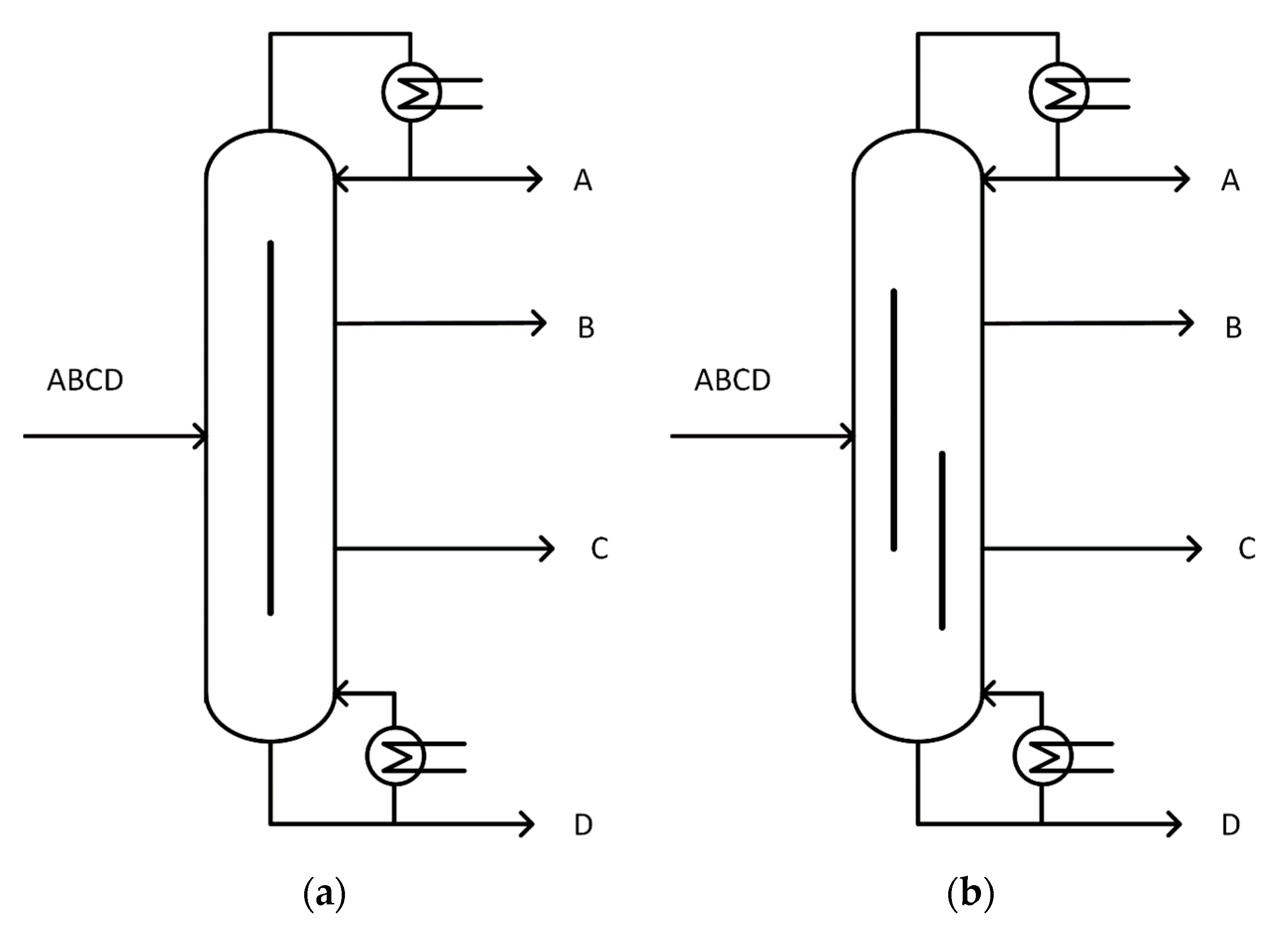
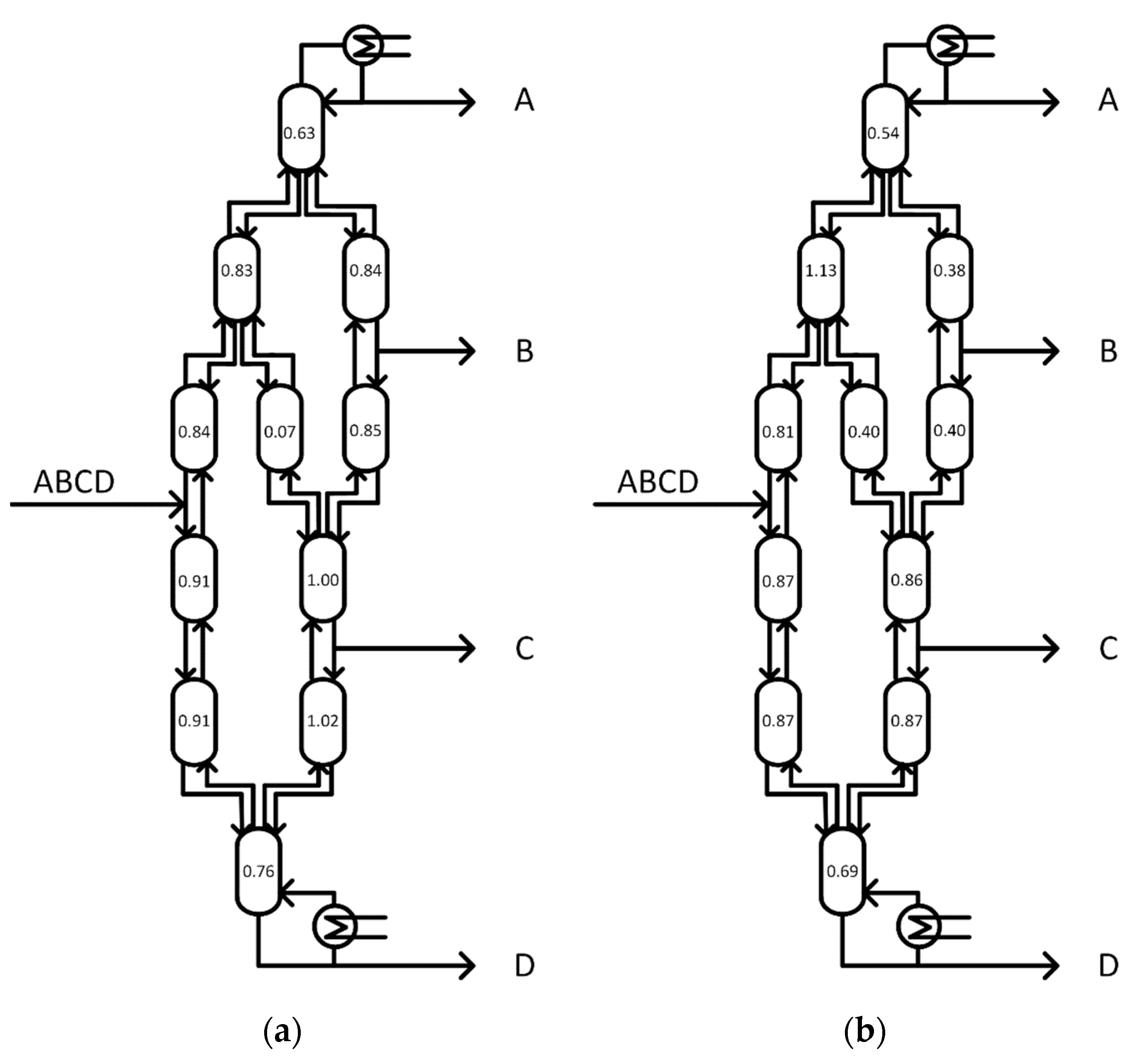
5]. Multiple dividing wall columns (mDWCs) with more than one partitioning wall are the consequent evolution of DWCs, since they offer the possibility to produce four or more pure product fractions in one column shell with further reduction of CAPEX and OPEX compared to classical sequences as the direct split. The mDWC with three partitioning walls (
Figure 1a), also called the 2-3-4 configuration (two products from the prefractionator, three products from the middle fractionator, and four products from the main fractionator), can be operated in the thermodynamic optimum [
6]. This means that it has the minimum energy requirement for the given separation task, as, in every separation section of the column, the easiest separation is always carried out. However, the complexity of this mDWC is increasing compared to DWCs with just one partitioning wall as the degrees of freedom are increasing from 12 to 23 [
7]. This is the reason there is no evidence of a real mDWC plant in operation yet, at neither industrial nor laboratory scale. One opportunity to make an implementation more possible in the future is given by simplified four-product mDWCs, since they can be designed with fewer than three partitioning walls and are therefore easier to realize and operate.
Figure 1b shows a simplification of a mDWC with the second wall in the upper part of the column, referred as the 2-2-4-a configuration. This simplification was already investigated by different authors, since it can be operated with the same energy demand as the 2-3-4 configuration for some specific mixtures of industrial relevance [
8,
9,
10].
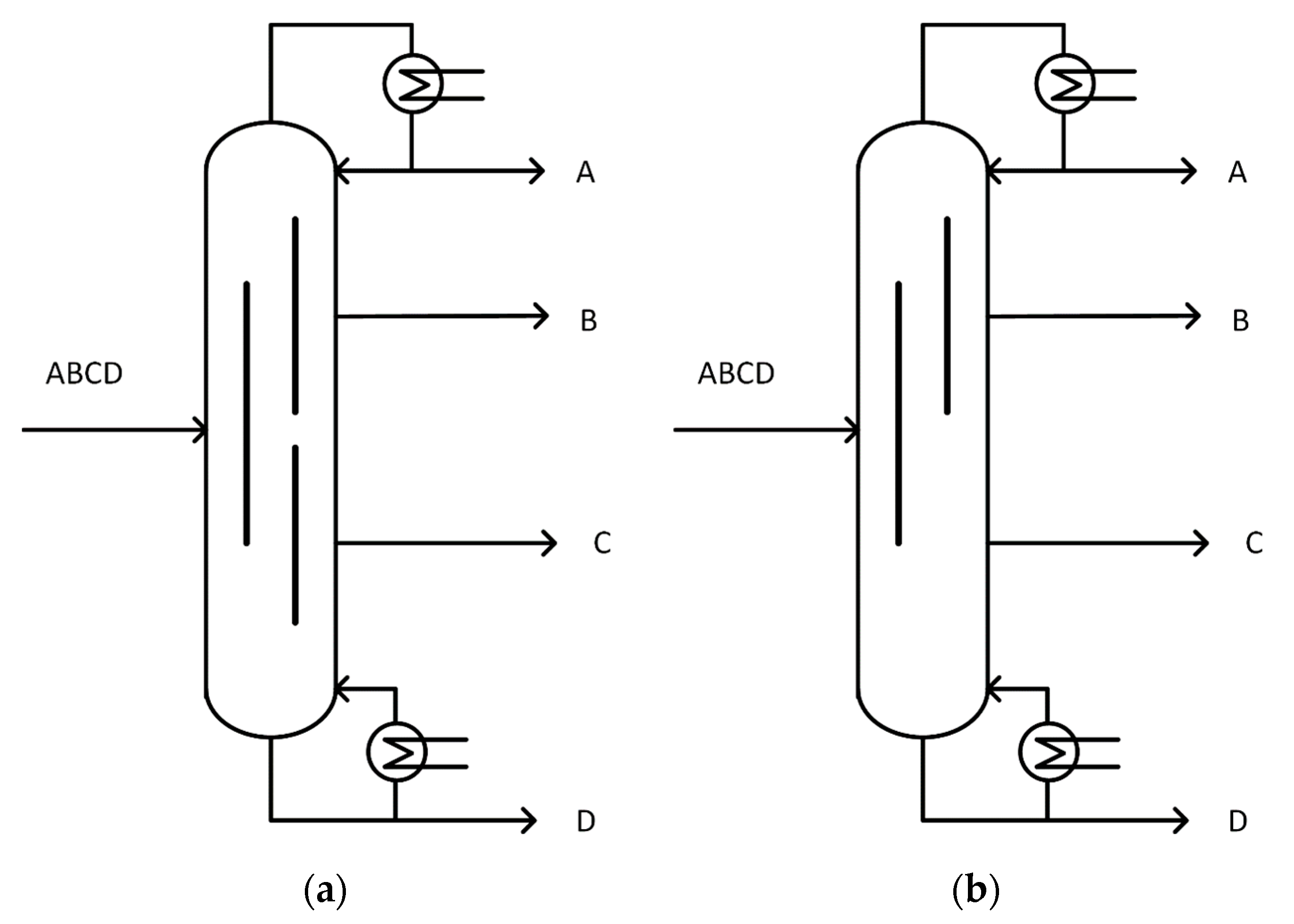
Figure 2 shows other simplified versions of four-product DWCs.
Figure 2a represents the Kaibel Column, a single-partitioned DWC with four product streams [
11]. This column has the big advantage of a relatively simple constructional design, but it cannot be operated in the thermodynamic optimum. In
Figure 2b, another simplified mDWC, which is very similar to the one in
Figure 1b, with the second partitioning wall in the lower area, referred as the 2-2-4-b configuration, is depicted. Whether the 2-2-4-a configuration or the 2-2-4-b configuration is the better choice for a separation task is solely related to the properties of the feed mixture, since the constructional design effort is similar. The big advantage of simplified mDWCs is the reduction of design variables. This is due to the reduced number of partitioning walls, resulting in a reduced number of gas and liquid splits. Different research groups already investigated the potential of an industrial implementation of the 2-2-4-a configuration. A detailed dimensioning of a simplified mDWC with three partitioning walls and two overhead condensers was done by Dejanović et al. In addition, this publication compares five different column configurations of standard DWC and mDWCs, with 2-2-4-a configuration being the best solution [
9]. In another work, Olujić et al. presented an approach of a detailed dimensioning of three different four-product columns. Their investigations on the Kaibel Column, the 2-3-4 configuration and the 2-2-4-a configuration show that the latter is the most suitable for a practical implementation [
10].
For the operational performance of mDWCs, especially the internal gas and liquid splits are crucial. While it is possible to adjust the liquid split by using specifically designed liquid distributors, there is still no way to manipulate the gas split. A recent publication [
12] proposes the application of special chimney trays for the direct manipulation of the vapor split. However, the industrial proof of feasibility for this type of equipment is still missing. Nevertheless, columns with two internal gas splits could not be investigated in practice yet. Therefore, it is difficult to make a prediction about the operational stability of such a column. Remedy can be provided by dynamic simulations, as they can be used for the investigation of control structures or the prediction of the dynamic behavior of the column. Lukač et al. presented two different promising control structures for the 2-2-4-a configuration. For controlling the column, mainly temperature measurements are being used. Their results show that using a temperature difference control for one product stream can respond well to fluctuations in the feed stream composition [
13]. Building a simplified mDWC offers the opportunity of answering questions in regards of the controllability, the behavior of two vapor splits in one column shell and the operation of a column with more than one partitioning wall in general.
This publication presents a structured way from the first idea to the design of the pilot plant in detail. Topics that are discussed in the following parts are the initialization of the simulation, the simulation model and how a promising operating point can be found, the thermodynamic and the fluid dynamic design as well as the sizing of the column.
2. Test Systems and Simulation Model
First, the question must be clarified if the 2-2-4-a configuration or the 2-2-4-b configuration is better suited for a pilot plant realization. Since the applicability of the two setups is determined mainly by the properties of the mixture, the first step was to define potential test systems for the column. Note that the column will be operated in a university environment. Therefore, there are strict constraints regarding toxicity, environmental impact, and fire hazard, as well as the price. For this purpose, a pool of components consisting of six different groups of substances was used to do a feasibility analysis with the main evaluation criteria toxicity, fire hazard and environmental compatibility. Further investigations, such as a price comparison of the components were carried out. In the next step, the Vapor–Liquid Equilibria (VLE) were investigated to prove if azeotropic behavior occurs in binary sub-systems. The physical property package of the process simulator AspenPlus
© V10 was used for this purpose. The test systems applied in the column should strictly show zeotropic behavior. In the case that binary azeotropes occur, it is assured that these systems will not be present in the final mixtures. This resulted in seven different systems that can potentially be used in the mDWC. The pool of components and the resulting systems can be found in
Table A1 in
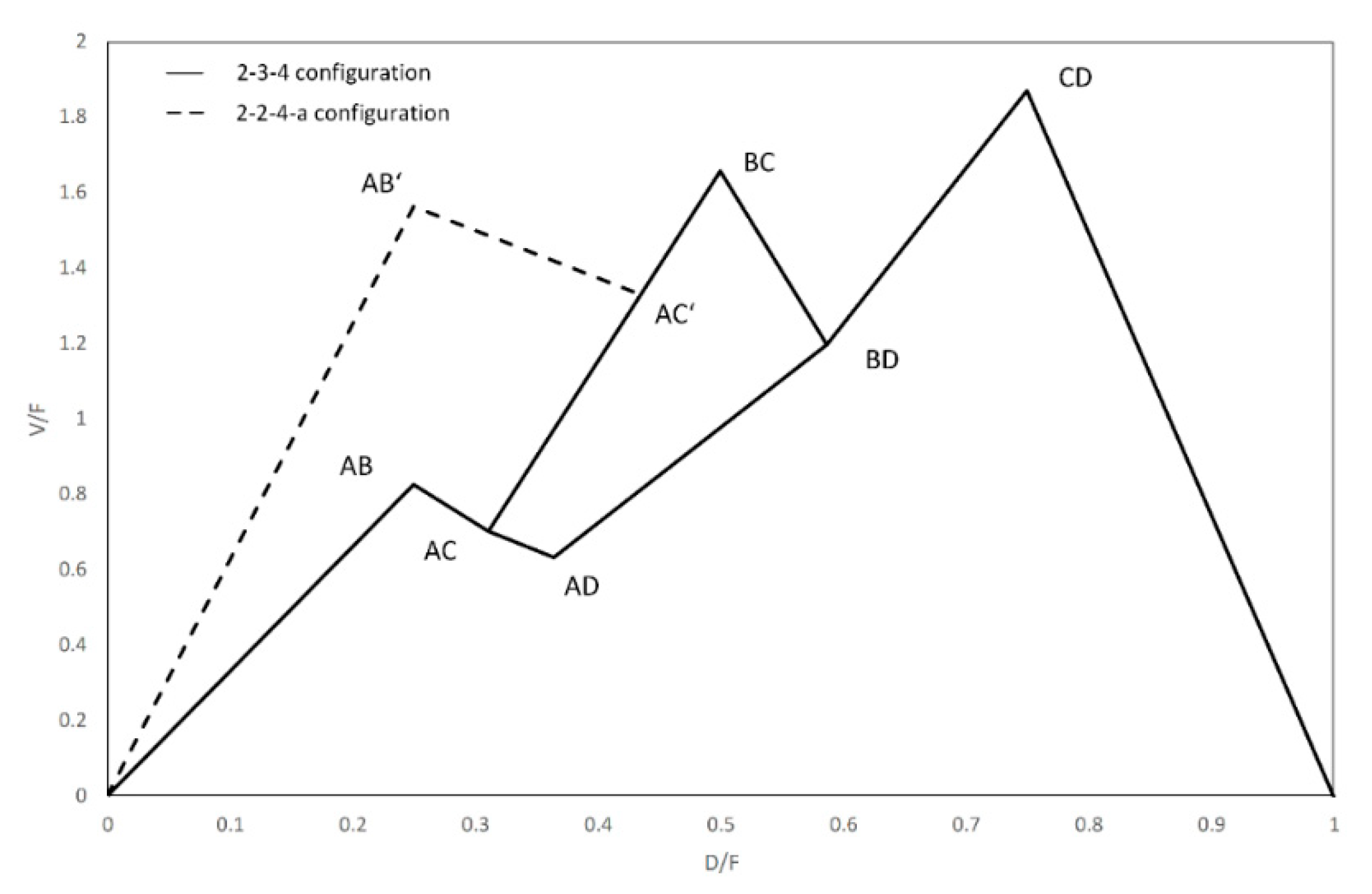
Appendix A. The next step was to check the energy requirement of the two configurations of simplified mDWCs for the chosen mixtures compared to the 2-3-4 configuration, which represents the energetic optimum. This step was carried out based on the
Vmin-diagram. Using
Vmin-diagrams for energetic evaluations is described in detail elsewhere [
7,
14]. Compared to the energetic optimum of the 2-3-4 configuration, all investigated systems within the 2-2-4-b configuration showed a higher energy demand and therefore an energy penalty. For the 2-2-4-a configuration, all investigated systems with the exception of one could be distilled without an energy penalty. This is System 2 in
Table A2 (
Appendix A). A subsequent literature search also proved that the 2-2-4-a configuration is better suited for industrial applications, which is why the decision fell on this configuration [
8,
10,
15].
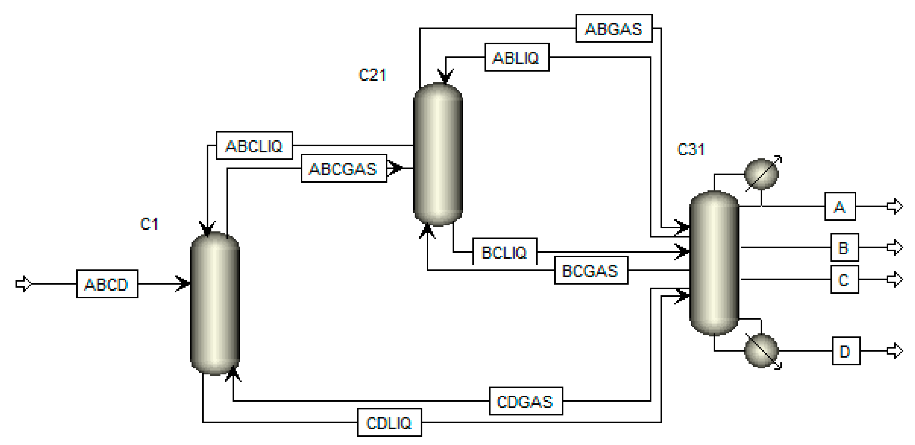
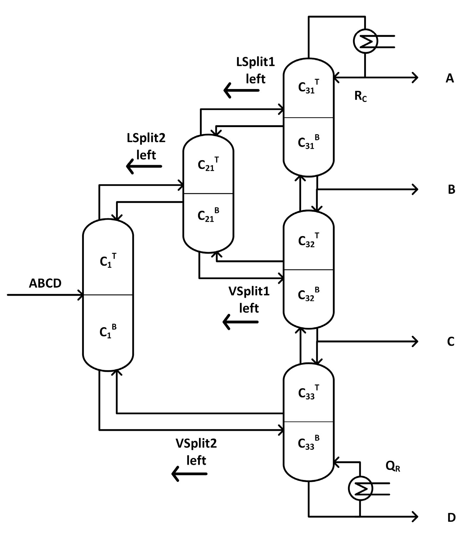
Since commercial process simulators do not offer unit operation models for mDWCs, substitute models have to be applied here [
5]. These are usually built up with thermally coupled simple distillation columns. The most common one is the extended Petlyuk scheme shown in
Figure 3. This is the thermodynamically equivalent substitute model to the mDWC with three dividing walls that shows the minimum energy requirement for any given separation task [
16]. Note that the columns, besides C31 and C33, do not have an evaporator or condenser.
To represent the simplified mDWC configuration, the Petlyuk scheme has to be modified, in a way that the substitute model is thermodynamically equivalent to the 2-2-4-a configuration. The target was to build up the substitute model with the fewest unit operation models and the fewest recycle streams to facilitate the convergence within the simulation.
Figure 4 shows how the resulting model was used in the simulator. To achieve convergence in the initial simulation, meaningful estimations have to be provided for all recycle streams. The estimated values were again found by the
Vmin-method. How simulations are robustly initialized by this method can be found elsewhere [
7,
14]. The thermodynamic model used in the simulation was non-random-two-liquid (NRTL), since it has a very good accuracy and is recommended for alcoholic mixtures, which were solely used in the simulation [
17]. To model the columns within the AspenPlus
© environment, the RadFrac model was used. The equilibrium stage model is absolutely sufficient for the needs of the desired studies. Since the
Vmin-method requests an infinite number of theoretical stages, the initialization of the rigorous substitute model was carried out consequently with an impractically large number of stages. Hence, the stages have to be reduced to a practical number in the next step.
A practical heuristic approach to do this for simple DWCs was presented by Dejanović et al. The proposed approach is described for three-product DWCs. To apply it to four-product mDWCs, some adaptions have to be done. The approach of Dejanović et al. starts the simulation with many stages, i.e. four times the minimum number of stages, calculated by the Fenske equation. Then, the vapor and liquid splits are optimized and the reboiler duty is minimized by using the optimization tool built in ChemCAD
©. This step is repeated, while the number of stages is gradually reduced to a practical number of stages [
18]. To apply this approach to simplified mDWCs, it is important to note that now two gas and liquid splits have to be optimized, while the number of stages is reduced. That means that four different independent variables are used to minimize the objective function (reboiler duty), while the number of stages in each section of the column are gradually and manually reduced. In this work, the optimization tool provided by AspenPlus
© was used.
The determination of the operating point is illustrated by an example. For this purpose, the procedure of Dejanović et al. was used and the necessary adjustments were made to transfer this procedure to four-product mDWCs. The properties of the feed stream used in this example are shown in
Table 1. To ensure that the thermodynamic model was appropriate and thus the simulation results were correct, all binary VLE were first checked using literature data from the Dortmunder Datenbank (DDB). Four components resulted in six binary VLE that have to be checked. The VLE representation of NRTL was in good accordance with the literature data and could be used without further adaptions.
To create the
Vmin-diagram, the relative volatilities were necessary. These were obtained by reading out the K-values from Aspen HYSYS
© V10 and dividing them by the K-value of the heavy boiler, resulting in
. Aspen HYSYS
© was used here, because in contrast to AspenPlus
© this simulator allows reading out the K-values directly from the feed stream. The resulting
Vmin-Diagrams for the 2-3-4 configuration and 2-2-4-a configuration are shown in
Figure 5. Note that there was no energy penalty for this system, since the CD split remained the highest point in the diagram. From this diagram, the necessary information for the initialization of the above-mentioned substitute model was obtained.
To start the simulation, many theoretical stages were provided to approximate an infinite number of stages, as assumed by the
Vmin-method. Fifty stages per separation section were chosen here. The initial values to start-up the simulation are shown in
Table 2. The parameter Quality A, for example, represents the purity of Component A in the stream in which this component occurs most. In the case of Component A, this is the distillate stream. The same applies for the other product qualities in this table. For clarification, the parameters in
Table 2 are referenced in
Figure 6. Note that the section C
1B possessed twice the theoretical stages as all other sections. The reason is explained in
Section 3. The empty lines in the initial value column of
Table 2 are the results of the converged simulation and no values were necessary for the initialization of the simulation.
The results obtained after converged initialization are also shown in
Table 2. Since the product purity after initialization was very poor, it should be mentioned at this point that the
Vmin-method was based on assumptions, such as constant internal molar flows and an infinite number of stages, which no longer held in the presented simulation. Based on this convergent simulation, the AspenPlus
© optimization tool was used to obtain an optimized operating point that meets all given boundary conditions. The boundary conditions were product purities of at least 98 mol-% of the major component in the respective stream. To achieve this, the internal gas and liquid splits were used as independent variables, while the objective function, the reboiler duty, was minimized. Because optimizers generally have problems solving too many different variables, it might be possible to obtain a solution of a local minimum instead of the global minimum. This is due to poorly chosen starting values. To avoid this problem, different starting points were used within the optimization. The best value was then taken as the result. The operating point after applying the optimization for 50 stages in every section is show in
Table 2. Now, all product specifications could be fulfilled, but as expected the reboiler duty increased from 1.98 kW to 2.28 kW. In other words, the minimum energy demand of the
Vmin-diagram cannot be achieved in real operation. Since a practical number of stages is mandatory, the energy demand inevitable increases.
The next step was to reduce the number of stages in all sections and repeat the procedure with the optimization tool. Since the same packings with the same height were installed in all sections, the number of stages in all sections was uniformly reduced. This was conducive to the purpose of keeping the pressure loss equal on both sides of the partitioning walls, which is further discussed in
Section 3. The results of the stepwise minimization of the number of stages are shown in
Table 3. It can be seen that the reboiler duty increased with decreasing number of stages. This result is expected, since more energy is necessary to separate the four components with a lower number of stages.
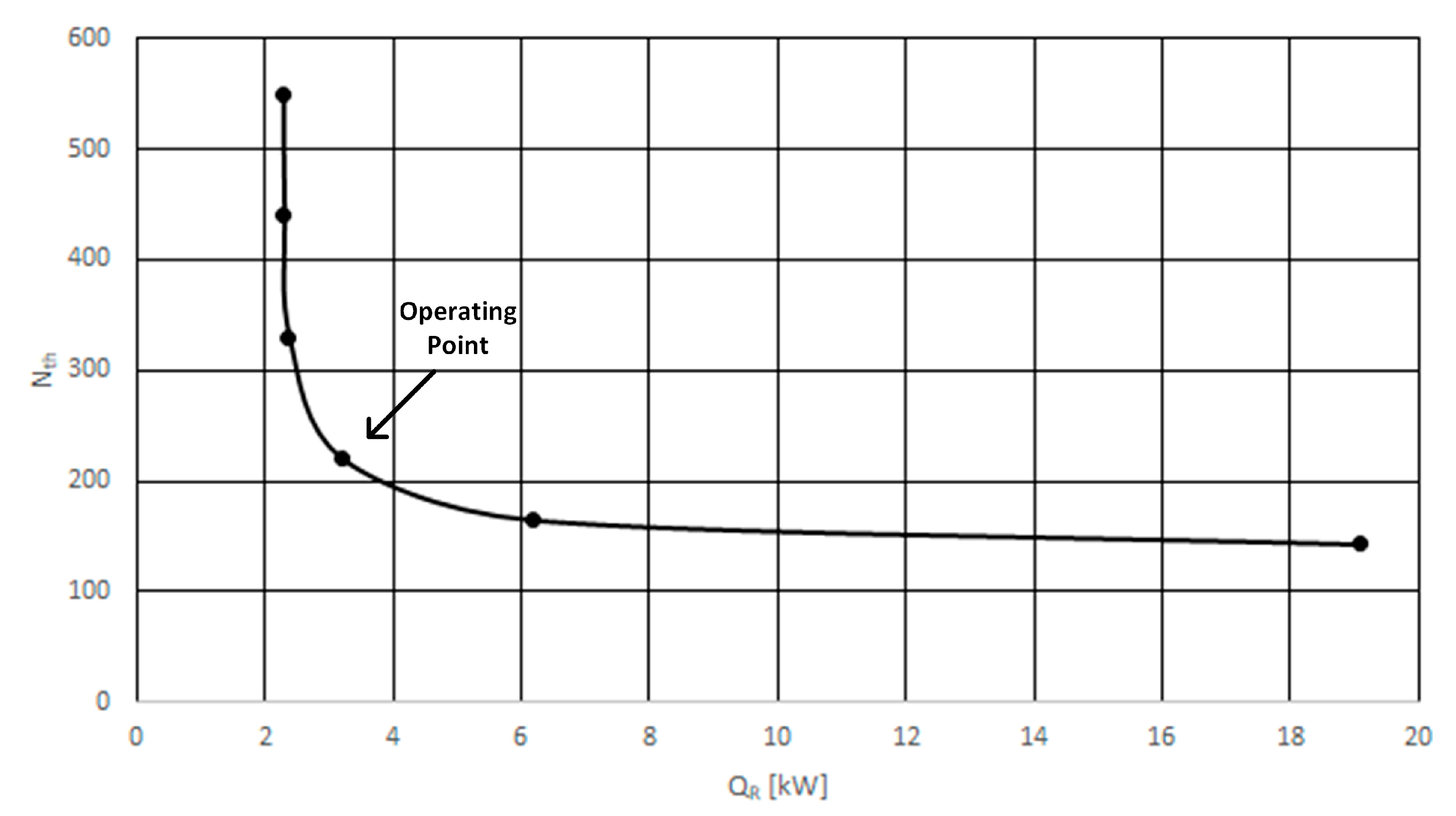
The results in
Table 3 can be understood as a NQ-curve for the 2-2-4-a configuration of a mDWC. Note that a NQ-curve is only valid for one specific product purity for the case that all design parameters are optimized. As shown in
Table 3, the results for the product quality vary in a small range due to the chosen optimization procedure. Strictly speaking, the operating points in
Table 3 are not located on the same NQ-curve. Rather, the points listed there are overlaps of different NQ-curves resulting from the varying product composition. Nevertheless, connecting all points by interpolating the progression in between resulted in the typical shape of a NQ-curve. The NQ-curve shown in
Figure 7 represents the NQ-curve for the product quality of component C being 98 mol%. Included in this diagram are the extreme compromises between the number of stages and the energy demand, represented by the value for the minimum reboiler duty, shown as the highest point in the diagram and the value for the minimum number of stages, shown as the lowest point in the diagram. The number of stages for these two points are 50 stages per section (overall stage number: 550) and 13 stages per section (overall stage number: 143), respectively. The operating point was determined in the area of the greatest curvature, since this is the best compromise between the number of stages and the reboiler duty. This is the final design point of the column.
3. Design of the Pilot Plant
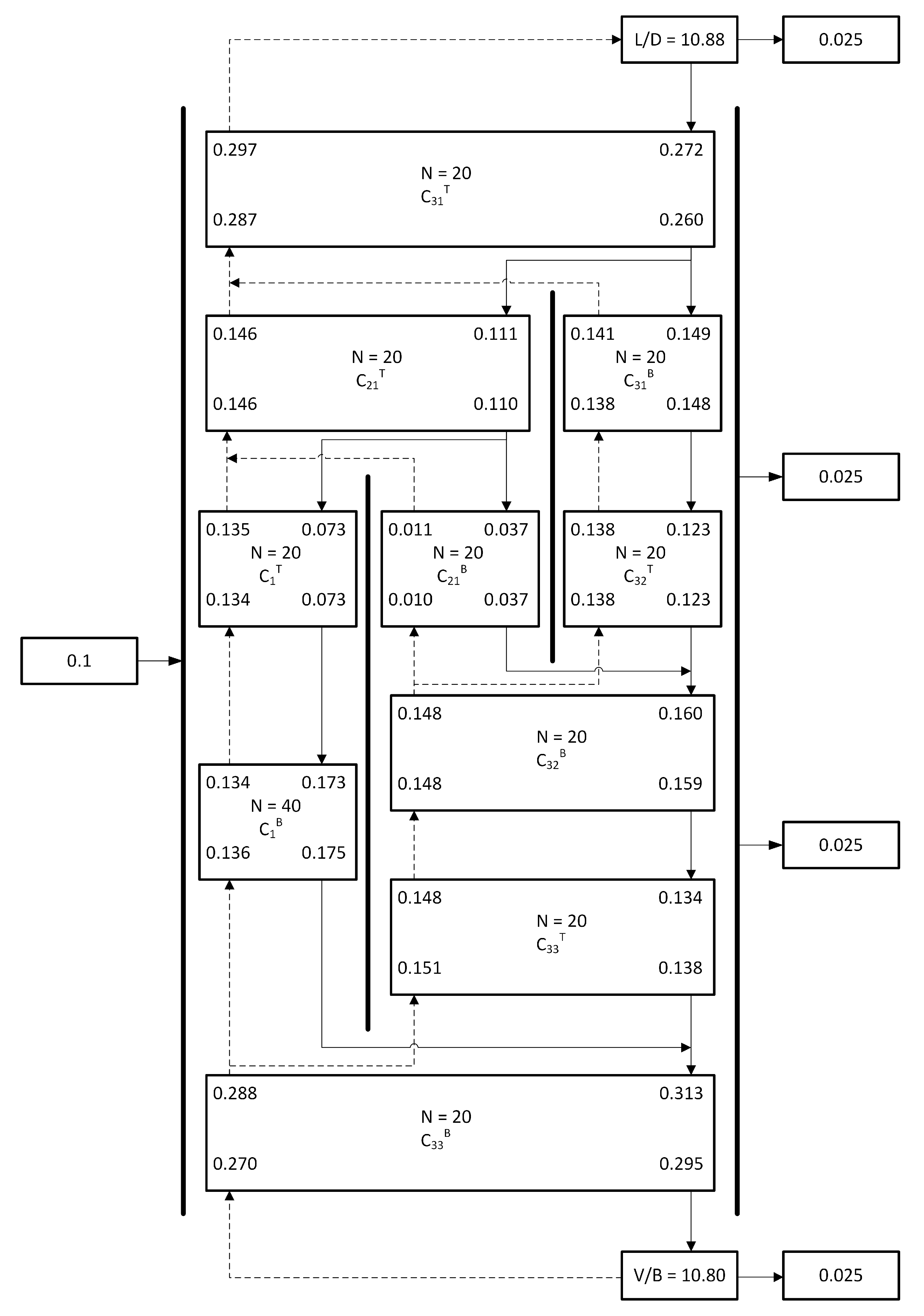
The thermodynamic design from mDWCs (leading to the number of stages and, hence, the internal streams for that specific case) is typically separated from the fluid dynamic design (leading to the areas of the column sections). First, the thermodynamic design is carried out, since it contains the information about the number of stages, as well as the gas and liquid loads in each section. Subsequently, the fluid dynamic design is performed. The thermodynamic design of the column has already been done with the selection of the operating point (see
Section 2).
Figure 8 shows the internal gas and liquid flows at the top and bottom of each section for the chosen operating point and the feed stream shown in
Table 1. In addition, the reflux ratio (denoted as L/D) and the boil up ratio (denoted as V/B), as well as the number of stages in each section are illustrated. Since the feed stream and the side streams are liquid streams, they only influence the liquid load in the column.
Within the fluid dynamic design, the area of each section of the columns has to be determined to realize meaningful loads of vapor and liquid. For this purpose, the internal gas flows obtained from the thermodynamic design are used. The
F-Factor was used as a decision criterion to choose the correct diameters, as it is easy to calculate.
For laboratory packings, usually the
F-Factor should be less than 1. To keep the column flexible, it was decided to go for rather larger diameters for the column sections. This also has positive effects on the heat loss and provides flexibility for future, unknown, separation tasks. Since the mDWC will be realized in a Brugma configuration where all column sections are single shells, a circular cross sectional area can be assumed. The features of the column are further discussed in
Section 4. The chosen diameters is shown in
Table 4. The starting point of our deliberations was to use only a small number of different diameters. This was again to maintain the high degree of flexibility of the plant. The associated
F-Factors are shown in
Figure 9a. It reveals a very small
F-Factor in the column section C
21B, while all other sections can load well. However, these are the
F-Factors obtained from the gas loads of the operating point as determined from the thermodynamic design. From the selection of the section diameters, it becomes clear that the sides of the partitioning walls will have equal cross sectional areas. Moreover, the sections are packed with the same structured packings of the same height. Hence, the pressure loss of the sections is equal and the gas will uniformly split in a 1 to 1 ratio. As a result, the vapor distribution is forced to change due to constructive constraints and can neither be manipulated nor maintained at the original design values. In the next step, the achieved operating point was adjusted, taking the resulting vapor split into account.
Starting from the design case, the vapor splits were adjusted until the same average
F-Factors on both sides of the partitioning walls were achieved to make sure that the gas distributes evenly. Note that an additional section was needed in the area C
1B to keep the pressure drop on both sides of the partitioning walls equal. In this particular case, this meant 60 theoretical stages on the left side of the partitioning wall (C
1T and C
1B) and 60 stages on the right side (20 in C
21B, 20 in C
32B and 20 in C
33T). To find the real gas distribution, the procedure was as follows. First, VSplit2 was set to have an equal
F-Factor on both sides of the partitioning walls. Afterwards, VSplit1 was adjusted, since it depended on VSplit2. When the equal
F-Factors on both sides of the partitioning walls were set, the optimization tool was used to optimize the liquid splits, while reducing the objective function, the reboiler duty. To ensure that the gas was still distributed evenly, this procedure must be repeated until the minimum reboiler duty was found, while all constraints were still fulfilled. The starting
F-Factors in each section for this procedure are shown in
Figure 9a, while the final
F-Factors in each section are shown in
Figure 9b. The values for the internal splits and the product purities are shown in
Table 5. It is noticeable here that the reboiler duty of the adapted gas distribution was now lower and beneath the original value. This is because another operating point with different product specifications was found. The new operating point caused a lower reboiler duty, because the product purity of Component B increased while Component D decreased and, as the
Vmin-diagram in
Figure 5 shows, it was easier to separate Component B from Component C in this mixture than Component C from Component D. It was thus demonstrated that an operating point with the product specifications of at least 98 mol% in every product stream of the column designed in this contribution can be achieved for the given system. Not shown here, but proved, was also the applicability of the other mentioned test systems in the provided column setup. This results from an investigation of the different
Vmin-diagrams of all mixtures. Since the mixture chosen for designing the column was the most difficult one to separate, it can be assumed that all other mixtures could be separated in the same column with the same utilities.
4. Design Features of the Pilot Plant
To build the pilot plant column, the Brugma configuration was chosen, as it is easy to construct and heat transfer across the partitioning walls is eliminated. In addition, it is a proven setup for DWCs with only one partitioning wall [
19].
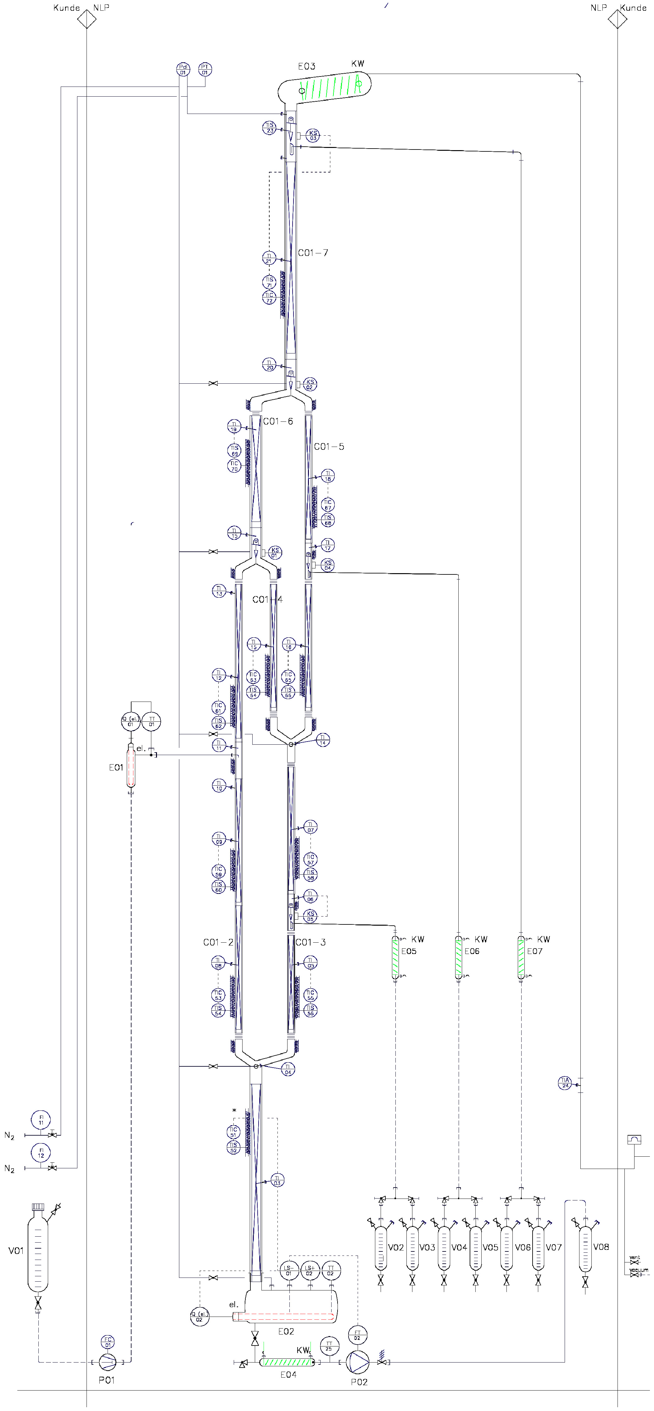
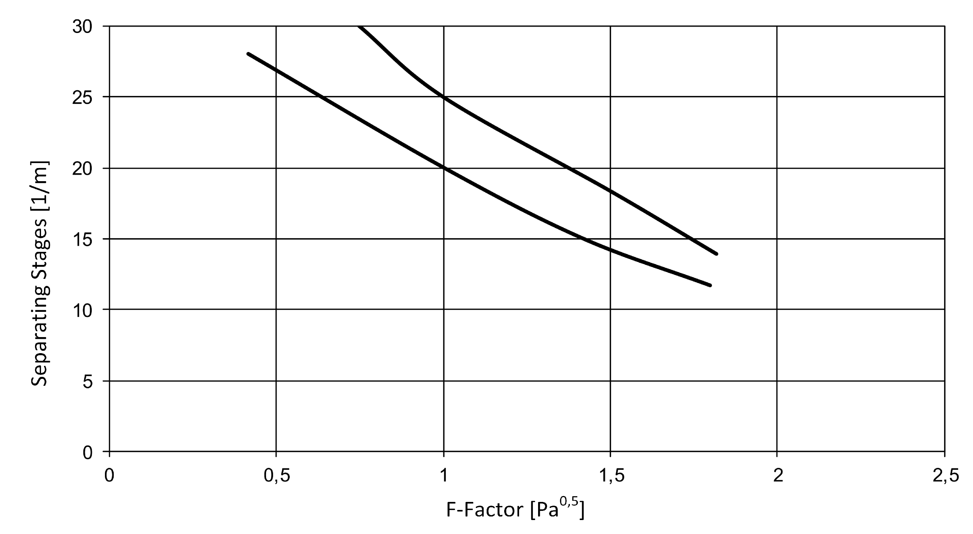
Figure 10 shows the setup of the column. In the Brugma configuration, each separation section is carried out as a separate column and the pilot plant thus does not consist of a single column shell with two partitioning walls but of several thermally coupled simple columns. Since the column should be built in the laboratory facilities of Ulm University, there is a limitation given in the height of the column of 10 m. The height of the column is mainly determined by the number of stages in the main fractionator. The main fractionator consists of sections C
31T, C
31B, C
32T, C
32B, C
33T and C
33B. To accomplish 20 stages per section, it was decided to choose the Montz-Pak A3-1000, since this packing has more than 20 stages per meter at an
F-Factor of less than one (see
Figure A1 in
Appendix B). Each packing is around 1 m long and the main fractionator consists of six different separation sections. Additionally, the two side draws for the product streams as well as the two internal liquid splits are equipped with shaking funnels. Considering the connecting parts for the gas and liquid splits as well as the height of the reboiler and condenser, the pilot plant reaches a height of 9.8 m, thus remaining lower than the limitation of 10 m.
All column shells in this configuration are made of glass. The feed tank is connected via the feed pump, that can be operated with a flow rate of 0–10 L/h, with the prefractionation section of the column. To feed boiling liquid to the column, an electrical feed preheater with a duty of 0.7 kW is installed. The column is equipped with a water cooled condenser in the top and an electric kettle evaporator, providing a duty of 5 kW, in the bottom. In addition, all product streams are cooled by water condensers. First, the column will be operated at atmospheric pressure, with the possibility of implementing a vacuum pump later for the operation in sub-atmospheric pressure. To be able to evacuate the product tanks individually during the operation, they are accomplished redundantly. With the purpose of avoiding heat loss, double-walled, evacuated shells with heating sleeves are used. The column shells are implemented modularly and can easily be exchanged by other column shells with the same height.
To control the column most flexibly, the following control possibilities are available. The distillate flow rate can directly be influenced by the shaking funnel, or can be controlled by a temperature measurement in the section C31T. With the purpose of measuring the temperature profile over the column appropriately and therefore to use these measurements for control issues, PT-100 temperature sensors are installed every 25 cm in the area of the packings. In addition, the side withdrawals as well as the internal liquid distributors can be controlled directly or by a temperature measurement. A pump controls the liquid level of the sump of the column. The evaporator is either controlled by the differential pressure over the entire column or by a temperature measurement in the section C33B. All proposed control possibilities offer a high flexibility as different control structures can be tested in the column. That also ensures that different test systems can be operated with different control structures and thus be separated in the pilot plant properly.


