CFD Simulation and Mitigation with Boiling Liquid Expanding Vapor Explosion (BLEVE) Caused by Jet Fire

Abstract

Different kinds of explosions are driven by the internal energy accumulated in compressed gas or superheated liquid. A well-known example of such an explosion is the burst of a vessel with pressure-liquefied substance, known as Boiling Liquid Expanding Vapor Explosion (BLEVE). Hot BLEVE accident is caused mainly by direct heating (pool fire or jet fire) of the steel casing at the vapor side of the tank to temperatures in excess of 400 °C. Thermal insulation around the tank can significantly reduce and retard the excessive heating of the tank casings in a fire. This will allow fire fighters enough time to reach the accident location and to cool the LPG (Liquid Petroleum Gas) tank to avoid the BLEVE, to extinguish the fire or to evacuate the people in the vicinity of the accident. The proposed algorithm addresses several aspects of the BLEVE accident and its mitigation: Computational Fluid Dynamic (CFD) Simulation of jet fire by using fire dynamics simulator (FDS) software by using large eddy simulation (LES); calculation of the convective and radiative heat fluxes by using the impinging jet fire theory; performing thermochemical and heat transfer analysis on the glass-woven vinyl ester coating of the vessel by using FDS software (version 5); and COMSOL Multiphysics (version 4.3b) during the heating phase of composite and calculation of the time period required to evaporate the liquefied propane by using the first and second laws of thermodynamics.

1. Introduction

Accidental releases of pressure-liquefied materials (by bursts of high-pressure tanks, processing equipment malfunction, etc.) are one of major hazards in process industries, transportation, or storage of flammable materials [1]. Horrific explosions caused by accidental releases of flammable materials into the atmosphere occurred in Port Hudson (USA, 1970), Flixborough (UK, 1974), Mexico City (Mexico, 1984), Ufa (Russia, 1989), Xian (China, 1998), Nechapur (Iran, 2004), Buncefield (UK, 2005) [2]. Different kinds of explosions are driven by the release of internal energy accumulated in compressed gas or superheated, liquid [3]. An example of such an explosion is the burst of a vessel with pressure-liquefied material, known as Boiling Liquid Expanding Vapor Explosion (BLEVE). It is most important physical explosion, i.e., not involving a chemical reaction [4]. 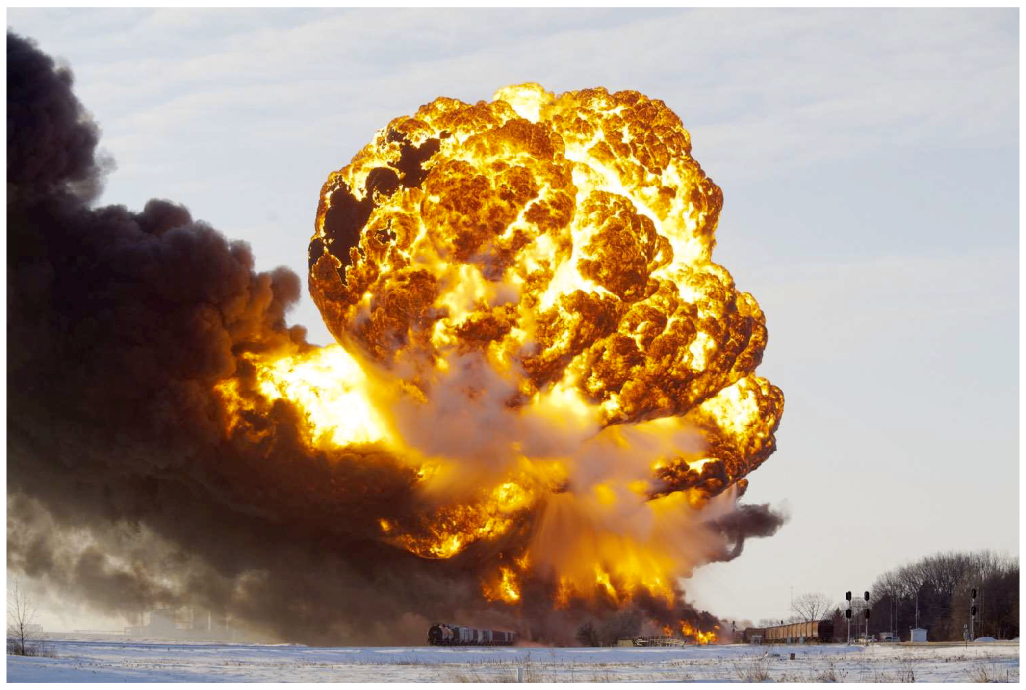It is caused by bursting of a pressurized vessel containing liquid above its atmospheric boiling point [5]. The liquid stored in the vessel may be flammable or non-flammable, such as in a hot water boiler (Steam explosion). If non-flammable, the hazard will be primarily an overpressure event with possible vessel fragmentation. If a flammable material is ignited, it will usually produce a fireball; a secondary effect will be a pressure wave due to the explosively rapid vaporization of the liquid. A photo of BLEVE caused after train derailment in Casselton, North Dakota (2013) is shown in Figure 1 [6].

The earliest observations of detonation waves in gases were made by Berthelot & Vielle [7] and Mallard & La Chatelier [8]. While studying the propagation of flames in tubes they found that under certain conditions combustible gas mixtures propagate flames in tubes with speeds far greater than had been measured previously. The propagation reaches enormous velocities, from 1000 to 3500 m/s, depending on the gas mixture, or many times the velocity of sound at ordinary temperatures and pressures [9]. Detonation waves are sustained by the exothermic chemical reaction that is initiated by the shock compression. They develop from flames in tubes by coalescence of flame-generated pressure pulses into shock waves. Their rate of propagation is limited by the rate at which a shock can travel, and hence it has been possible to develop the theory of propagation based on hydrodynamics alone such extent that detonation velocities may be computed from the physical properties of the explosive medium. There are, however, other aspects of detonation phenomena which are only partially related to hydrodynamic processes and thus are out-side the scope of classical theory. These comprise transition from flame to detonation (DDT—Deflagration to Detonation Transformation), limits of detonation, pulsation, and spin of detonation waves. In addition, various problems arise from observations on the ignition of explosives by weak shocks, and from other incidental observations [9]. A lot of works have been written about mathematical modeling of gas detonations and BLEVE. With the dramatic improvements of computing power, computational fluid dynamics (CFD) modeling has become an increasingly important platform for reformer modeling and design, combining physical and chemical models with detailed representation of the reformer geometry. When compared with first-principles modeling, CFD is a modeling technique with powerful visualization and computational capabilities to deal with various geometry characteristics, transport equations and boundary conditions.

Volpiani et al. [10] has carried out a Large Eddy Simulations (LES) of deflagrating flames by using a dynamic flame wrinkling factor model. His model was validated from a posteriori analysis. Its model can capture both laminar and turbulent flame regimes. At early stages of the flame development, a laminar flame propagates in a flow essentially at rest, corresponding to a unity-wrinkling factor. Transition to turbulence occurs when the flame interacts with the flow motions generated by thermal expansion and obstacles. They have analyzed three distinct configurations:

(1)

The first configuration presents the larger number of obstacles. The interaction between the flame and obstacles created stronger overpressure.

(2)

The second configuration presents the second highest pressure and is characterized by a long laminar phase, once obstacles are placed far away of the ignition point.

(3)

The third configuration, after the flame crossed the first baffle, the flame front is relaminarized before reaching the central obstacle leading to the lowest observed overpressure [10].

Chemical hydrogen hazards are principally associated with the deflagration and detonation phenomena that can be produced when a flammable or explosive mixture of hydrogen and an oxidant is ignited. The minimum energy for the ignition of gaseous hydrogen in air at atmospheric pressure is only 0.02 mJ [11]. Diéguez et al. [11] showed examples of application of CFD to safety issues such as hydrogen leakages, hydrogen flames, detonation, and application of the simulation results to evaluate possible physiological injuries. They performed a CFD for simulating the hydrogen leakage.

Pinhasi et al. [12] applied a numerical-solution method based on the method of characteristics for the investigation of the BLEVE problem. The described method is applied for the solution of the governing equations for unsteady one-dimensional of two-phase flow as well as for the airflow. This method was also employed to calculate the fluid particle path and properties passing the shock wave. For this purpose, a special numerical scheme was derived. The procedure is applied for the numerical integration of the characteristic and compatibility equations, using an explicit numerical scheme.

Scholz & Wuersig [13] have performed CFD calculations of the response of a Moss containment system (Liquified Natural Gas carrier) to pool fire exposure to simulate the transient heating up of the different components. These tanks are insulated with 220 mm polystyrene foam to prevent the heating of tank casings and the boiling of the liquefied natural gas (LNG) in case of exposure to external heating such as pool or jet fires. These tanks are supported by a metal skirt, which transmits the weight of the tank and the cargo to the lower hull.Three physical effects of the heat transfer have been simulated during exposure to pool fire. Inside the solid components of the tank system thermal conduction has been considered. A 2D model has been developed for the analysis of the response of the spherical tank system under pool fire exposure. The scope of the investigation was to calculate the heat flux into the Moss tank system. Melting of the insulation was also considered in their evaluations. The insulation material is also combustible, and in the case of a fire exposure the thermal pyrolysis and degradation of the insulation would be much greater than melting of the insulation. They applied ANSYS software (Version 6.5-1).

The structure of this paper is as follows: In Section 1.1, the measures to avoid hot BLEVE are discussed. In Section 1.2, the computational model is presented briefly. The fire dynamics simulator (FDS) software is described in detail in Section 2.1 and Section 2.2. Section 2.3 describes the calculation method of the jet fire impinging heat flux. Section 2.4 describes the heat transfer and thermochemical analyses on the composite coating of the tank. The thermodynamic analysis of the propane is described in Section 2.5. Section 3 presents the FDS models and COMSOL (version 4.3b) results. The described work contains new tools and methods. The CFD simulation of the heptane impinging jet was carried by using the FDS (version 5). The previous works which have been written about thermal protection of BLEVE accident, have assumed that the external surface of lining is fixed (i.e., there is not recession of the lining). This work contains the modeling of the recession phenomena. It should be noted that numerical modeling of thermochemical erosion is still complicated issue. The numerical modeling requires much more knowledge than the conventional heat transfer approach such as: Arrhenius coefficients (the data is obtained from experiments), and enthalpy of formation virgin material (the data is obtained from calorimeter experiments). The coupling of the FDS results with COMSOL can extend the capabilities of the algorithm and to address other issues concerned with BLEVE accident such as: transient heating of the steel, structural analysis of the lining and steel tank as a function. The structural analysis of the steel casing is essential to verify that the structural integrity of the tank under the BLEVE accident. The proposed algorithm is very flexible. It is possible to perform simulation of methane or other Hydrocarbon fuels jet fires. Other insulations (rubber, PMMA etc.) can be tested. It is probably the first time that FDS software has been applied to simulate jet fire impinging on composite lining and causing thermochemical ablation on the tank lining.

1.1. Measures to Avoid Hot BLEVE

Hot BLEVE is caused mainly by heating of the steel casing at the vapor side of the tank to temperatures in excess of 400 °C. Thermal coating around the tank can considerably attenuate the excessive heating of the tank casing in case of exposure to fire. This will allow fire fighters enough time to reach the accident location and to cool the LPG (Liquid Petroleum Gas) tank to prevent the BLEVE, to extinguish the fire or to evacuate the people in the vicinity of the tank. Important is that the insulation (coating) attenuates the heating of the tank casing long enough [14]. At present, there are three different types of coatings [15]:

• Intumescent fire protection coatings are based on epoxy resin. When they are exposed to fire, at temperature of around 150–200 °C, they react independently by forming foamed protective insulating layer. The foamed coating forms a thermal barrier layer, which reduces the heat flux input to the tank walls. Most of these coatings contain three main ingredients: An acid source, a carbon source, and a blowing agent. The formulation of the coating must be optimized in terms of physical and chemical properties to form an effective protective char layer [16,17,18].
• Sublimation fire protection coatings release gases under thermal loads. In the case of exposure to fire, large quantities of thermal energy are needed to transform the coating directly from the solid to the gaseous aggregate state without liquefying beforehand (phase transformation). This transformation is used to build up a layer which absorbs and reduces the heat flow into the tank walls.
• Ablative coatings are based on endothermic processes. The heat transfer is delayed by the extraction of chemically bonded water from the fire protection coating.

In this work a thermochemical ablation model has been developed and carried out on glass-woven vinyl ester coating. Glass Fiber Reinforced Plastic (GFRP) is an advanced innovation for the transportation of flammable materials. Its light weight reduces the transportation costs [19]. A key limitation of composite materials is their rapid loss of structural stability in fire. At temperatures between 100 °C and 200 °C, the matrices consisting of thermosetting polymers such as epoxy or polyester resin start to soften and weaken. This leads to a decrease in the structural integrity of the composite material [20].

1.2. Algorithm Description, Assumptions and Scope

In this work, it is assumed that heptane jet fire is impinging on the external boundary of the tank composite lining. The distance between the jet source and the tank is 3 m. The exposed diameter of the lining is 0.8 m. The lining is made of glass-woven vinyl ester. It is assumed that the thickness of lining is 0.02 m (20 mm). The cylindrical tank casing is made of steel AISI 310. This steel type has higher ultimate tensile strength. It has also excellent high temperature properties with good ductility and weldability. It is designed for high temperature service. It resists oxidation in continuous service at temperatures up to 1150 °C and has good Corrosion resistance. The tank initially contains liquid propane. The initial temperature of the propane inside the tank is 55.6 °C. The initial pressure inside the tank is 1930 kPa. The thickness of the steel tube is 12.2 mm (w). The internal diameter of the tank is 1.2 m (D_i). The tank contains 500 kg of liquefied propane (the vapor quality of the propane is x = 0). The left side of the tank is exposed to jet fire heating. At the liquid side (bottom) of the tank the heat of the fire will be transferred via the steel casing wall to the liquid and cause evaporation of the liquid propane (see Figure 2).

As the liquid propane evaporates completely (vapor quality is x = 1) the temperature and vapor pressure will be increased (for propane 19 bar at 55.6 °C). At the phase of superheated vapor, the pressure of the propane inside the tank will increase with the temperature. However, if the temperature of the steel on the gas side of the tank exceeds 450–550 °C the steel will lose its integrity and the tank will rupture [14]. This will also occur if a tank is equipped with a Pressure Relief Valve (PRV). The set point of the PRV of the tank vehicles is generally set at 1.93 MPa for propane mixtures. The material stress can be calculated with [14]:

$$\sigma =\frac{p_i{D}_i}{2w}$$

(1)

where $\sigma$ is the stress in (MPa), $p_i$ is the internal pressure of the tank in (MPa), $D_i$ is the diameter of the tank and $w$ is the of the tank wall. This results in a material stress of 189 MPa. The propane tank should be able to withstand this pressure. If the material stress exceeds the strength of the tank the tank will fail. In Figure 3 the strengths of several steels are shown as a function of temperature [21]. The material stress exerted on the by the pressurized propane is shown for comparison.

Figure 3 shows that the Ultimate Tensile Strength of the Stainless Steels decreases with the temperature. The AISI 310 has the maximal tensile strength.

In this work a CFD simulation and mitigation study BLEVE has been performed. The proposed computational work is composed of five phases:

(a)

Simulation of jet fire by using FDS software

(b)

Calculation of the convective and radiative heat fluxes by using the impinging jet fire theory

(c)

Heat transfer analysis on the composite coating of the vessel by using FDS software (version 5) and COMSOL Multiphysics (version 4.3b) during the heating phase of composite

(d)

Calculation of the time period required to evaporate the liquefied propane

(e)

Structural analysis on the tank steel casings

It is important to be able to design thermal coatings for gas pipes and storage tanks that can withstand such catastrophic events. Explosive pressure and structural damage can be estimated with analytical and numerical tools. By using the described computational tools, it is possible to postpone or even to prevent this accident. Important issue which should be considered is that the insulation (coating) attenuates the heating of the tank wall long enough.

2. Materials and Methods

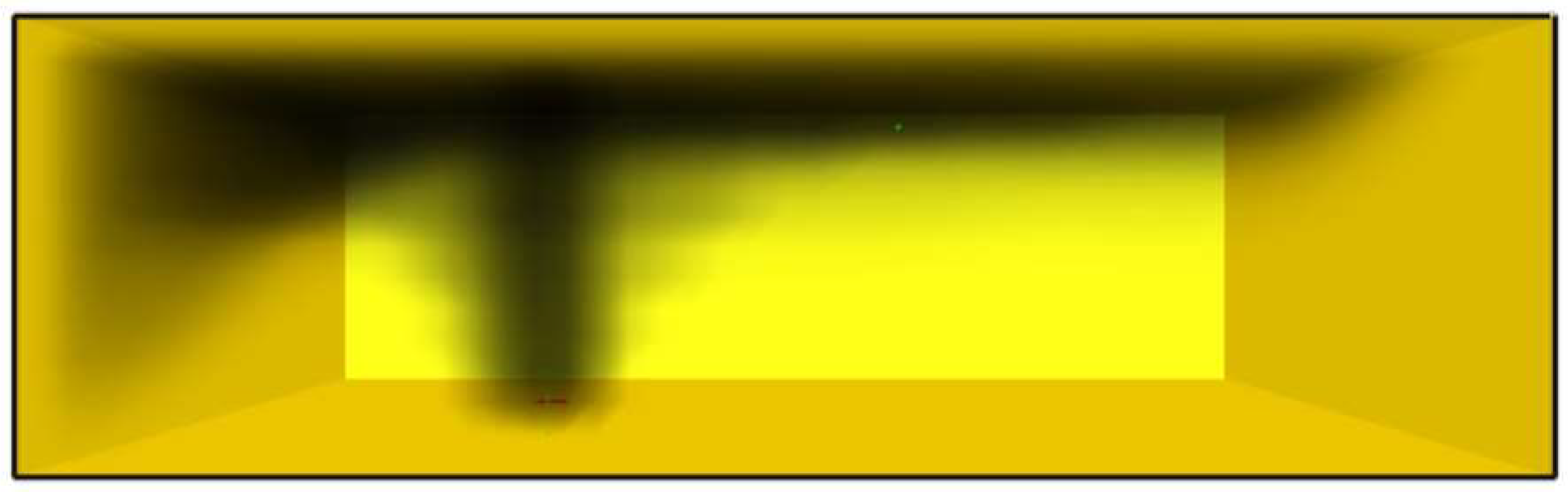
2.1. Fire Dynamic Simulation Modeling of the Jet Fire

In flames formed by fuel jets in the atmosphere the combustion process is coupled with the process of mixing. An analysis of such flames requires consideration of the mixing process only. Flames of fuel jets range from slow combustion exemplified by candle flames where the stream filaments are laminar and mixing occurs by molecular diffusion only to rapid fuel combustion in industrial furnaces and engines of various types, where mixing is accomplished by turbulent eddy motion [9]. In this work CFD study of Jet Flames has been performed by FDS software. The FDS has been developed at the National Institutes of Standards and Technology (NIST), e.g., McGrattan et al. [22,23]. This software calculates simultaneously the velocity, pressure, temperature, density, and chemical composition (mole fraction) within each numerical grid cell at each discrete time step. The FDS software also has a visual post-processing image simulation program named "smoke-view".

This software performs conjugated heat transfer analysis on the solid walls i.e., it solves simultaneously the temperature of the gaseous products and the temperatures at the external surfaces of the solid walls.

It also calculates the temperature, heat flux, and mass loss rate of the enclosed solid surfaces (thermochemical pyrolysis). We shall see later that the mass loss rate is controlled by Arrhenius equations. The latter is used in the case where the fire heat release rate is unknown. The major components of this software are:

Radiation Transport—The FDS software solves the Radiation Transport Equation (RTE) for a non-scattering gray gas. In a limited number of cases, a wide band model can be used in place of the gray gas model. The RTE is solved by using the Finite Volume Method (FVM) [23].

Combustion Model—FDS uses a mixture fraction combustion model. The mixture fraction is a conserved scalar quantity that is defined as the fraction of gas at a given point in the flow field that originated as fuel. This software assumes that combustion is mixing controlled, and that the reaction of fuel and oxygen is infinitely fast. The mass fractions of all the major reactants and products can be derived from the mixture fraction by means of “state relations,” empirical expressions arrived at by a combination of simplified analysis and measurement [24].

Hydrodynamic Model—FDS code is formulated based on CFD of fire-driven fluid flow (Natural convection). The numerical solution can be performed by using either a Direct Numerical Simulation (DNS) method or LES. The latter is relatively low Reynolds numbers and is not severely limited in grid size and time step as the DNS method. This software cannot perform CFD simulations on high Mach number applications.

In addition to the classical conservation equations solved by FDS software (including mass species momentum and energy), it also solves thermodynamics-based state equation for a perfect gas.

2.2. Governing Equations of FDS Software

The following sections introduce the conservation equations for mass, momentum, and energy for a Newtonian fluid.

2.2.1. Mass and Species Transport

Mass conservation is expressed terms of the density, $\rho$ [22]:

$$\frac{\partial \rho }{\partial t}+\nabla \cdot \rho u={{\dot{m}}^{‴}}_b$$

(2)

where $\rho$ denotes the density (kg/m³), and $u$ denotes the velocity field (m/s). This equation is expressed terms of each gaseous species, $Y_{\alpha }$:

$$\frac{\partial }{\partial t}\left(\rho Y_{\alpha }\right)+\nabla \cdot \rho Y_{\alpha }u=\nabla \cdot \rho D_{\alpha }\nabla Y_{\alpha }+{{\dot{m}}^{‴}}_{\alpha }+{{\dot{m}}^{‴}}_{b,\alpha }$$

(3)

$D_{\alpha }$ denotes the diffusion coefficient of $\alpha$ component of the mixture (m²/s).

2.2.2. Momentum Transport

The momentum equation in conservative form is written [22]:

$$\frac{\partial }{\partial t}\left(\rho u\right)+\nabla \cdot \rho uu+\nabla p=\rho g+f_b+\nabla \cdot {\tau }_{ij}$$

(4)

Here $f_b$ denotes the force term (Pa/m). The stress tensor, ${\tau }_{ij}$ (Pa), is defined [22]:

$$\begin{array}{l}{\tau }_{ij}=\mu \left(2S_{ij}-\frac{2}{3}{\delta }_{ij}\left(\nabla \cdot u\right)\right);{\delta }_{ij}=\{\begin{array}{l}1i=j\\ 0i\ne j\end{array};S_{ij}=\frac{1}{2}\left(\frac{\partial u_i}{\partial x_j}+\frac{\partial u_j}{\partial x_i}\right)i,j=1,2,3\end{array}$$

(5)

The term S_ij denotes the symmetric rate-of-strain tensor. The symbol μ denotes the dynamic viscosity of the fluid. In this work the overall computation is carried out by using LES, in which the large-scale eddies are calculated directly, and the subgrid-scale dissipative processes are modeled. The numerical algorithm is designed so that LES becomes DNS as the grid is refined. It should be noted that in most fire simulation applications, FDS uses LES. For example, in simulating the flow of smoke through a large, multi-room enclosure, it is not possible to obtain the combustion and transport processes directly.

2.2.3. LES

One of the most dominant features of any CFD model is its treatment of turbulence. Among the three main techniques of simulating turbulence i.e., Reynolds Averaged Navier Stokes (RANS), LES, and DNS, FDS uses only LES and DNS. LES is a technique used to model the dissipative processes (viscosity, thermal conductivity, material diffusivity) that occur at length scales smaller than those that are explicitly resolved on the numerical grid. This means that these parameters in the equations above cannot be used directly in most practical simulations. They must be replaced by surrogate expressions that “model” their impact on the approximate form of the governing equations. This sub section contains a simple explanation of how these terms are modeled in FDS. There is a small term in the energy equation known as the dissipation rate, $\epsilon$, (Pa/s) the rate at which kinetic energy is converted to thermal energy by viscosity [22]:

$$\begin{array}{l}\epsilon ={\tau }_{ij}\cdot \nabla u=\mu \left(2S_{ij}\cdot S_{ij}-\frac{2}{3}{\left(\nabla \cdot u\right)}^2\right)=\mu [2{\left(\frac{\partial u}{\partial x}\right)}^2+2{\left(\frac{\partial v}{\partial y}\right)}^2+2{\left(\frac{\partial w}{\partial z}\right)}^2+\\ {\left(\frac{\partial v}{\partial x}+\frac{\partial u}{\partial y}\right)}^2+{\left(\frac{\partial w}{\partial y}+\frac{\partial v}{\partial z}\right)}^2+{\left(\frac{\partial u}{\partial z}+\frac{\partial w}{\partial x}\right)}^2-\frac{2}{3}{\left(\frac{\partial u}{\partial x}+\frac{\partial v}{\partial y}+\frac{\partial w}{\partial z}\right)}^2]\end{array}$$

(6)

The viscosity μ is modeled

$${\mu }_{LES}=\rho {\left(C_s\Delta \right)}^2{\left(2{\overline{S}}_{ij}:{\overline{S}}_{ij}-\frac{2}{3}{\left(\nabla \cdot \overline{u}\right)}^2\right)}^{\frac{1}{2}}$$

(7)

where C_s denotes an empirical constant and $\Delta$ is a length on the order of the size of a grid cell. The bar above the various quantities denotes that these are the resolved values, meaning that they are computed from the numerical solution sampled on a coarse grid (relative to DNS). The other diffusive parameters, the thermal conductivity and material diffusivity, are related to the turbulent viscosity by [22]:

$$k_{LES}=\frac{{\mu }_{LES}{c}_p}{P{r}_t};{\left(\rho \mathrm{D}\right)}_{t,LES}=\frac{{\mu }_{LES}}{S{c}_t}$$

(8)

The turbulent Prandtl number $P{r}_t$ (defined as the ratio of momentum diffusivity to thermal diffusivity) and the turbulent Schmidt number $S{c}_t$ (defined as the ratio of momentum diffusivity to mass diffusivity) are assumed to be constant for a given scenario. The model for the viscosity, ${\mu }_{LES}$, serves two roles: first, it provides a stabilizing effect in the numerical algorithm, damping out numerical instabilities as they arise in the flow field, especially where vorticity is generated. Second, it has the appropriate mathematical form to describe the dissipation of kinetic energy from the flow.

2.2.4. Energy Transport

The energy conservation equation is written in terms of the sensible enthalpy, $h_s$ (J/kg) [22]:

$$\frac{\partial }{\partial t}\left(\rho h_s\right)+\nabla \cdot \left(\rho h_{s}u\right)=\frac{Dp}{Dt}+{\dot{q}}^{‴}-{\dot{q}}_b^{‴}-\nabla \cdot {\dot{q}}^{″}+\epsilon$$

(9)

The sensible enthalpy (J/kg) is a function of the temperature [22]:

$$h_s={\displaystyle \sum _{\alpha }{Y}_{\alpha }{h}_{s,\alpha }}$$

(10)

where sensible heat of each component in the mixture is calculated by [22]:

$$h_{s,\alpha }\left(T\right)={\displaystyle \underset{T_0}{\overset{T}{\int }}{c}_{p,\alpha }\left(T^{\prime }\right)d{T}^{\prime }}$$

(11)

here ${\dot{q}}^{‴}$ denotes the volumetric heat release rate produced from a heptane oxidation (W/m³), ${{\dot{q}}^{‴}}_b$ denotes the energy transferred to the evaporating heptane liquid (W/m³) and ${\dot{q}}^{″}$ represents the conductive and radiative heat fluxes (W/m²) [22]:

$${\dot{q}}^{″}=k\nabla T-{\displaystyle \sum _{\alpha }{h}_{s,\alpha }\rho D_{\alpha }\nabla Y_{\alpha }+q_r^{″}}$$

(12)

2.2.5. Equation of State

The pressure is computed by applying the ideal gas equation of state (Frequently the jet fire occurs at atmospheric pressure which is much less than the critical pressure of the gaseous mixture):

$$p=\frac{\rho \overline{R}T}{\overline{W}}$$

(13)

where p denotes the pressure in (Pa), T is the temperature in (K), $\overline{R}$ is the gas constant and $\overline{W}$ is the molar mass of the gaseous mixture in (J/mole).

2.3. Calculation Method of the Jet Fire Impinging Heat Flux

Impinging flame jet has been extensively investigated due to their importance in a wide range of applications [25]. Two heat transfer mechanisms have been considered in this work: forced convection and radiation. The total heat flux was considered in FDS transient thermochemical ablation and conduction calculations [24].

2.3.1. Convective Heat Transfer

Heat is transferred between the jet impingent turbulent flow and the solid surface [26].

2.3.2. Radiative Heat Transfer

In the jet fire, most if the heptane burns in turbulent diffusion flame as fuel and air mix together. The flame is highly luminous, and soot particles are formed during the combustion process [26]. The radiative heat transfer within the heptane jet fire is composed of the thermal radiation from high temperature burned gases and the radiation from soot particles.

2.3.3. Calculation of the Maximal Heat Flux Value

The maximal total heat flux (composed of radiative and convective) is calculated by using the following Equation [25]:

$${q^{″}}_{\max ,conv+rad}=10{\left(q_f\right)}^{0.3}$$

(14)

It is based on a thermal input of $q_f=60-1600\mathrm{kW}$. The values of the thermal input were taken from FDS calculation results.

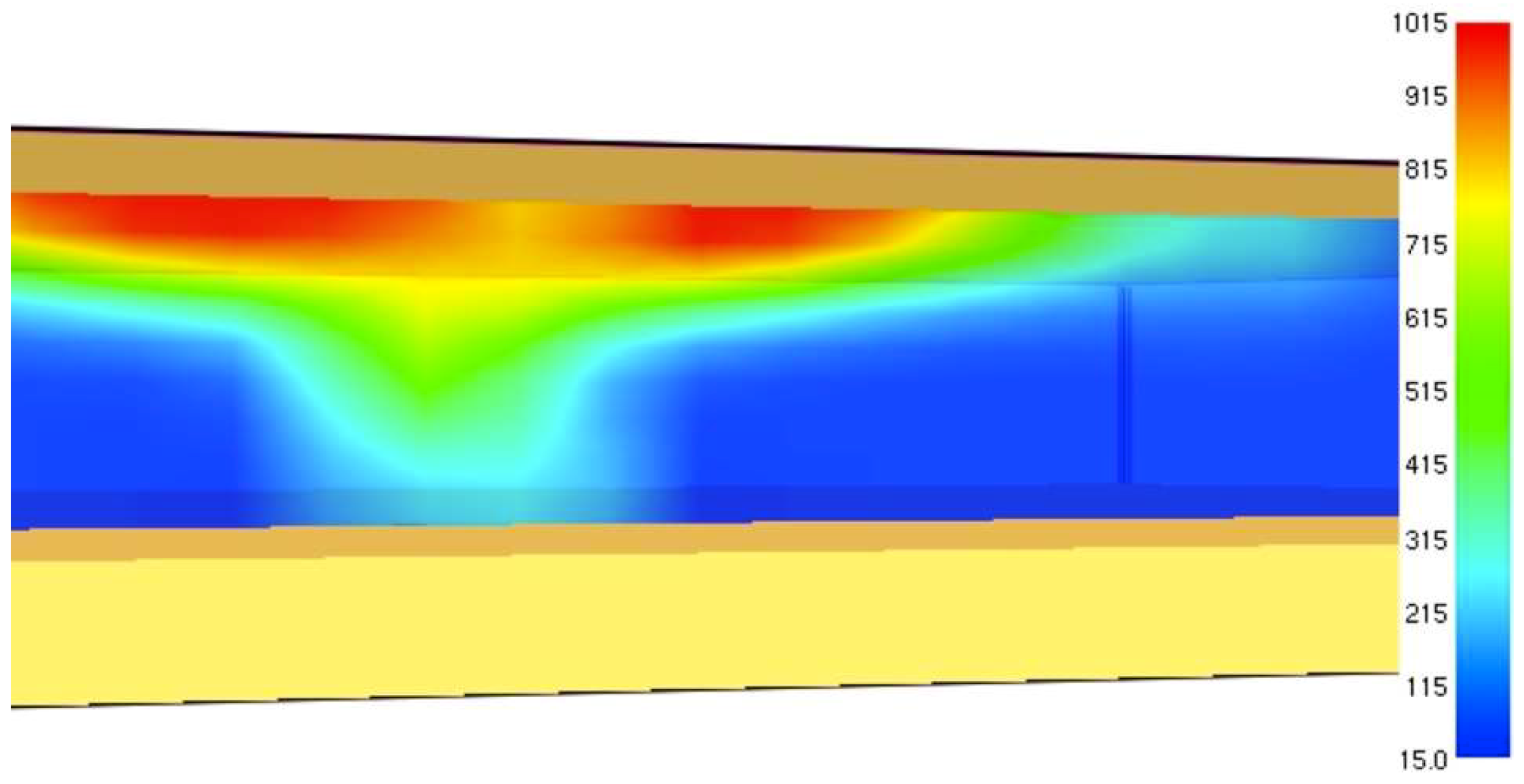
2.4. Heat Transfer and Thermochemical Analyses on the Composite Coating of the Tank

The proposed approach can be divided into two simulation parts.

In first part, the analysis of composite has been carried out under jet fire thermal loads by using the FDS (see Section 2.5). The FDS code is used to solve for the recession of the surfaces as a function of time. The temperature and heat flux of the interior structural surface profiles are used and applied to subsequent simulation part. In the second part, COMSOL heat transfer module (version 4.3b) has been applied to calculate the temperature profiles through the thickness of the composite by importing the instantaneous surface temperatures and the recession obtained from the FDS model. In this work, we have assumed that the composite decomposed to a pyrolysis gas plus char. The reaction scheme is shown [27]:

$$P\to \alpha G+\left(1-\alpha \right)C$$

(15)

During the pyrolysis reaction, mass of the polymer is consumed and produces a fraction, $\alpha$, of gas and the remaining char. The first order reaction rate for the composite is:

$$\frac{d{r}_p}{dt}=-k_0{r}_p$$

(16)

where $r_p$ denotes the instantaneous thickness of the polymer in (m), t is the time in (s) and $k_0$ denotes the rate constant for pyrolysis reaction in (1/s). The rate constant in for the pyrolysis reaction, $k_0$, is a function of temperature and is better described by the Arrhenius relationship [27]:

$$k_0=A_0\cdot \exp \left[-\frac{E_{A0}}{R\cdot T}\right]$$

(17)

where $A_0$ is the pre-exponential factor of pyrolysis reaction (1/s). $E_{A0}$ is the activation energy of pyrolysis reaction (kJ/kmol), R is universal gas constant ((J/mole)/K) and T is the temperature in (K). The pre-exponential factor and activation energy can be found by thermogravimetric analysis. A 1D heat conduction equation for the composite temperature $T_s\left(x,t\right)$ is applied in the direction x pointing into solid (the point x = 0 represents the surface) [22]:

$${\rho }_s{c}_{p,s}\frac{\partial T_s}{\partial t}=\frac{\partial }{\partial x}\left({\lambda }_s\frac{\partial T_s}{\partial t}\right)+{\dot{q}}_s$$

(18)

The source term, ${\dot{q}}_s$, consists of chemical reactions (production or loss) rate given by the pyrolysis models for different types of solid and radiative absorption and emission in depth [22].

$${\dot{q}}_s={\dot{q}}_{s,c}+{\dot{q}}_r$$

(19)

The chemical source term of the heat conduction equation consists of the heat of the reaction [22]:

$${\dot{q}}_{s,c}=-{\rho }_s{k}_0\Delta H_r$$

(20)

$\Delta H_r$ is the heat of reaction. The thermal properties (thermal conductivity, heat capacity and density) and the rate constants of the composite used in the calculation of FDS and COMSOL are shown in

Table 1. Thermophysical and thermochemical properties of E-Glass vinyl ester used in calculations [28].

Material Property	Value
rho	1140 kg/m3
Cp	760 J/(kg·°C)
λ	0.43 w/(m·°C)
E	2.13 × 105 kJ/kmol
A	5.59 × 1013 1/s
n	1
ΔH	378,800 J/kg

[28].

As was stated before the receding surface is exposed to radiative and convective heat flux (see Equation (14)). FDS software calculates the convective heat flux by using the following Equation [22]:

$${\dot{q}}_c=h\left(T_g-T_w\right)$$

(21)

According to the LES approach, the convective heat flux to the surface is calculated by combining the natural and forced convection empirical correlations [22]:

$$h=\max \left[C{\left|T_g-T_w\right|}^{\frac{1}{3}},\frac{{\lambda }_g}{L}0.037{\mathrm{Re}}^{\frac{4}{5}}{\mathrm{Pr}}^{\frac{1}{3}}\right]\mathrm{w}/\left({\mathrm{m}}^2\cdot \mathrm{K}\right)$$

(22)

C denotes the coefficient for natural convection. It is equal to 1.52 for horizontal surface and equal to 1.31 for vertical surface, L denotes the characteristic length related to the size of the obstruction, ${\lambda }_g$ denotes the thermal conductivity of the gaseous products mixture. Re is the Reynolds number and Pr is the Prandtl number. They are based on the gas flowing past the obstruction correlation.

The recession output coordinate, which was obtained earlier by FDS software, has been exported to COMSOL finite element model. In this model, the composite external surface recession is specified with a moving mesh boundary condition enabled by using pre-packaged feature described as the Arbitrary Lagrangian-Eulerian (ALE) module. This module permits moving boundaries without the need for the mesh movement to follow the material [29].

Mechanical Properties of the Composite Degradation

The temperature dependence of mechanical properties can be expressed as the hyperbolic tangent function temperature. For Young’s modulus, the degradation law is written as [30]:

$$E\left(T\right)=\frac{E_1+E_2}{2}+\frac{E_1-E_2}{2}\tan h\left[\mathsf{\Phi }\left(T-T_k\right)\right]$$

(23)

here $E_1$ is the Young’s modulus at initial temperature in (MPa), $E_2$ is the residual modulus in (MPa), $\mathsf{\Phi }$ is 0.026 1/K, and $T_k=88$ °C. The initial structural properties of the coatings are influenced from the environmental conditions (ageing). It should be noted that moisture diffusion into the resin affects the thermomechanical properties of the GFRP. According to Huang et al. [31] moisture diffused inside the epoxy resins will decrease the glass transition temperature, the elastic modulus, and the static strengths, as well as fatigue performance. Vinyl Ester resin exhibits better performance under exposure to moist environment. According to Mouritz & Mathyz [32] vinyl ester resin is applied frequently in marine composites because of its higher heat-distortion temperature, better water resistance and slightly higher mechanical properties.

2.5. Calculation of the Time Required to Evaporate the Propane and the Calculation of the Explosion Energy

Calculation of the energy released by superheated liquid was investigated by many investigators. Among them is Giesbrecht et al. [33]. They defined the explosion energy as the work done by the fluid on surrounding air as it expands isentropic (reversible adiabatic process). The changes in internal energies are calculated from thermodynamic properties for the fluid. During this process, the system expands isentropically (no heat transfer, no irreversibilities) from state 2 (the intermediate state) to state 3, with p3 equal to the ambient pressure p0. In this work, it is assumed that the liquid has been heated by the jet fire. After expansion, the final internal energy is $U_3$.The work which the system can perform is the difference between its intermediate and the final internal energies. The specific work done by expanding fluid is calculated by [5,34]:

$$E_{ex,wo}=U_2-U_3$$

(24)

where: $E_{ex,wo}$ is the work performed in expansion from state 2 to 3 in (kJ), $U_2$ is the internal energy of the fluid after the isobaric heating in (kJ) and $U_3$ is the internal energy of the fluid at the final state in (J) (At the final state, the propane expands into the atmosphere, it is in equilibrium with surroundings, thus the temperature and the pressure of the propane is equal to the environment temperature and pressure). According to the first law of thermodynamics, the heat interaction is equal to the change in the internal energy [35]:

$${q^{″}}_{\max ,conv+rad}A\Delta t=U_2-U_1=m\left(u_2-u_1\right)$$

(25)

where: $q_{\max }{}^{″}$ is the heat flux which is absorbed in the steel in (kW/m²) (This term is calculated in the following section). In this work the maximal heat flux has been taken to estimate the minimal time period. A is the cross-section area of the impinging jet in (m²). $\Delta t$ is the time period which is the steel exposed to the impinging jet (after the composite lining eroded completely) in (s). $U_1$ is the internal energy of the fluid at the initial state in (J). It is assumed that the propane at the initial state is liquid. The propane undergoes isobaric heating from state 1 to state 2.

3. Results

This section contains five parts. Section 3.1 contains the thermal results of FDS software for heptane jet flame. Section 3.2 contains the calculation results of the heat flux. In Section 3.3 the FDS and COMSOL multiphysics results for the coating and the propane tank are presented. Section 3.4 presents the calculation of the time period required to evaporate the liquefied propane. Section 3.5 presents the structural analysis of the tank steel casing after the complete erosion of the coating.

3.1. FDS Software Results for Jet Fire Model

FDS simulation can provide much detailed information on the heptane jet fire. This information includes the local and transient gas velocity, gas temperature, species concentration, solid wall temperature, fuel burning rate, radiative heat flux, convective heat flux and Heat Release Rate (HRR). The temperature field at t = 78.6 s is shown in Figure 4.

The maximal temperature at t = 78.6 s approaches to 1000 °C. The velocity field at t = 79.9 s is shown in Figure 5.

The soot concentration field at t = 5.8 s is shown in Figure 6.

To check the FDS results which have been obtained for heptane jet fire (see Figure 4 and Figure 5 in the paper), Additional FDS model for simulating propane the jet fire was developed. The numerical results of this model were validated against experimental results taken from the report of Wighus & Drangsholt [36]. Figure 7 shows the temperature field of propane jet fire at t = 3.2 s.

As can be from Figure 7, the maximal temperature obtained for propane jet fire is 1015 °C. The maximal temperature reported in above report (see Table 3.1 in the mentioned report) is 1150 °C. Thus, the relative error between the measured and calculated temperature is 11.7%. FDS software has been validated against several experimental test cases. They are described in [37].

3.2. Heat Flux Calculation Results

The combined heat flux (radiative and convective) as a function of time is presented in Figure 8.

As can be seen from Figure 8, the maximal value of the combined heat flux approaches to 170 kW/m² at t = 100 s.

3.3. FDS Software Results for the Composite and Steel Casing Heating

3.3.1. Validation of the Model

An ablation analysis has been performed on the composite coating of the vessel. The thermosphysical and thermochemical of woven glass/vinyl ester laminate were taken from Table 1. Figure 9 shows the surface temperatures of the composite at different values of heat fluxes: 10 kW/m², 25 kW/m² and 50 kW/m².

Figure 9 indicates that the surface temperature of the composite increases with heat flux. Similar results for the surface temperature of the composite have been reported in Reference [28]. Figure 10 shows the decrease in composite thickness as a function of time.

From Figure 10 it can be seen that the composite eroded completely after time period of 800 s for heat flux of 50 kW/m². For lower values of heat fluxes the erosion of the composite thickness is much smaller.

3.3.2. Model Predictions for the Glass-Woven Vinyl Ester Coating

Figure 11 shows the predicted thickness of the glass-woven vinyl ester as a function of time

From Figure 11 it can be seen that the composite eroded completely after time period of 338 s (about 6 min) for heat flux of 170 kW/m². This time period will allow to extinguish the fire or to evacuate the people in the vicinity of the accident. It should be noted that during this time period the temperature at the interface of propane/steel remains at 55.57 °C (The propane has not been heated). Since the propane is in liquid state, its convective coefficient is much larger. As was mentioned earlier the recession data of the lining have exported to the COMSOL Multiphysics software (version 4.3b). The heat transfer analysis has been performed for coarse and fine grids. Figure 12 shows the calculated temperature on the steel/lining interface for coarse and fine mesh.

Figure 12 shows that the temperatures obtained at the steel/glass-woven vinyl ester interface for coarse and fine mesh are almost identical. Figure 13 shows the calculated temperatures at the interface of glass-woven vinyl ester/steel and at the propane/steel interface.

As can be seen the temperature rise at the interface of glass-woven vinyl ester/steel is about 10 °C. According to Figure 3 the decrease in the strength of the steel can be neglected. Figure 14 presents the 3D temperature field of the composite lining and the steel casing.

Figure 14 shows the cavity created by the of the jet fire impingement on the lining. At this stage, the steel casing is exposed to the flames and the propane will start to boil. The temperature on the composite surface is lower than the temperature on the steel surface. This is because the thermal conductivity of the composite is low.

3.4. Structural Analysis Results for the Steel Casings AISI 310

A coupled heat and structural analysis has been performed on the steel casing of the tank. The thermophysical and thermomechanical properties of steel AISI 310 have been taken from [21]. The 3D Von-Mises stress distribution of the tank at t = 10 s (after the composite lining has been eroded completely and the propane was evaporated) is shown in Figure 15.

Figure 15 indicates that the maximal Von-Mises stress is greater than ultimate tensile strength shown at Figure 3 (189 MPa). The high heat flux increases the temperature of the steel wall and enhances the thermal stresses (produced by the thermal expansion). It also increases the internal pressure of the propane inside the tank. The 3D displacement field of the tank at t = 10 s (after the composite lining has been eroded completely and the propane was evaporated) is shown in Figure 16.

Figure 16 indicates that the maximal displacement is 11.744 mm. The maximal displacement shown in this figure is 96% from the steel initial thickness. This value is greater than the yield point of the steel. Thus, the cover of the tank will rupture.

3.5. Calculation Results of the Time Period Required to Evaporate the Liquefied Propane

The thermodynamic properties of the propane were calculated from thermodynamic tables [38]. They are summarized at

Table 2. Thermodynamic properties of Propane [38].

Thermodynamic Property	State 1	State 2
Pressure (p)	1930 kPa	1930 kPa
Temperature (T)	55.57 °C	55.57 °C
Vapor quality (x)	0	1
Internal energy (u)	246.1 kJ/kg	477.4 kJ/kg
Entropy (s)	0.88 kJ/(kg·°C)	1.70 kJ/(kg·°C)

.

According to Equation (24), the time period required to evaporate the liquefied propane is: 22.6 min (1353.4 s). Table 2 indicates that the entropy increases from state 1 to state 2. Thus, this process fulfills the second law of thermodynamics.

4. Discussion

Accidental releases of pressure-liquefied materials (by bursts of high-pressure tanks, processing equipment malfunction, etc.) are one of major hazards in process industries, transportation, or storage of flammable materials. Horrific explosions caused by accidental releases of flammable materials into the atmosphere occurred in Port Hudson (USA, 1970), Flixborough (UK, 1974), Mexico City (Mexico, 1984), Ufa (Russia, 1989), Xian (China, 1998), Nechapur (Iran, 2004), Buncefield (UK, 2005). Different kinds of explosions are driven by the release of internal energy accumulated in compressed gas or superheated, liquid. An example of such an explosion is the burst of a vessel with pressure-liquefied material, known as BLEVE. It is caused by bursting of a pressurized vessel containing liquid above its atmospheric boiling point. The main cause of a hot BLEVE is heating of the steel wall at the vapor side of the tank to temperatures in excess of 400 °C. Thermal insulation around the tank can significantly retard the excessive heating of the tank wall in a fire. This will allow fire fighters enough time to reach the accident location and to cool the LPG tank to avoid the BLEVE, to extinguish the fire or to evacuate the people in the vicinity of the accident. Important is that the insulation (coating) retards the heating of the tank wall long enough. At present, there are three different types of coatings: Intumescent fire protection coatings, Sublimation fire protection coatings and Ablative coatings

In this work a CFD simulation and mitigation study of BLEVE has been performed. It is assumed that heptane jet fire impinging on the external boundary of the tank composite lining. The distance between the jet source and the tank is 3 m. The lining is made of glass-woven vinyl ester. The thickness of lining is 0.02 m (20 mm). The cylindrical tank casing is made of steel AISI 310. The tank initially contains liquid propane. The initial temperature of the propane inside the tank is 55.6 °C. The initial pressure inside the tank is 1930 kPa. The thickness of the steel tube is 12.2 mm (w). The diameter of the tank is 1.2 m (D_i). The tank contains 500 kg of liquefied propane. The left side of the tank is exposed to jet fire heating (the vapor quality of the propane is x = 0). At the liquid side (bottom) of the tank the heat of the fire will be transferred via the steel casing wall to the liquid and cause evaporation of the liquid propane. As the liquid propane evaporates completely (vapor quality is x = 1) the temperature and vapor pressure will be increased (for propane 19 bar at 55.6 °C, At the phase of superheated steam the vapor pressure will increase with the temperature increase). However, if the temperature of the steel on the gas side of the tank exceeds 450–550 °C the steel will lose its integrity and the tank will rupture [14]. This will also occur if a tank is equipped with a PRV. The set point of the PRV of the tank vehicles is generally set at 1.93 MPa for propane mixtures. The proposed computational work is composed of four phases:

(a)

CFD Simulation of jet fire by using FDS software

(b)

Calculation of the convective and radiative heat fluxes created by impinging jet hitting the composite coating

(c)

Performing heat transfer analysis on the composite coating of the vessel by using FDS software and COMSOL Multiphysics to simulate the heating and pyrolysis processes of composite lining

(d)

Calculation of the time period required to evaporate the liquefied propane

(e)

Structural analysis on the steel casing of the tank

It is probably the first time that FDS software has been applied to simulate jet fire and the composite lining pyrolysis process of the tank lining in order to simulate BLEVE accident scenario. As far as I know, this work is the first coupled CFD and structural analysis study on the BLEVE accident of pressure tank. The structural analysis of the steel casing is essential to verify that the structural integrity of the tank under the BLEVE accident.

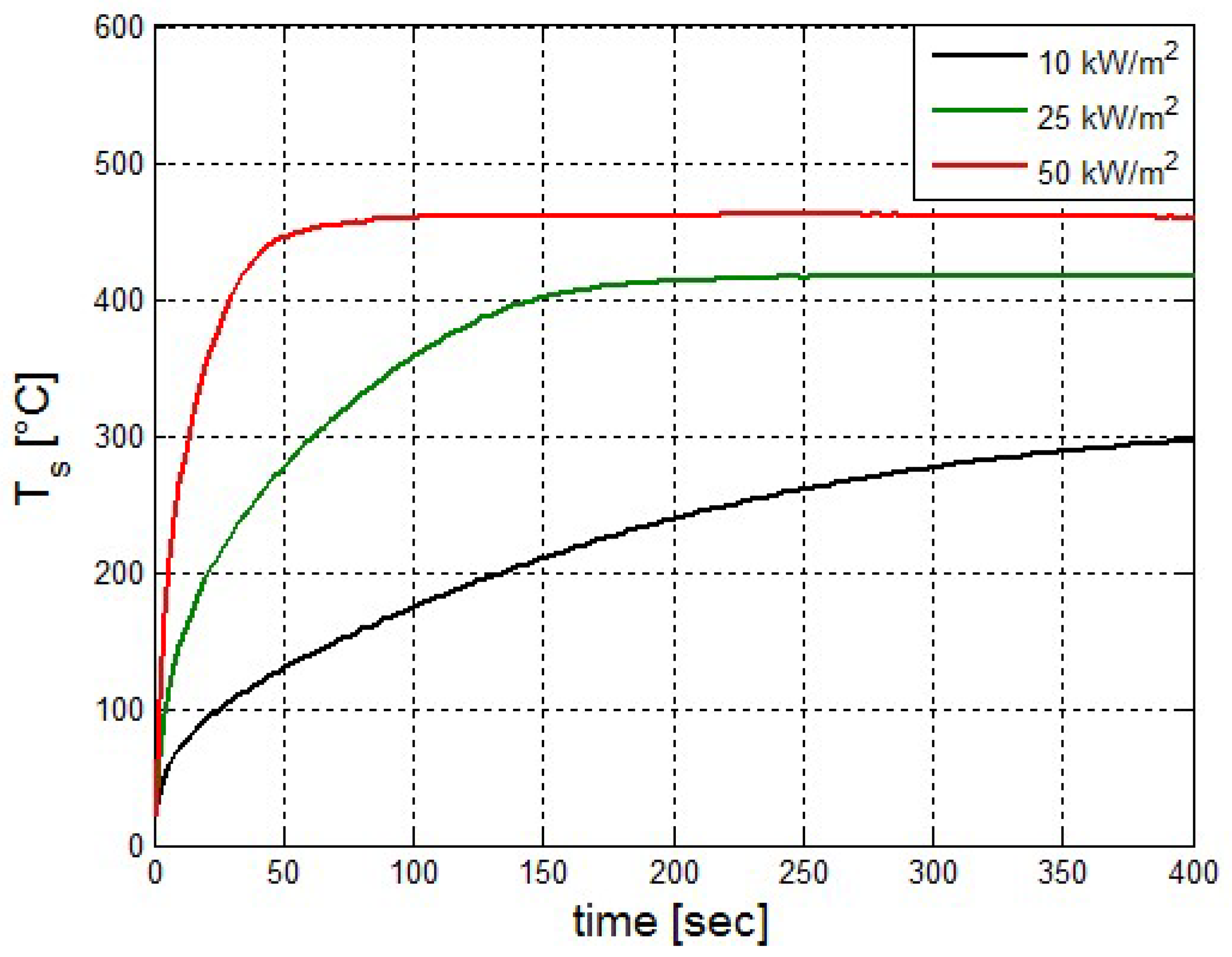
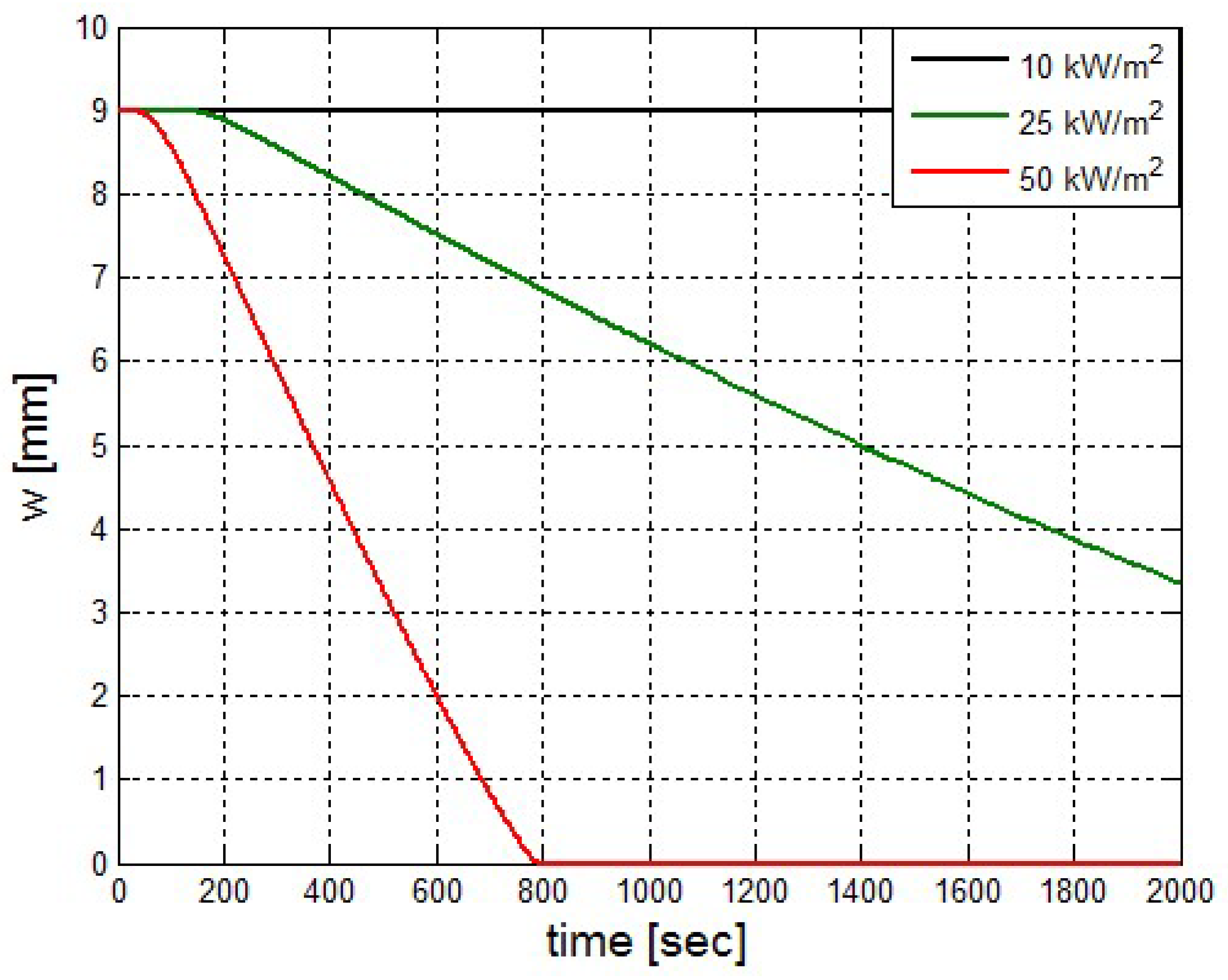
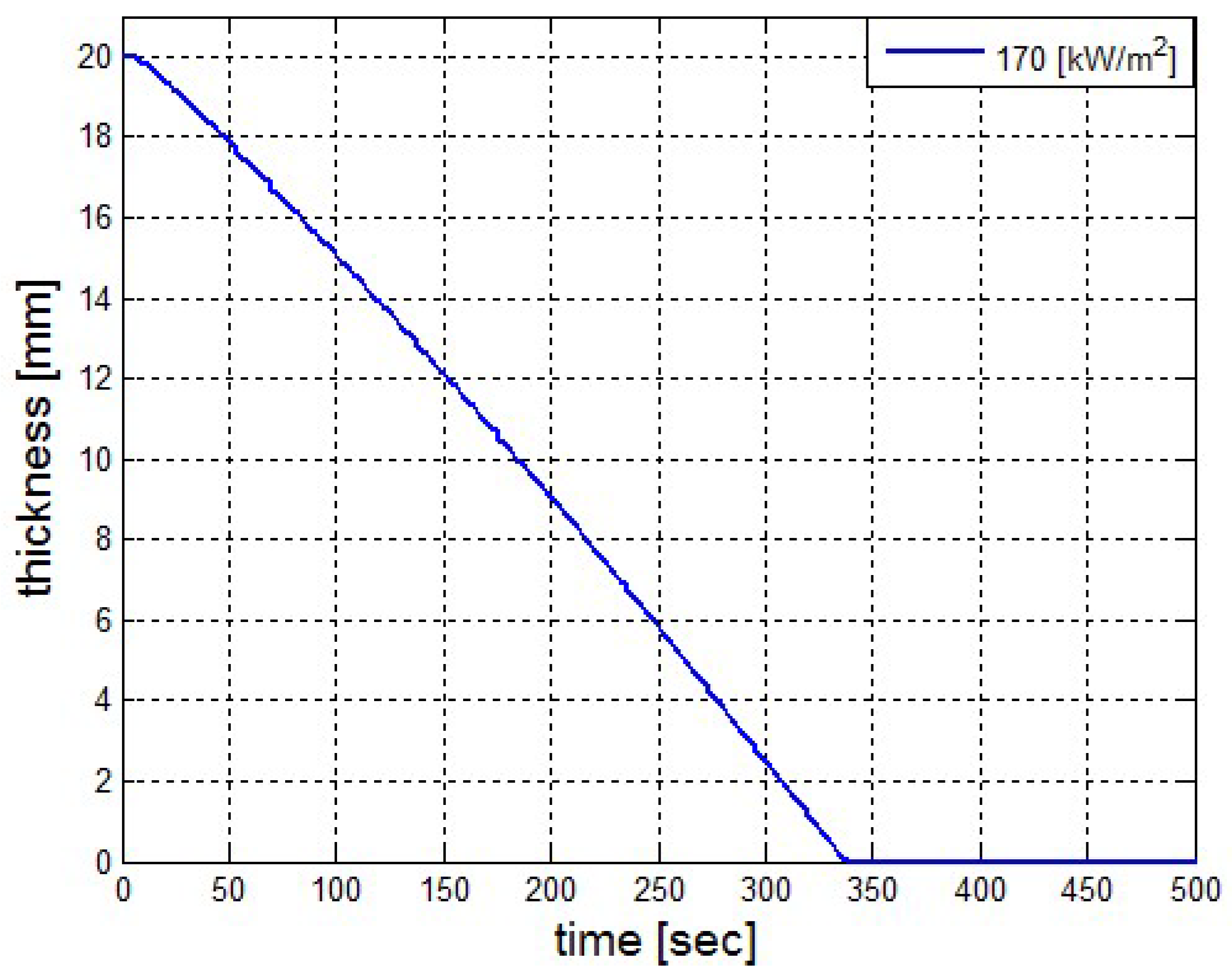
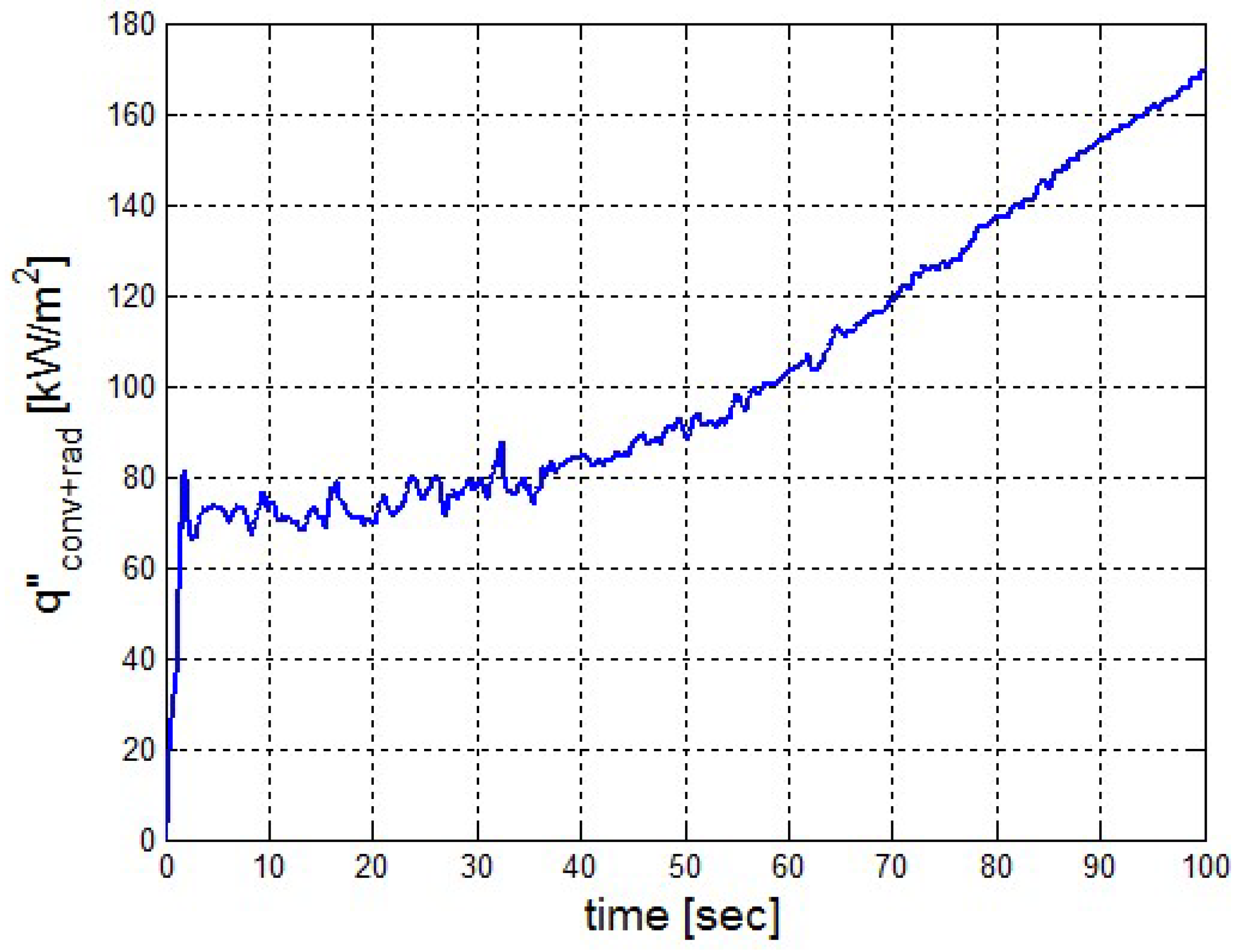
It was found that the maximal value of the combined heat flux approaches to 170 kW/m². An ablation analysis has been performed on the composite coating of the vessel. The thermophysical and thermochemical of woven glass/vinyl ester laminate have been applied in the model. The surface temperatures of the composite at different values of heat fluxes: 10 kW/m², 25 kW/m² and 50 kW/m² have been evaluated and validated. The model indicates that surface temperature of the composite increases with heat flux. Similar results for the surface temperature of the composite have been reported in the literature. It was found that for lower values of heat fluxes the erosion in the composite thickness is much smaller.

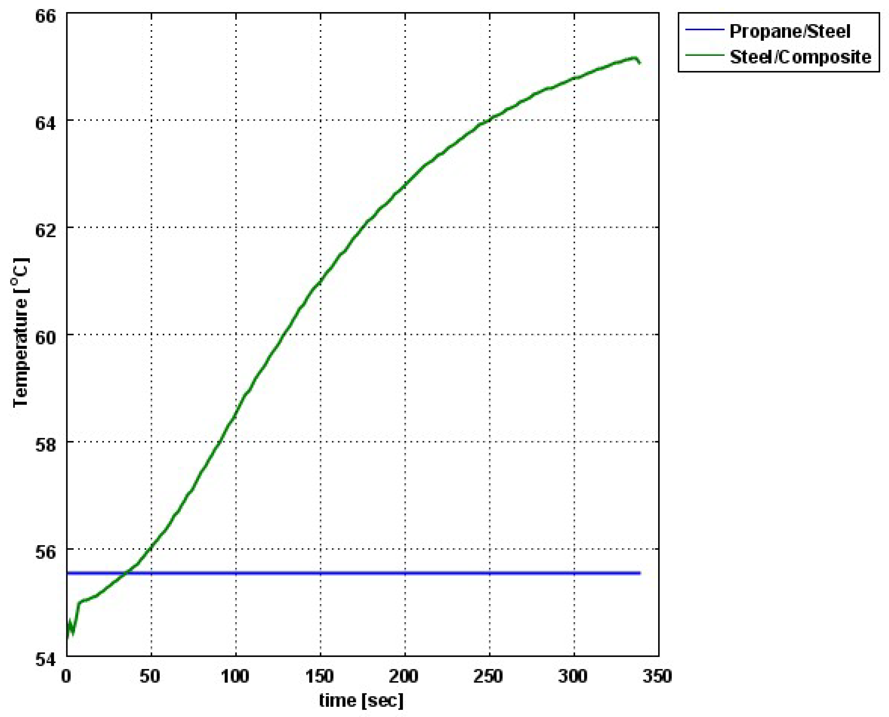
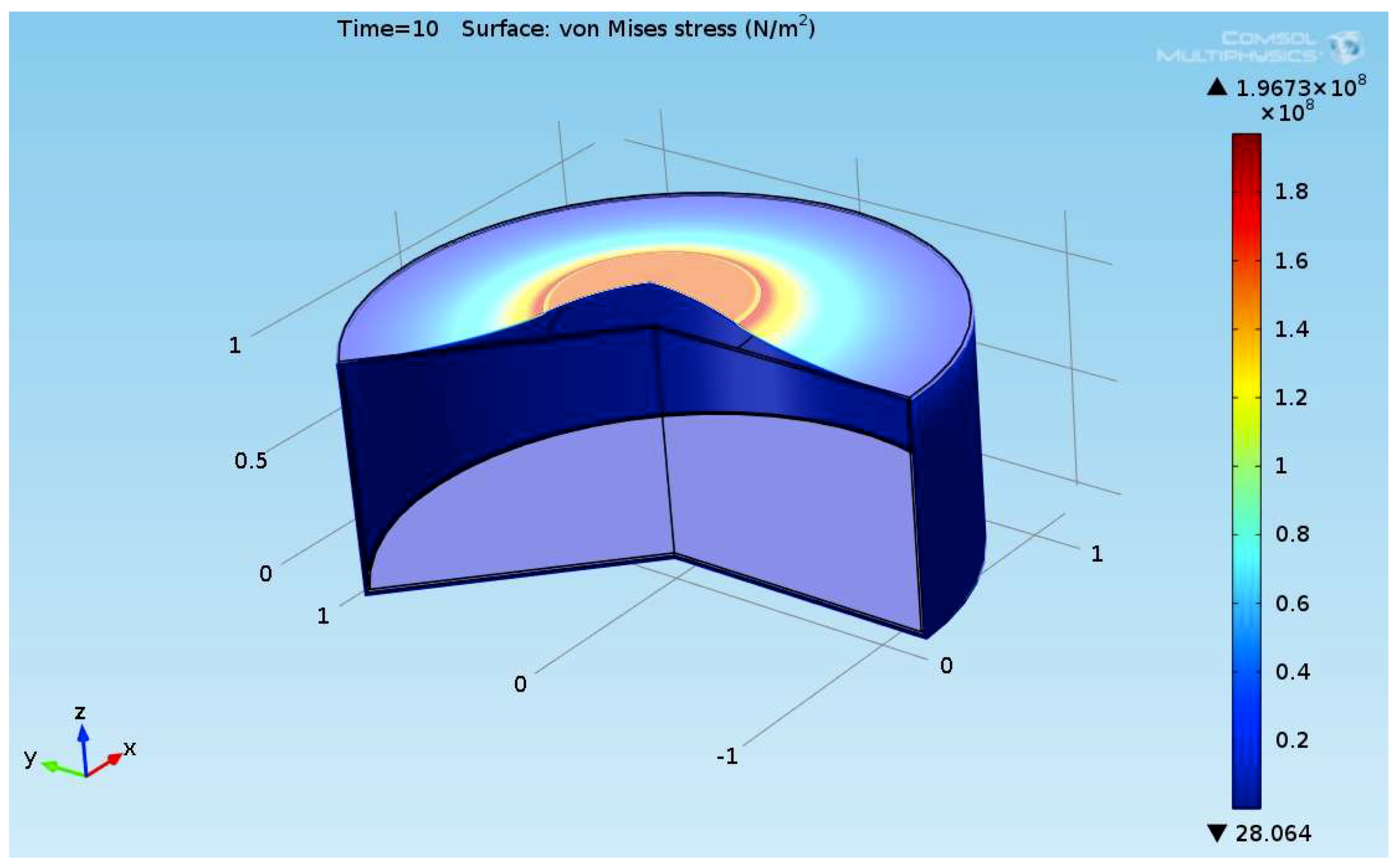
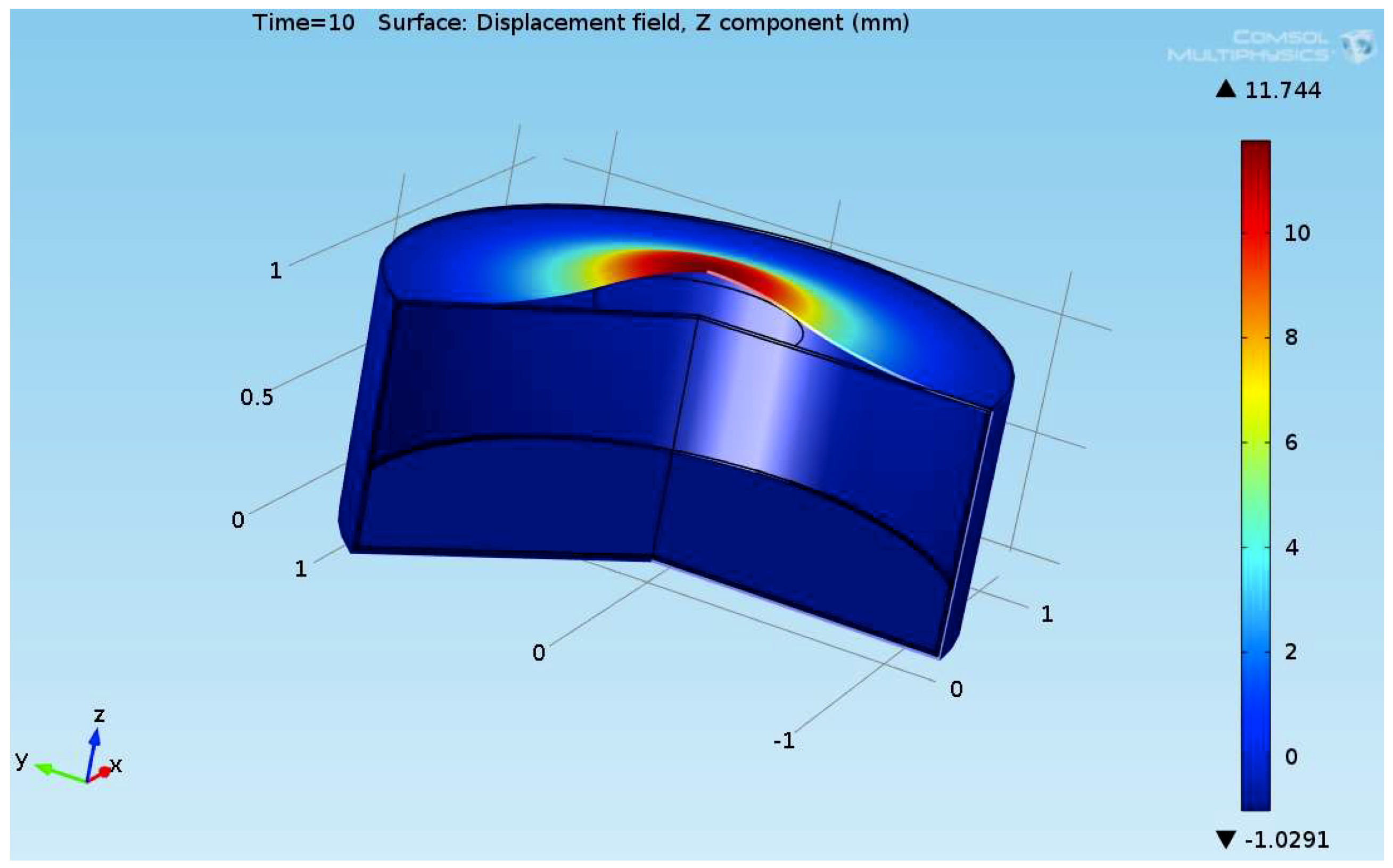
The composite eroded completely after time period of 338 s (about 6 min) for heat flux of 170 kW/m². This time period will allow to extinguish the fire or to evacuate the people in the vicinity of the accident. It should be noted that during this time period the temperature at the interface of propane/steel remains at 55.57 °C (The propane has not been heated). Since the propane is in liquid state, its convective coefficient is much larger. The temperature rise at the interface of glass-woven vinyl ester/steel is about 10 °C. The decrease in the strength of the steel can be neglected. According to the thermodynamic analysis it is shown the time period required to evaporate the liquefied propane is 22.6 min (1353.4 s). A coupled heat and structural analysis has been performed on the steel casing of the tank. The results indicate that after 10 s (after the composite lining has been eroded completely and the propane was evaporated), the maximal displacement is 11.744 mm. The maximal displacement obtained is 96% from the steel initial thickness. This value is greater than the yield point of the steel. Thus, the cover of the tank will rupture.

5. Conclusions

A new tool has been developed in this work to analyze the pressure vessel exposed to jet fire. The described work contains new tools and methods. The CFD simulation of the heptane impinging jet was carried by using the FDS (version 5).

In this work I have also modeled the recession phenomena. It should be noted that numerical modeling of thermochemical erosion is still complicated issue. The numerical modeling requires much more knowledge than the conventional approach such as: Arrhenius coefficients (the data is obtained from thermogravimetric experiments), and enthalpy of formation virgin material (the data is obtained from calorimeter experiments). As far as I know this is the first time, that the recession of the composite lining is applied on thermal protection of tank. Moreover, the FDS results have been coupled with COMSOL to extend the capabilities of the algorithm and to address other physical phenomena such as transient heating of the steel, structural analysis of the lining and steel tank as a function. The proposed algorithm is very flexible. It is possible to perform simulation of methane or other Hydrocarbon fuels. This model can be implemented for simulating other kinds of composite linings (such as PMMA, PEEK). This work can be implemented on BLEVE caused by pool fire. It is possible to add to the proposed model additional coating which will be on the glass Vinyl Coating such as intumescent coating.