Euler–Lagrange Modeling of Bubbles Formation in Supersaturated Water

Abstract

Phase transition, and more specifically bubble formation, plays an important role in many industrial applications, where bubbles are formed as a consequence of reaction such as in electrolytic processes or fermentation. Predictive tools, such as numerical models, are thus required to study, design or optimize these processes. This paper aims at providing a meso-scale modelling description of gas–liquid bubbly flows including heterogeneous bubble nucleation using a Discrete Bubble Model (DBM), which tracks each bubble individually and which has been extended to include phase transition. The model is able to initialize gas pockets (as spherical bubbles) representing randomly generated conical nucleation sites, which can host, grow and detach a bubble. To demonstrate its capabilities, the model was used to study the formation of bubbles on a surface as a result of supersaturation. A higher supersaturation results in a faster rate of nucleation, which means more bubbles in the column. A clear depletion effect could be observed during the initial growth of the bubbles, due to insufficient mixing.

1. Introduction

Bubble columns, and in general bubbly flows, represent an often encountered class of unit operations in industrial processes where contact between a gas and a liquid takes place, often in presence of chemical reaction and heat/mass transport between the phases. Despite the widespread applications of these systems, detailed understanding of the complex interactions between hydrodynamics and mass/heat transport is still insufficient, especially concerning dense flows (heterogeneous regime) and their effect on the large-scale performance of bubble column reactors [1,2]. The use of Computational Fluid Dynamics (CFD) to model and study these systems is becoming more and more widespread resulting from large improvements in computational power. Different levels of detail (length scales) can be identified ranging from large scale Euler–Euler simulations to detailed Direct Numerical Simulations (DNS). At an intermediate level, Euler–Lagrange models, where each bubble is tracked individually in a Lagrangian manner, play an important role in gaining details on the behaviour of bubble swarms with a relatively large number of bubbles [3].

Phase transition as a consequence of supersaturation occurs in a variety of natural and industrial processes. A well known example is opening a bottle of soda: the sudden change in pressure creates a local supersaturation and bubbles form on the surface of the bottle. Another mechanism to obtain local supersaturation is when a reaction produces gas in excess. Relevant industrial applications are in electrolytic processes where gas (such as H${}_2$ in the electrolysis of brine) bubbles are formed on the electrodes [4,5], carbonated beverages [6], molten polymers [7] and even bubbles in oil reservoirs [8]. CFD models describing the hydrodynamics of a system where bubbles are formed are thus very relevant for industry, but their capabilities are often yet inadequate in practice.

Often, Eulerian–Eulerian models include a gas generation term as a boundary condition and information about the bubble sizes can be obtain through the implementation of a nucleation rate in a Population Balance Model (PBM) [9]. Examples of the use of these models can be found in the context of electrochemical reactions, where gasses are produced on electrodes. For instance, Liu et al. [10] used the Two Fluid Model to simulate the electrochemical oxidation of p-methoxyphenol while El-Askary et al. [11] simulated the production of hydrogen in an electrochemical cell. On the other hand, detailed DNS models are limited by the computational cost. Liu et al. [12] used a Volume of Fluid (VOF) model to simulate a single gas bubble growing in the water electrolysis process. In their study, they noted the strong analogy between boiling and bubble formation in supersaturated liquids. Many studies have been done for boiling flows, especially using VOF [13,14] and Lattice–Boltzmann methods [15], but this goes beyond the scope of this work. Regarding supersaturation, those methods has been applied for instance by Liu et al. [12], but it is possible to even find detailed Molecular Dynamics (MD) simulations of nano-bubbles nucleation [16].

In the framework of multi-scale modeling, as presented by van Sint Annaland et al. [3], the meso-scale remains important to close the gap between the two large scales and the micro-scale, not only for bubbly flows as such, but also for flows with nucleating bubbles. It is crucial, for instance, to quantify nucleation rates for use in larger scale models or to quantify surface coverage as a consequence of bubble formation, because electro-chemical processes can be severely hampered by the bubbles formed on electrode surfaces. Detailed experiments on bubble nucleation have been done at the micro-scale (e.g., by van der Linde et al. [17], who showed gas depletion due to nucleating bubbles on a micro-structured surface with a single nucleation point), but not many studies have focused on multiple bubbles nucleation at the meso-scale, including mass transfer limitations.

Mandin et al. [18] introduced a Lagrangian tracking for a vertical electrode, but the gas injection was modeled based on a given mass flow rate. Nierhaus et al. [19] used a two-way coupled Euler–Lagrange model to study hydrogen bubble formation in a rotating electrode configuration. In their work they applied at the gas inlet a pre-defined bubble size distribution obtained from experimental data. In their group, they subsequently improved the model: first van Parys et al. [20] introduced a model of bubble growth on a surface by supersaturation, and after van Damme et al. [21] introduced nucleation sites, although the detachment radius is fixed in their simulations. More recently, Hreiz et al. [22] used the Euler–Lagrange model of ANSYS Fluent to simulate a vertical electrode. They treated the nucleation sites as injection points, recognizing in their work that a more sophisticated approach for bubble nucleation/injection in the system is required. The novelty of this work relies in the new proposed nucleation algorithm which considers discrete nucleation sites with distinct properties and links it to the hydrodynamics of the Euler–Lagrange model and to the classical nucleation theory, as an improvement of the work of van Damme et al. [21].

The aim of this work was thus to develop an Eulerian–Lagrangian model to simulate at the meso-scale bubbly flows where phase transition via supersaturation occurs. In the following sections, the developed model and the numerical setup are described and verified. Then, results of preliminary simulations on bubble formation due to supersaturation by heterogeneous nucleation are described to demonstrate the model’s capabilities.

2. Model Description

The Discrete Bubble Model (DBM) is a Euler–Lagrange type of CFD model, based on the work of Delnoij et al. [23] subsequently expanded and improved by Darmana et al. [1] and Lau et al. [24]. Newton’s laws of motion are used to track each individual bubble, while accounting for bubble–bubble interactions (collisions, coalescence and breakup), mass transport and in this work also phase transition. A detailed description of the model will be given in the following sections. For more details, the interested reader is referred to the cited works [1,23,24].

2.1. Liquid Dynamics

The fluid flow is described by the volume-averaged Navier–Stokes equations:

$$\begin{array}{c}\frac{\partial }{\partial t}\left({\rho }_l{\alpha }_l\right)+\nabla ·{\rho }_l{\alpha }_l\mathbf{u}=\dot{M}\\ \frac{\partial }{\partial t}\left({\rho }_l{\alpha }_l\mathbf{u}\right)+\nabla ·\left({\rho }_l{\alpha }_l\mathbf{u}\mathbf{u}\right)=-{\alpha }_l\nabla p+{\alpha }_l\rho \mathbf{g}+\nabla ·{\alpha }_l{\mathit{\tau }}_l+\mathsf{\Phi }\end{array}$$

(1)

where $\mathbf{u}$ is the fluid velocity, ${\alpha }_l$ denotes the liquid fraction, $\mathsf{\Phi }$ represents the momentum coupling between the liquid and the discrete gas phase and $\dot{M}$ is the volumetric mass exchange rate. In this equation, $\mathbf{\tau }$ represents the stress tensor, which is described for incompressible Newtonian fluids by:

$${\mathit{\tau }}_l=-{\mu }_{\mathrm{eff}}\left[\nabla \mathbf{u}+{(\nabla \mathbf{u})}^T-\frac{2}{3}\mathit{I}(\nabla ·\mathbf{u})\right]$$

(2)

The effective viscosity ${\mu }_{\mathrm{eff}}$, calculated as in Equation (3), includes the contribution of the LES sub-grid scale turbulent viscosity (${\mu }_T$).

$${\mu }_{\mathrm{eff}}={\mu }_l+{\mu }_T$$

(3)

The turbulent viscosity is calculate using the model developed by Vreman [25]:

$${\mu }_T=2.5{\rho }_l{C}_S^2\sqrt{\frac{B_{\beta }}{{\alpha }_{ij}{\alpha }_{ij}}}$$

(4)

where ${\alpha }_{ij}=\frac{\partial u_j}{\partial x_i}$, $B_{\beta }={\beta }_{11}{\beta }_{22}-{\beta }_{12}^2+{\beta }_{11}{\beta }_{33}-{\beta }_{13}^2+{\beta }_{22}{\beta }_{33}-{\beta }_{23}^2$ and ${\beta }_{ij}={\Delta }_m^2{\alpha }_{mi}{\alpha }_{mj}$. The constant $C_S$ represents the Smagorinsky constant and is set to a value of 0.1, while ${\Delta }_i$ is the filter width in the i direction.

2.2. Bubble Dynamics

With Newton’s laws of motion, each bubble is tracked, accounting for the different forces acting on it. The motion of the bubbles can be described with:

$$\begin{array}{c}{\rho }_b{V}_b\frac{d\mathbf{v}}{dt}=\sum \mathbf{F}-\left({\rho }_b\frac{d{V}_b}{dt}\right)\mathbf{v}\\ \frac{d{\mathbf{x}}_b}{dt}=\mathbf{v}\end{array}$$

(5)

where $\mathbf{v}$ represents the bubble velocity and ${\mathbf{x}}_b$ its position in the 3D domain. The sum of the forces on bubbles is composed of buoyancy, drag [26,27], lift [28], virtual mass [29] and wall-interactions [30], as given by Equation (6):

$$\sum \mathbf{F}={\mathbf{F}}_G+{\mathbf{F}}_P+{\mathbf{F}}_D+{\mathbf{F}}_L+{\mathbf{F}}_{VM}+{\mathbf{F}}_W$$

(6)

An overview of the different closure relations used for the forces is given in

Table 1. Forces acting on a bubble.

Force	Closure Relation	References
${\mathbf{F}}_G={\rho }_b{V}_b\mathbf{g}$	-	-
${\mathbf{F}}_P=-V_b\nabla P$	-	-
${\mathbf{F}}_D=-\frac{1}{2}{C}_D{\rho }_l\pi R_b^2\left|\mathbf{v}-\mathbf{u}\right|\left(\mathbf{v}-\mathbf{u}\right)$	$\frac{C_D}{C_{D,\infty }}=\left(1+\frac{18}{\mathrm{E}\ddot{\mathrm{o}}}{\alpha }_b\right){\alpha }_l$	[26,27]
	$C_{D,\infty }=\sqrt{C_{D,\infty }{\left(\mathrm{Re}\right)}^2+C_{D,\infty }{\left(\mathrm{E}\ddot{\mathrm{o}}\right)}^2}$
	$C_{D,\infty }\left(\mathrm{Re}\right)=\frac{16}{\mathrm{Re}}\left(1+\frac{1}{1+\frac{16}{\mathrm{Re}}+\frac{3.315}{\sqrt{\mathrm{Re}}}}\right)$
	$C_{D,\infty }\left(\mathrm{E}\ddot{\mathrm{o}}\right)=\frac{4\mathrm{E}\ddot{\mathrm{o}}}{\mathrm{E}\ddot{\mathrm{o}}+9.5}$
${\mathbf{F}}_L=-C_L{\rho }_l{V}_b\left(\mathbf{v}-\mathbf{u}\right)\times \left(\nabla \times \mathbf{u}\right)$	$C_L=\left\{\begin{array}{cc}min[0.288tanh\left(0.121\mathrm{Re}\right),f\left(\mathrm{E}{\ddot{\mathrm{o}}}_d\right)]\hfill & \mathrm{E}\ddot{\mathrm{o}}<4\hfill \\ f\left(\mathrm{E}{\ddot{\mathrm{o}}}_d\right)4\le \mathrm{E}\ddot{\mathrm{o}}\hfill & \le 10\hfill \\ -0.29\hfill & \mathrm{E}\ddot{\mathrm{o}}>10\hfill \end{array}\right.$	[28]
	$f\left(\mathrm{E}{\ddot{\mathrm{o}}}_d\right)=0.00105\mathrm{E}{\ddot{\mathrm{o}}}_d^3-0.0159\mathrm{E}{\ddot{\mathrm{o}}}_d^2-0.0204\mathrm{E}{\ddot{\mathrm{o}}}_d+0.474$
	$\mathrm{E}{\ddot{\mathrm{o}}}_d=\frac{\mathrm{E}\ddot{\mathrm{o}}}{E_b},E_b=\frac{1}{1+0.163\mathrm{E}{\ddot{\mathrm{o}}}^{0.757}}$
${\mathbf{F}}_{VM}=-C_{VM}{\rho }_l{V}_b\left(\frac{D\mathbf{v}}{Dt}-\frac{D\mathbf{u}}{Dt}\right)$	$C_{VM}=0.5$	[29]
$\begin{array}{l}{\mathbf{F}}_W=-C_W{R}_b\left(\frac{1}{y^2}-\frac{1}{{(L-y)}^2}\right)\\ {\rho }_l{\left|\left(\mathbf{v}-\mathbf{u}\right)·{\mathbf{n}}_z\right|}^2{\mathbf{n}}_w\end{array}$	$C_W=\left\{\begin{array}{c}\begin{array}{cc}\hfill e^{\left(-0.933\mathrm{E}\ddot{\mathrm{o}}+0.179\right)}& 1\le \mathrm{E}\ddot{\mathrm{o}}\le 5\hfill \\ \hfill 0.007\mathrm{E}\ddot{\mathrm{o}}+0.04& 5\le \mathrm{E}\ddot{\mathrm{o}}\le 33\hfill \end{array}\hfill \end{array}\right.$	[30]

. These closures were selected following the work of Lau et al. [24] and have been used in several works, within our group [1,24,31] as well as outside [32,33,34]. The interphase two-way coupling is performed through a polynomial mapping in order to map quantities between the Eulerian grid and the Lagrangian bubbles. The chosen technique is a clipped fourth-order polynomial following the work of Deen et al. [35].

An important aspect is the volume change due to the interphase mass transfer. This is accounted for as:

$${\rho }_b\frac{d{V}_b}{dt}=\dot{m}$$

(7)

It is relevant to note that the virtual mass force should account for the contribution of the changing volume of the bubble, $\rho C_{VM}\frac{d{V}_b}{dt}(\mathbf{u}-\mathbf{v})$, as described by Magnaudet and Eames [36]. This contribution is important even when the relative velocity does not change with time, if the bubble is shrinking or growing. Here, this contribution has been neglected as the main purpose is the nucleation model demonstration. Moreover, the fastest rate of volume change happens when the bubble is still attached to the surface. In this case, forces are not calculated, as explained further in Section 2.5.3, which allows safely excluding this term for such bubbles. However, when the bubble is freely rising in the column, even at its steady-state velocity, the contribution of the virtual mass force due to growth can become the same order of magnitude as the drag force for the fastest growing bubbles. This implies that this term should be included in cases where the dynamics of freely rising bubbles is important.

More details on the gas–liquid mass exchange rate are given in the following sections.

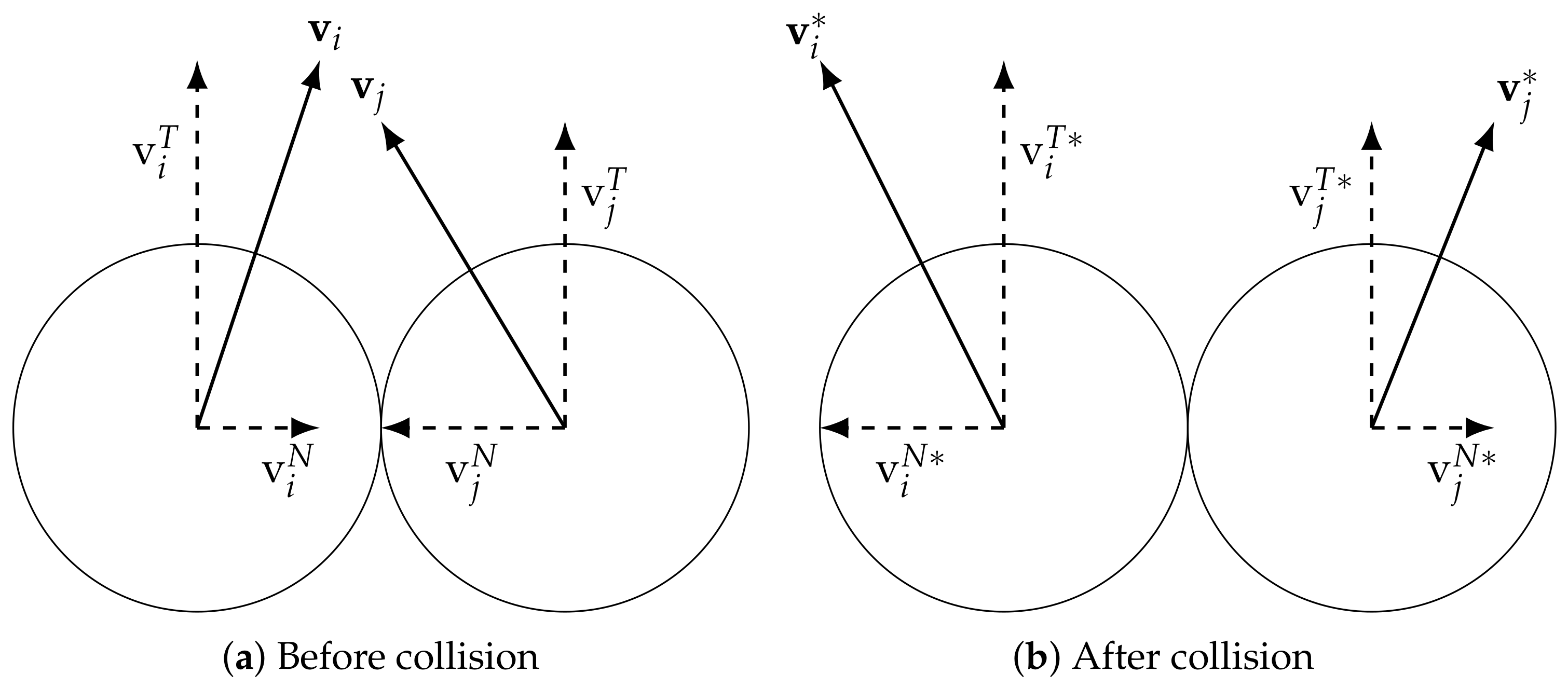
2.2.1. Bubble Interactions

As mentioned in the previous section, bubble collisions, coalescence and breakup have been taken into account in the model. The position, velocity and size of each bubble are already available as they are obtained during the simulation, allowing for an easy detection of binary encounters with other bubbles or with the wall. The collision model used in this work is based on the hard-sphere approach of Hoomans et al. [37] and its adaptation from Delnoij et al. [23], where collisions are event-based and are considered as perfectly elastic. To speed up the calculation routines, a neighbour list concept as described by Darmana et al. [1] is used. When bubbles are colliding (assuming bubbles i and j collide, as visible in Figure 1), the tangential velocity component (${\mathrm{v}}_i^T$) remains unchanged, while the new normal component (${\mathrm{v}}_i^{N_{\ast }}$) is calculated as:

$${\mathrm{v}}_i^{N_{\ast }}=2\frac{m_i{\mathrm{v}}_i^N+m_j{\mathrm{v}}_j^N}{m_i+m_j}-{\mathrm{v}}_i^N$$

(8)

When the collision is evaluated, the size change of the bubble as a result of mass transfer needs to be accounted for. In the cases considered in this paper, the supersaturation of the liquid results in sometimes faster rates of bubble growth than the velocity of the bubble itself. Two bubbles that are slowly moving apart could still collide if their sizes are growing fast. To accurately resolve these situations, the bubble size rate of growth $\dot{R}$ has been included in the impulse calculation for the collision [1].

In addition to elastic collisions, bubbles can coalesce and merge into a bigger one when in contact for enough time. Many theories and models exist for bubble coalescence (see Lau et al. [24]). In this work, the film drainage model as implemented by Darmana et al. [1] is used. Two colliding bubbles trap a thin film of liquid between them, which can drain over time. If the two gas elements are in contact for sufficiently long time, it will completely drain allowing coalescence. This can be modelled with:

$$t_{\mathrm{contact}}\ge t_{\mathrm{drainage}}$$

(9)

Prince and Blanch [38] calculated the drainage time as:

$$t_{\mathrm{drainage}}=\sqrt{\frac{d_{eq}^3{\rho }_l}{128\sigma }}\ln \frac{{\theta }_0}{{\theta }_f}$$

(10)

where ${\theta }_0$ and ${\theta }_f$ represent, respectively, the initial and final film thickness during the drainage process, which are equal to 1 × 10${}^{-4}$ $\mathrm{m}$ and 1 × 10${}^{-8}$ $\mathrm{m}$, respectively [1]. The contact time of the two bubbles is calculated through the correlation proposed by Sommerfeld et al. [39], assuming that it is proportional to a deformation distance divided by the normal component of the two absolute relative velocity of the bubbles, as described in Equation (11):

$$t_{\mathrm{contact}}=\frac{C_{\mathrm{co}}{d}_{\mathrm{eq}}}{2\left|{\mathrm{v}}_i^N-{\mathrm{v}}_j^N\right|}$$

(11)

The deformation distance is in essence the distance that the two centres of mass move further towards each other, starting from the sum of the two radii (zero deformation, perfect spheres) when bubbles deform. Since deformation is difficult to quantify, it is calculated as a fraction of the equivalent diameter. Indeed, the coalescence constant (C${}_{\mathrm{co}}$), which is set to a value of 0.5, represents the deformation distance normalized by the effective bubble diameter and should be treated as a calibration parameter. For a detailed description of the deformation process, the reader is referred to the work of Sommerfeld et al. [39]. When both the film drainage and contact time are calculated, with Equation (9), it is possible to distinguish between simple elastic collision or coalescence, i.e., at the step of Figure 1a. In the latter eventuality, the resulting bubble will have a volume, or mass as it is considered as incompressible, equal to the sum of the two parents.

Bubbles rising in a liquid can also break as a consequence of various factors, such as turbulent fluctuations, viscous shear stress, surface instabilities, etc. [40]. The break-up model implemented in the DBM is based on the work of Lau et al. [24]: this model assumes that break-up occurs when the inertial forces acting on the bubble (which deform the bubble) are larger than the surface tension force. Based on a force balance, a critical Weber number is used as a criterion for the break-up of spherical bubbles:

$$\mathrm{We}=\frac{{\rho }_l\overline{\delta u^2\left(d\right)}{d}_{\mathrm{eq}}}{\sigma }\ge 12$$

(12)

where $\overline{\delta u^2\left(d\right)}$ represents the mean square velocity difference at the distance of the bubble diameter [24]. The break-up is considered to be binary, forming only two daughter bubbles with a size taken from a U shaped daughter size distribution. The resulting bigger bubble is assigned the parent’s original position while the smaller is randomly placed around the other, at a distance of $1.1$ times the sum of their radii, preventing overlap and immediate coalescence of the two daughter bubbles (see [24]).

2.3. Species Transport and Mass Transfer

The Discrete Bubble Model includes the species transport equations accounting for mass transfer and chemical reaction. A transport equation for each species is implemented on the same Eulerian grid as the momentum equations as:

$$\frac{\partial }{\partial t}\left({\alpha }_l{\rho }_l{Y}_l^j\right)+\nabla ·\left({\alpha }_l\left({\rho }_l\mathbf{u}{Y}_l^j-{\Gamma }_{\mathrm{eff}}^j\nabla Y_l^j\right)\right)=\dot{M}+{\alpha }_l{S}^j$$

(13)

where $Y_l^j$ represents the mass fraction of component j in the liquid phase, $S^j$ is its source/sink term accounting for chemical reactions, $\dot{M}$ represents the net volumetric mass transfer rate between the phases and ${\Gamma }_{\mathrm{eff}}$ is the effective dispersion coefficient, calculated as:

$${\Gamma }_{\mathrm{eff}}^j={\rho }_l{\mathcal{D}}_l^j+\frac{{\mu }_T}{{\mathrm{Sc}}_T^j}$$

(14)

In Equation (14), the turbulent Schmidt number is approximated to ${\mathrm{Sc}}_T^j=1$ [31]. Equation (13) is solved for $N_S-1$ components. The last component, usually the solvent (e.g., water), is evaluated by enforcing the summation equation:

$$\sum _{j=1}^{N_S}{Y}_l^j=1$$

(15)

The physical properties of the mixture are calculated as the weighted average of each species. The interphase mass transfer rate is a function of the concentration difference between the bubble (assumed to be composed entirely of one gas, namely CO₂, thus neglecting evaporation of the liquid) and the liquid. This has been expressed by Darmana et al. [1] as:

$${\dot{m}}_b^j=k_l^j{A}_b{\rho }_l\left(Y_l^{j^{\ast }}-Y_l^j\right)$$

(16)

The mass transfer coefficient is determined by a Sherwood relation valid for spherical gas bubbles [41]:

$$\mathrm{Sh}=2+0.6415{\left(\mathrm{Re}{\mathrm{Sc}}^j\right)}^{\frac{1}{2}}$$

(17)

The gas side mass fraction is calculated from the Henry constant:

$$Y_l^{j^{\ast }}=H^j{Y}_b^j\frac{{\rho }_b}{{\rho }_l}$$

(18)

The transport equation is discretized implicitly (with a semi-implicit source term for the reaction) on the Eulerian grid and the resulting linear system is solved using a biconjugate gradient method implemented in the scientific library PETSc [42,43].

2.4. Verification

The hydrodynamics of the DBM has been validated in the past by Lau et al. [24], with the use of experimental data from a square bubble column, performed by Deen et al. [44]. On the other hand, the species solver has been modified since [1], and a verification with benchmark analytical cases is required to assess the numerical validity of the results. A few unidirectional verification cases have been performed, as will be detailed in the following sections.

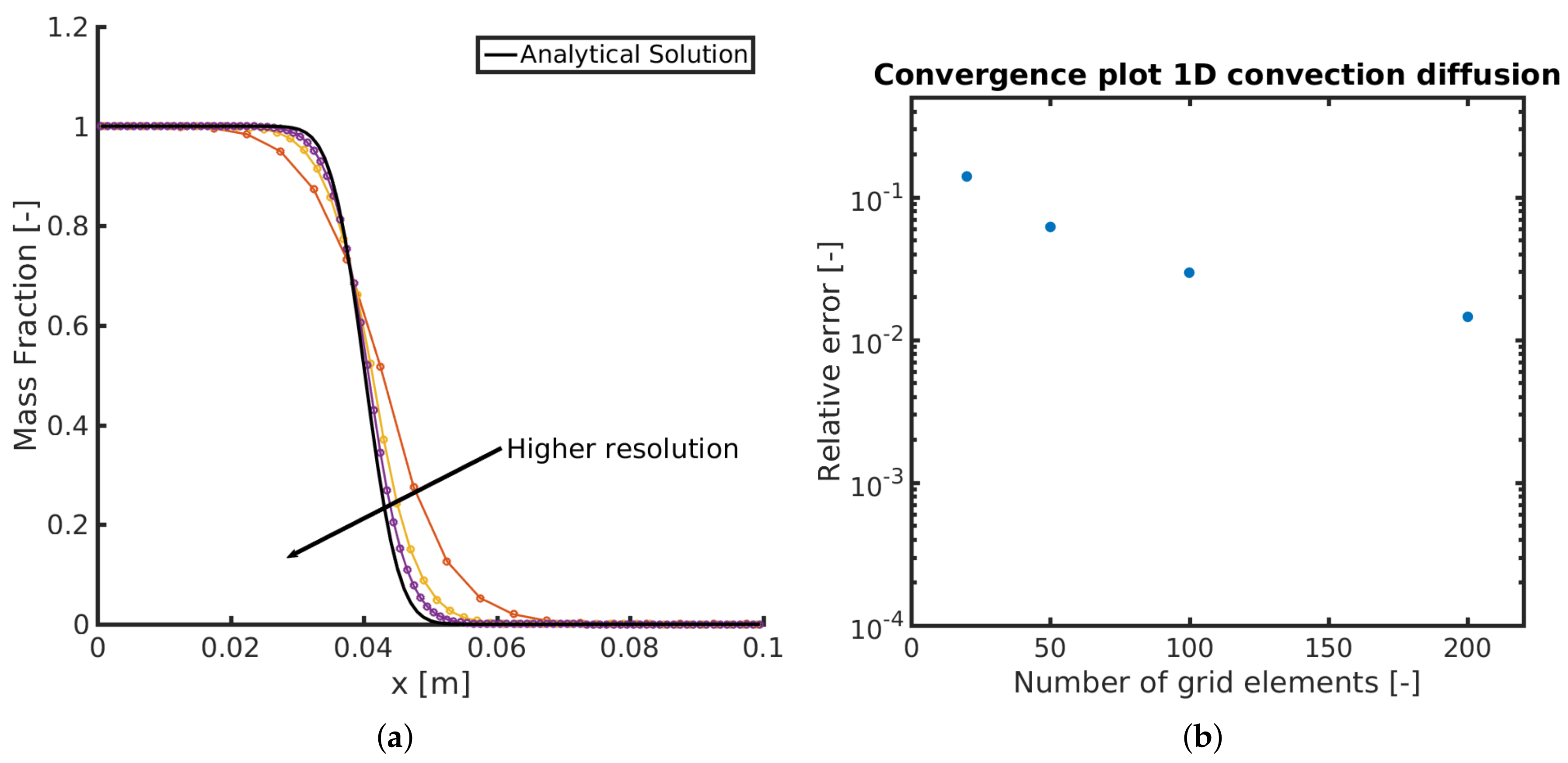
2.4.1. 1D Convection-Diffusion

In this case, a unidirectional flow in the domain is considered where the concentration of the component of interest is initially zero. The density is assumed constant. A flow from one side (where the mass fraction is $Y_l=1$) is started and diffusion takes place. Equation (13) simplifies to:

$$\frac{\partial c}{\partial t}+u\frac{\partial c}{\partial x}=\mathcal{D}\frac{{\partial }^{2}c}{\partial x^2}$$

(19)

The analytical solution for this system has been derived by Ogata and Banks [45] as:

$$\begin{array}{c}\hfill \frac{c}{c_0}=\frac{1}{2}\left[\mathrm{erfc}\left(\frac{x-ut}{2\sqrt{\mathcal{D}t}}\right)+\exp \left(\frac{ux}{\mathcal{D}}\right)\mathrm{erfc}\left(\frac{x+ut}{2\sqrt{\mathcal{D}t}}\right)\right]\end{array}$$

(20)

In Figure 2a, it is shown that the grid resolution plays an important role (due to the well known numerical diffusion) but the solver approaches very well the analytical solution at sufficiently high number (200 in this case) of grid elements. As visible in Figure 2b, the error reduces linearly increasing the number of grid sizes.

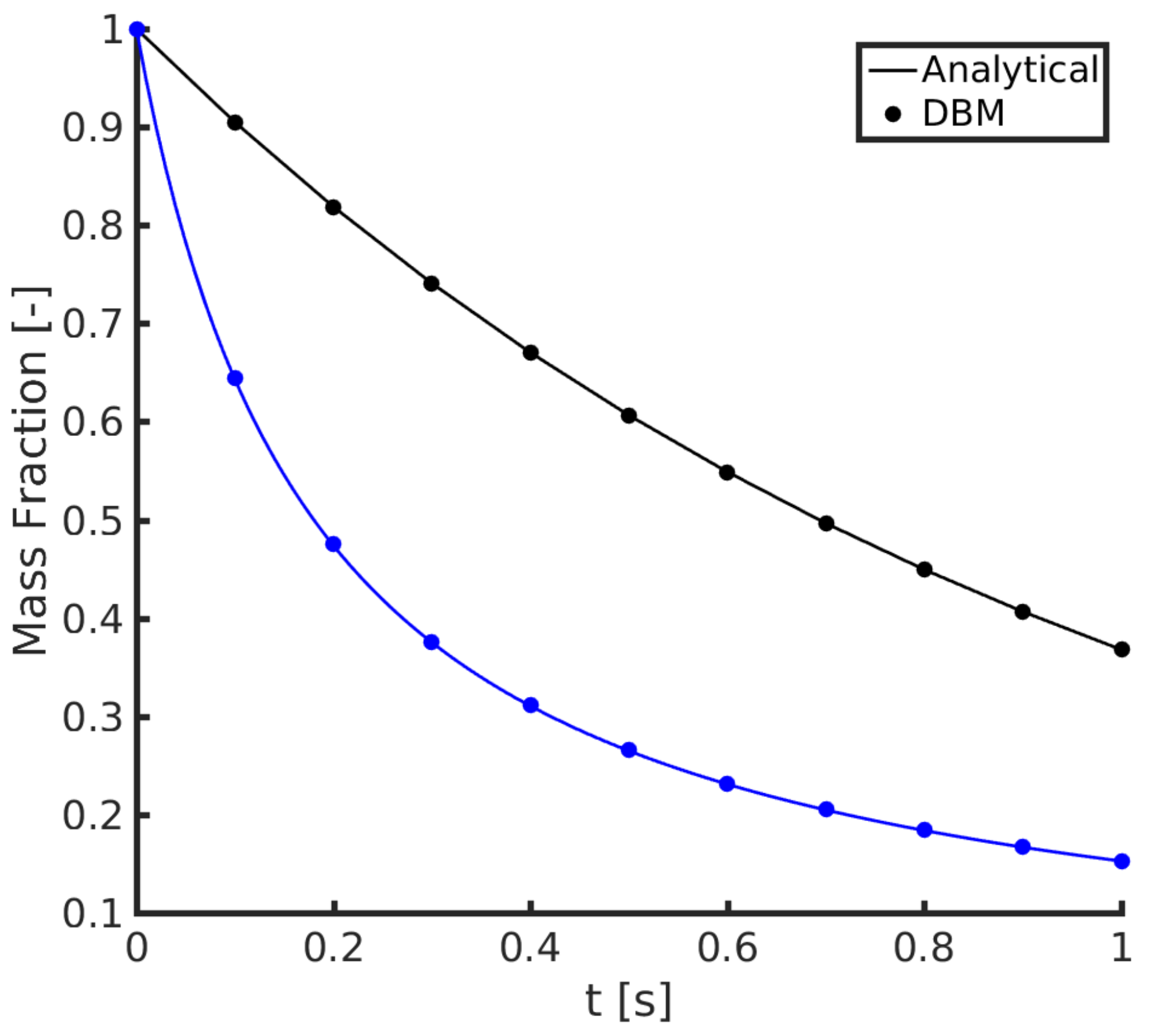
2.4.2. Batch Reaction

To verify the correct implementation of the semi-implicit discretization for the source/sink term and mass transfer, a simple reaction $A\to B$ is implemented with a first and a second order kinetics, assuming an ideally mixed batch reactor. In this case, Equation (13) simplifies to:

$$\frac{dc}{dt}=R=\left\{\begin{array}{cc}-k_{R}c\hfill & 1\mathrm{st}\mathrm{order}\mathrm{reaction}\hfill \\ -k_R{c}^2\hfill & 2\mathrm{nd}\mathrm{order}\mathrm{reaction}\hfill \end{array}\right.$$

(21)

where $k_R$ represents the reaction rate. Integration of Equation (21) yields to the analytical solutions:

$$c=\left\{\begin{array}{cc}{c}_0\exp (-k_{R}t)\hfill & 1\mathrm{st}\mathrm{order}\mathrm{reaction}\hfill \\ \frac{1}{1/c_0+k_{R}t}\hfill & 2\mathrm{nd}\mathrm{order}\mathrm{reaction}\hfill \end{array}\right.$$

(22)

As shown in Figure 3, the DBM results match very well with the analytical solutions.

2.5. Phase Transition

2.5.1. Theoretical Overview

An important concept is supersaturation: a liquid is (locally) supersaturated when the concentration is higher than the equilibrium concentration, which can be expressed, for instance, by Henry’s law as done in Equation (18). A relevant parameter, called the supersaturation ratio, is introduced as [46]:

$$\zeta =\frac{c}{c_s}-1$$

(23)

It indicates that, for phase transition to occur, $\zeta >0$. Equilibrium between the two phases exists when this ratio is equal to 0.

The mechanism of a gas bubble formation has been a topic of investigation for many years [47]. Two different macro classes are generally distinguished: homogeneous and heterogeneous nucleation. In their review, Jones et al. [47] identified four different types of bubble nucleation mechanisms:

Type I:

The classical homogeneous nucleation, i.e., the spontaneous creation of a bubble in the liquid bulk. This mechanisms is characterized by the high energy requirements to form a new gas–liquid interface and the necessity to have enough gas molecules in close proximity to each other. For these reasons, only a system which exceeds a supersaturation ratio of 100 is able to form bubbles, which is extremely large. For example, for common drinks such as soda and champagne, $\zeta$ typically ranges from 2 to 5, which would mean it is impossible to have Type I nucleations for such systems [6,46].

Type II:

The classical heterogeneous nucleation. This mechanism assumes that the new interface is created in small cavities or imperfections at a solid surface (such as a wall or suspended impurities). However, a new interface still has to be created, so that supersaturation levels comparable with the homogeneous nucleation are required.

Type III/IV:

Pseudo-classical and non-classical nucleation, respectively. These two types represent the vast majority of the nucleation events in liquids with low supersaturation. Both mechanisms account for a pre-existing gas pocket, for instance as a consequence of another type of nucleation event (e.g., Type II) or simply because of the inability of the liquid to fully fill cavities on a surface. The difference between these two types lies in the geometry of the cavity. It is worth mentioning that the energy requirement for both types is respectively low and zero, meaning that Type IV is the one responsible for the long term cycle of bubble production in carbonated drinks. In this case, the production of bubbles will continue until the critical radius, increasing as a consequence of the depletion of gas in the liquid, reaches a value equal to the radius of the cavity meniscus and thus nucleation stops.

As introduced in the previous paragraph, the size of the nucleation site is crucial in describing the formation and growth of a bubble for the case of the most common mechanism Type IV. Only nucleation sites with a radius larger than a critical value [47] (related to the Laplace pressure) can host a growing bubble. This radius represents the minimum size of a bubble that is able to grow by mass transfer, without dissolving back in the liquid, and is defined as:

$$R_c=\frac{2\sigma }{p_s\zeta }$$

(24)

where $\sigma$ and $p_s$ represent the surface tension coefficient and the saturation pressure of the gas, respectively. In addition, there is a second property influencing bubble formation: the depth of the nucleation site with respect to its width/radius. As mentioned before, while pouring the (supersaturated) liquid into a vessel, flask or glass, a liquid front will move across the solid surface and encounter holes and gaps. If the liquid manages to reach the bottom of this hole before any liquid reaches the other side, gas will be expelled from this site turning it into a nucleation site for Type II nucleation. If, however, this liquid does not manage to reach the lowest point in time, gas will become trapped within this site and facilitate Type III or IV nucleation depending on the value of $R_c$ at that moment in time. The last property of the surface influencing the nucleation process is the hydrophilicity of the substrate. Water based substances moving across a hydrophilic substrate will have a very shallow contact angle. This will result in these liquids to favour following the contours of the substrate, leaving fewer gas pockets (nucleation sites) in their wake.

The implementation of phase transition in the DBM can be divided into three different parts: initialization, nucleation and detachment. Once a bubble is detached, it will be resolved as a standard Euler–Lagrange simulation as described in the previous sections.

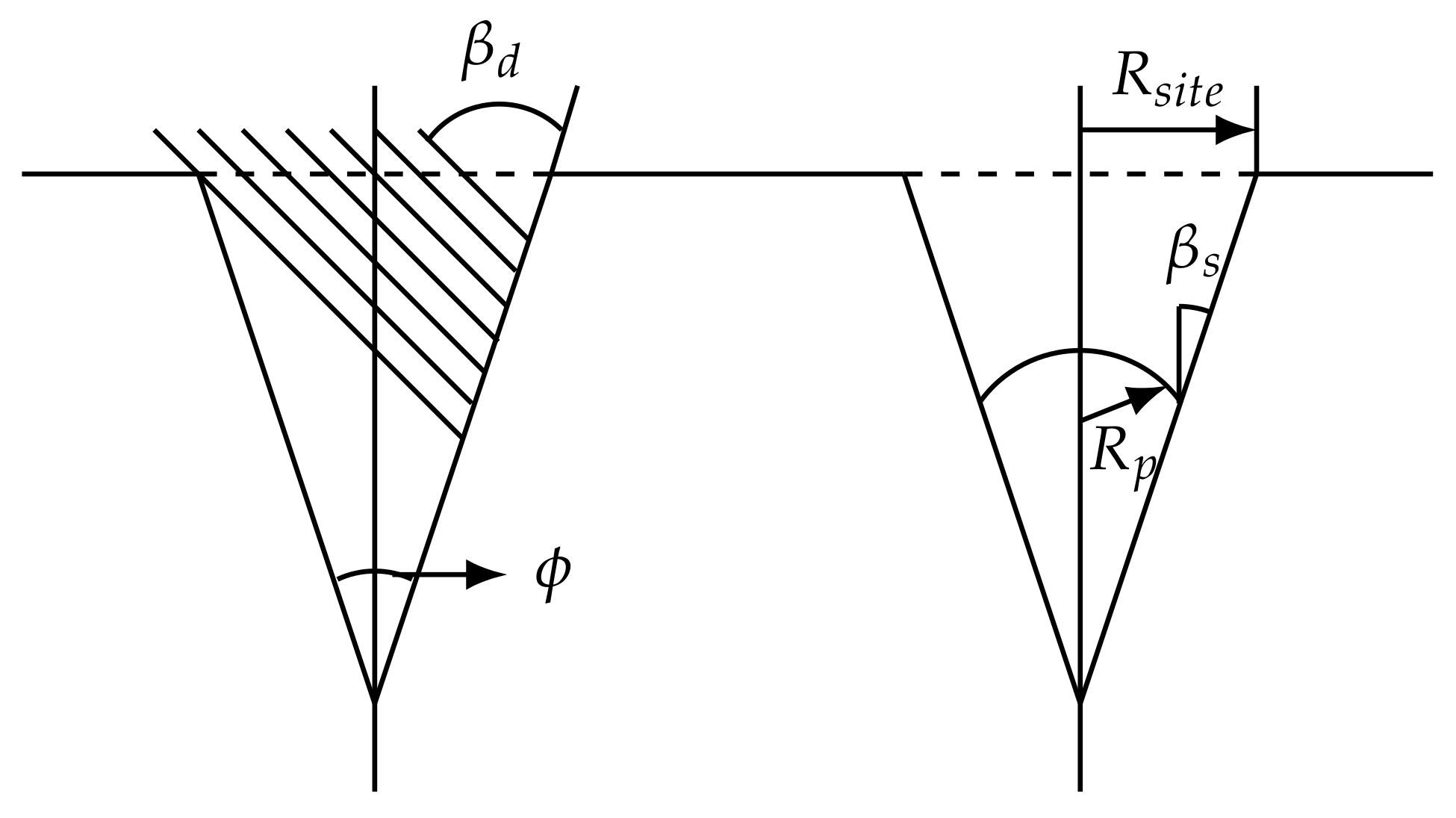
2.5.2. Initialization

Nucleation cavities present on all substrate samples have a variety of shapes and sizes. Due to the limitations on complexity on the boundary only rudimentary shapes can be set as nucleation sites. For this reason it was opted to simply represent all nucleation sites as small conical cavities due to their simple geometry and the more available literature, thus making them a good starting point on which to further expand in later works using more complex geometries (rounded sites, elongated crevices, etc.) if deemed necessary. All nucleation sites are distributed randomly across the nucleating boundary wall (see Figure 4) with a site radius ($R_{site}$) taken from a Gaussian distribution. The depth (d) is taken as a random value ($0.5R_{site}<d<1.5R_{site}$). This has been selected to represent a general surface, but to obtain an actual real surface, experimental data to correlate properties such surface roughness to the number of nucleation sites is necessary. Currently, an experimental setup is under construction (based on the work of Enríquez et al. [46]), to obtain data on the nucleation site density from real surfaces. The sites are placed in such a way that the minimum distance between each site is 1.5 times the maximum expected growth to prevent overlap of nucleating bubbles.

As was noted in the review by Jones et al. [47], only cavities containing a gas pocket are able to form bubbles in low to moderate supersaturation ratios (see Section 2.5.1, Types III and IV). For such a cavity to hold any gas, it needs to be entrapped by the moving liquid closing the cavity mouth before all of the gas has been pushed out by the moving liquid front, or alternatively to host a Type I or II nucleation event. In a study investigating this phenomena, Bankoff [48] linked the entrapment to the contact angle of the approaching liquid, noting that highly wetting liquid ($\theta \approx$ 0) will always lead to the full expulsion of any gas present in the cavity. The simple condition presented relies on the liquid’s surface tension and capability of keeping a highly rounded cap. This cap will, under the right conditions (Equation (25)), entrap gas at the bottom of a cavity with a cone angle $\varphi$.

$$2\varphi >\theta$$

(25)

This condition, however, assumes that the cavity walls are completely smooth and thus may differ from similarly sized cavities during nucleation experiments when the contact-angle of the liquid is very close to the half angle of the cavity.

A schematic representation of the entrapment process is given in Figure 5. When the DBM is initialized, the condition given by Equation (25) is used to determine whether a given cavity holds a gas pocket. This pocket is formed at the exact moment when the liquid front reaches the opposite side of the site mouth: it is thus possible to define the exact entrapped gas volume as shown by Tong et al. [49]. This gas volume $V_g$ (Equation (26)) can subsequently be used to calculate the gas pocket radius of curvature $R_p$, for the entrapped gas within the cavity (Equation (27)). An artificial bubble attached to the surface is thus generated, with a volume of gas equal to the gas pocket. The radius of the generated bubble is thus calculated from the volume assuming spherical shape and it is thus not equal to the radius of curvature. This artificial bubble serves as a place-holder for the gas pocket, basically behaving as an embryo bubble for the subsequent nucleation phase.

$$V_g=\frac{\pi R_{site}^3}{3}\frac{\sin ({\beta }_b-2\varphi ){\left[\frac{\tan \left(\varphi \right)}{\tan ({\beta }_b-\varphi )}\right]}^2}{\sin \left(\varphi \right)\sin ({\beta }_b-\varphi ){\left[1-\frac{{\tan }^2\left(\varphi \right)}{{\tan }^2({\beta }_b-\varphi )}\right]}^{2/3}}$$

(26)

$$R_p=\left[\frac{1}{\pi }\frac{3V_g}{\frac{{\cos }^3({\beta }_s-\varphi )}{\tan \left(\varphi \right)}+\left[2-3-\sin ({\beta }_s-\varphi )+{\sin }^3({\beta }_s-\varphi )\right]}\right]$$

(27)

The dynamic contact-angle ${\beta }_d$ is a property of the liquid–substrate pair, as well as the liquid–cavity contact angle of the gas embryo ${\beta }_s$. ${\beta }_d$ has been imposed equal to 90°, to avoid hydrophilicity/ hydrophobicity effects. Due to very limited data in this field, the inter cavity contact angle is difficult to be estimated for liquids which are not highly wetting. It was therefore decided to choose an average value of 30° for all liquids until more detailed information becomes available.

2.5.3. Nucleation

During each time step, all nucleation sites not currently nucleating bubbles are checked for their ability to perform nucleation. This is accomplished by firstly interpolating the dissolved gas phase concentration from the Eulerian grid to the nucleation site. Thus, a local supersaturation ratio is calculated at the centre of the nucleation site, which allows the calculation of the critical radius, as defined in Equation (24). A bubble equal to the gas pocket embryo will be created at the nucleation point if the critical radius is greater than the radius of curvature of the site, calculated through Equation (27). This bubble is artificially kept in place during the nucleation and growth, until its detachment. Any nucleation site not able to perform a nucleation event due to a local insufficient supersaturation will be skipped until the amount of dissolved gas at the nucleation site becomes large enough to enable nucleation, for instance as a consequence of local fluctuations. While the bubble is attached to the surface, it is subjected to mass transfer (as described in Section 2.2), thus growing until it is ready to detach.

2.5.4. Detachment

Bubble detachment occurs when the forces pulling the bubble upwards overcome the surface force keeping the bubble anchored to the site. Several forces play a role in this process, but research is still ongoing to describe their different effects on the detachment. In this paper, the simple approach of Fritz [50] is used: a force balance between buoyancy and surface force allows obtaining a critical radius for detachment, usually called the Fritz radius ($R_f$ in Equation (28)).

$$R_f={\left(\frac{3}{2}\frac{\sigma R_{site}}{({\rho }_l-{\rho }_g)g}\right)}^{\frac{1}{3}}$$

(28)

Upon reaching this radius, the bubble will detach and it will start rising in the column. The process of detachment is treated in the DBM as a breakup: a volume of gas equal to the cavity volume is left attached to the surface ready to nucleate a new bubble while the remaining gas is the newly formed bubble that is free to rise in the column.

2.5.5. Limitations and Assumptions

Finally, a few remarks on the limitations of the current implementation of heterogeneous bubble nucleation. The state-of-the-art detachment criterion, based on the Fritz radius, does not account for the many other relevant phenomena that might play a role. For instance, shear flow or even collisions of nucleating bubbles with neighbouring bubbles are not considered in the calculations, as well as possible coalescence with neighbouring nucleating bubbles (while they remain considered for freely rising bubbles as described in Section 2.2.1). The initialization of the nucleation sites is currently done in such a way that this will never happen, while for a real case scenario this should be included in the model. Moreover, the initial volume of the gas pocket is initialized as a spherical bubble, of which the radius is used as a detachment criterion. Compared to a conical cavity, the assumption of a spherical bubble might not result in the correct radius calculation for the detachment. In addition, our simulations now rely on fictional parameters for the nucleation sites properties (i.e., a random Gaussian distribution of site radii). However, these parameters will depend upon the surface material, the liquid properties, the gas properties, etc. These parameters need to be adjusted to obtain physical results for a real surface, which is a needed step for the required model validation.

2.5.6. Summary of the Implementation

At the DBM initialization, a surface is initialized with assigned nucleation sites, with random position, radius ($R_{site}$) taken from a Gaussian distribution and site depth (d) assigned as explained in Section 2.5.2. Equation (25) is used to check if a gas pocket is formed, of which the gas volume is calculated through Equation (26) while the pocket radius of curvature ($R_p$) is computed from Equation (27). If the local critical radius $R_c$, defined in Equation (24), is larger than the radius of curvature, an artificial bubble with equal volume as the gas pocket is generated, functioning as the bubble embryo and kept attached to the wall. These bubbles will grow, until reaching a size which allows the detachment. This size is called the Fritz radius $R_f$, as defined in Equation (28). The detachment procedure essentially follows the bubble break-up procedure; part of the bubble remains attached to the surface (representing the embryo bubble as a gas pocket in the cavity), whereas the remaining gas forms a bubble on which the body forces are computed. This bubble can then rise freely through the column.

3. Results

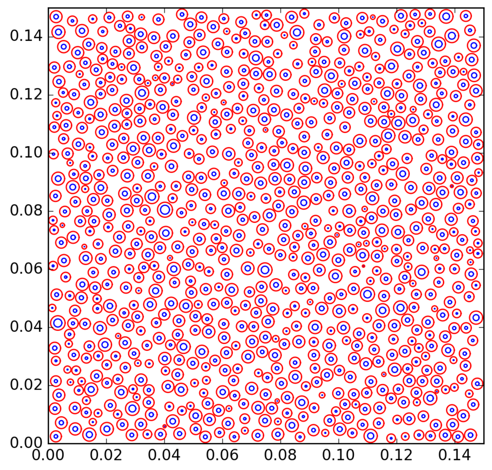
3.1. Numerical Setup

The considered domain is a square box of $15\mathrm{c}\mathrm{m}$ described by a Eulerian grid of $30\times 30\times 30$ grid nodes. The liquid is water at standard conditions (${\rho }_l=1000\mathrm{k}\mathrm{g}·{\mathrm{m}}^3$, $\sigma =0.073\mathrm{N}·\mathrm{m}$ and ${\mu }_l={10}^{-3}\mathrm{Pa}·\mathrm{s}$). The dissolved gas is CO₂, which is initially perfectly mixed in the liquid bulk with different mass fractions, corresponding to different initial supersaturation ratios. The typical time step is $1\mathrm{m}\mathrm{s}$ for both the species and the flow solvers while bubble movements are computed using time steps 20 times smaller. A total of 1300 nucleation sites is randomly generated with a size taken from a Gaussian distribution with a mean of $0.5\mathrm{m}\mathrm{m}$ and a standard deviation of $0.3\mathrm{m}\mathrm{m}$, chosen to obtain a relatively dense surface coverage. As anticipated before, this will in the future be linked with real material properties. Out of these nucleation sites, a total of 592 gas pockets are formed, as explained in the previous section.

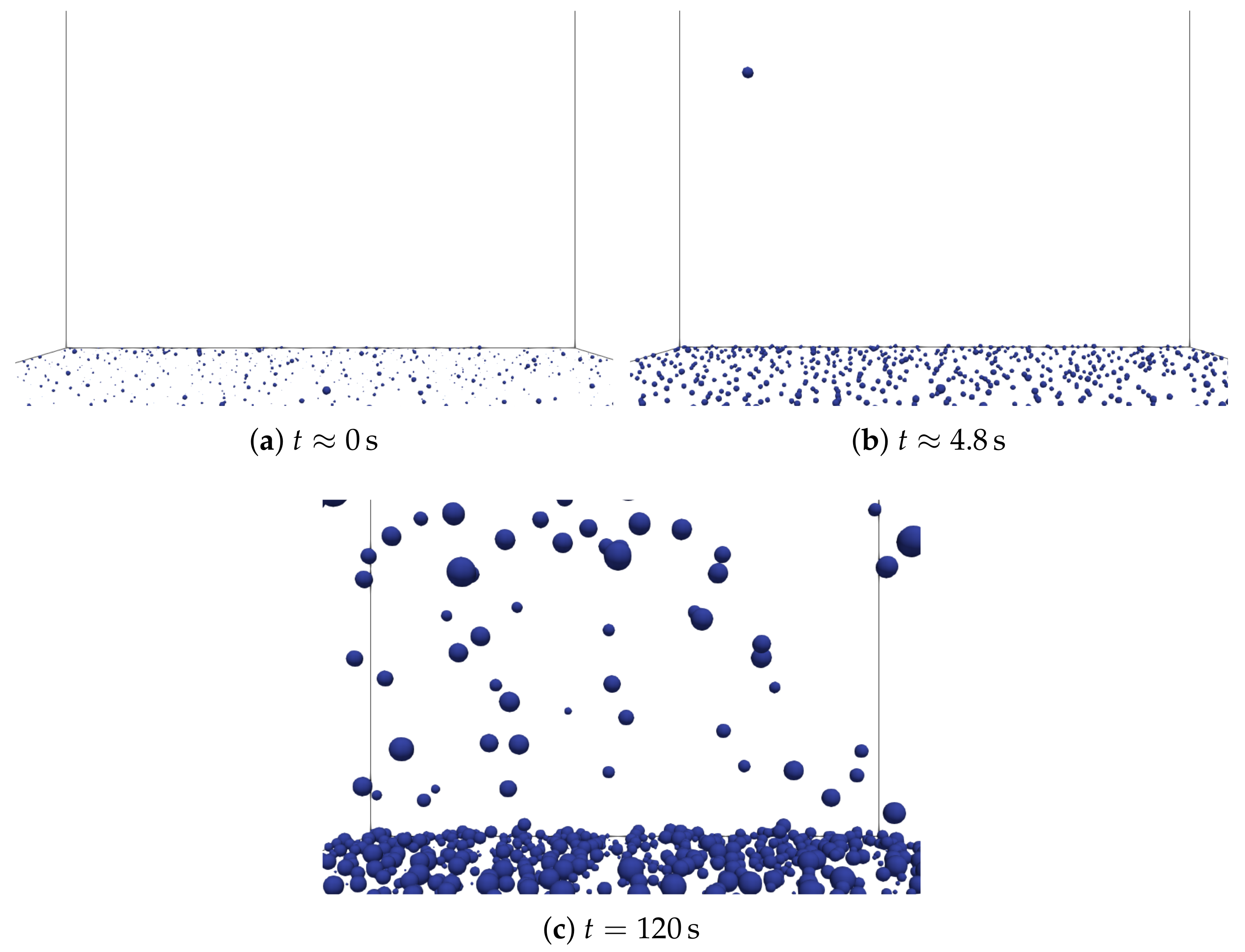
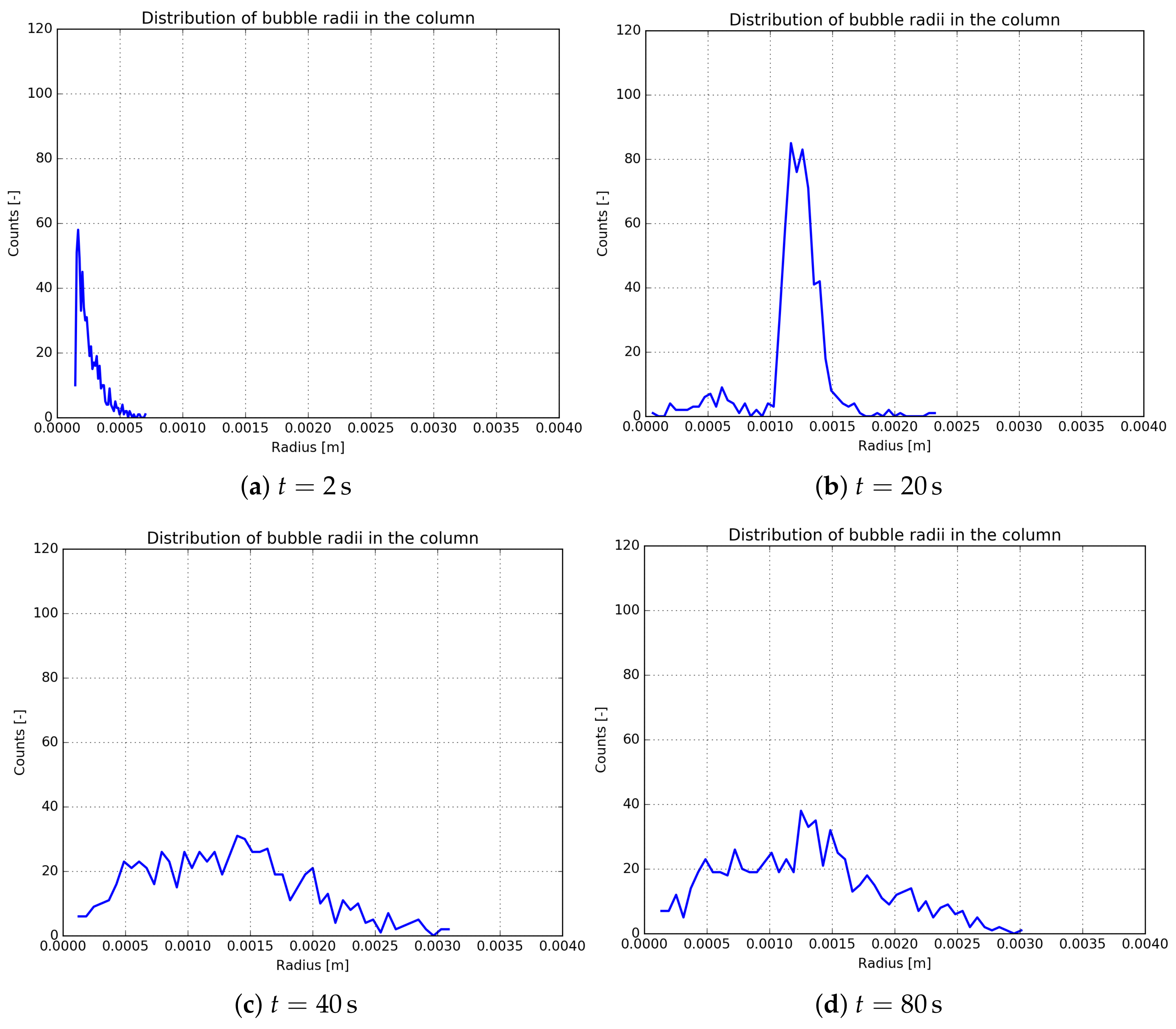
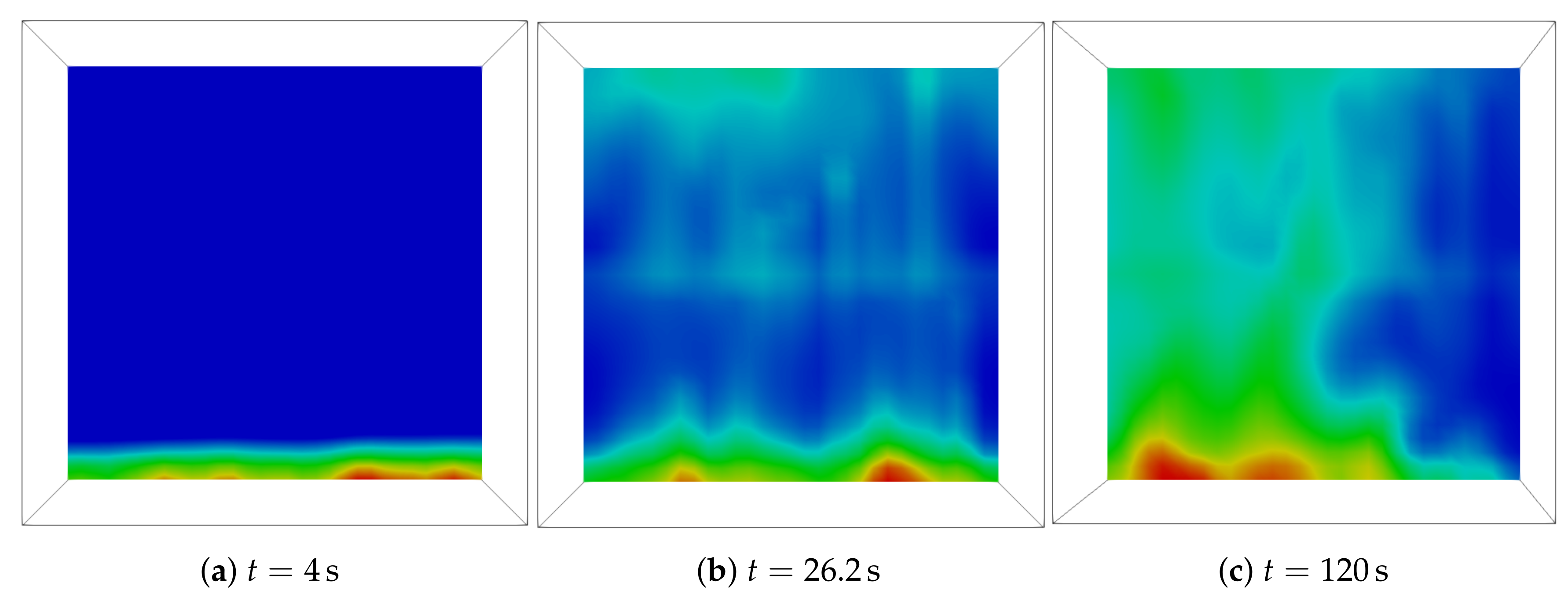
3.2. Analysis of the Nucleation Process

A snapshot of the bubble nucleation, growth and detachment is shown in Figure 6.

At the beginning, the gas pockets are represented as a bubble with equal volume attached to the surface. As a consequence of mass transfer, the pockets start growing, until the first one reaches a diameter equal to the Fritz radius and detaches, as visible in Figure 6b. After some time, most of the sites reach a pseudo-steady state in which the system is continuously forming bubbles. This pseudo-steady state, where the supersaturation in the liquid is reducing as the concentration of dissolved gas starts depleting as a consequence of the bubble formation, is also visible in terms of average bubble sizes in the column (see Figure 7).

The first peak (slowly shifting to the right) represents the gas pockets volumes, growing because of mass transfer. When the detachment of bubbles starts, the distribution tends to become wider and flatter, because of the presence of large bubbles rising in the column and small nuclei growing on the surface.

The initial growth of bubbles attached to the surface also affects the concentration profiles in the column, where the supersaturated liquid starts desaturating closer to the surface (see Figure 8a) as a consequence of the mass transfer of dissolved gas in the liquid towards the growing bubbles. Indeed, a depletion zone can be observed, which is slowly extending upwards. As soon as bubbles start detaching, this zone gets perturbed, as visible in Figure 8b. Channel-like structures of lower concentration areas represent the wake of bubbles rising, which meanwhile still grow because of mass transfer. This is a transition regime, which ends when swarms of bubbles detach steadily from the surface inducing more mixing in the system, as visible in Figure 8c.

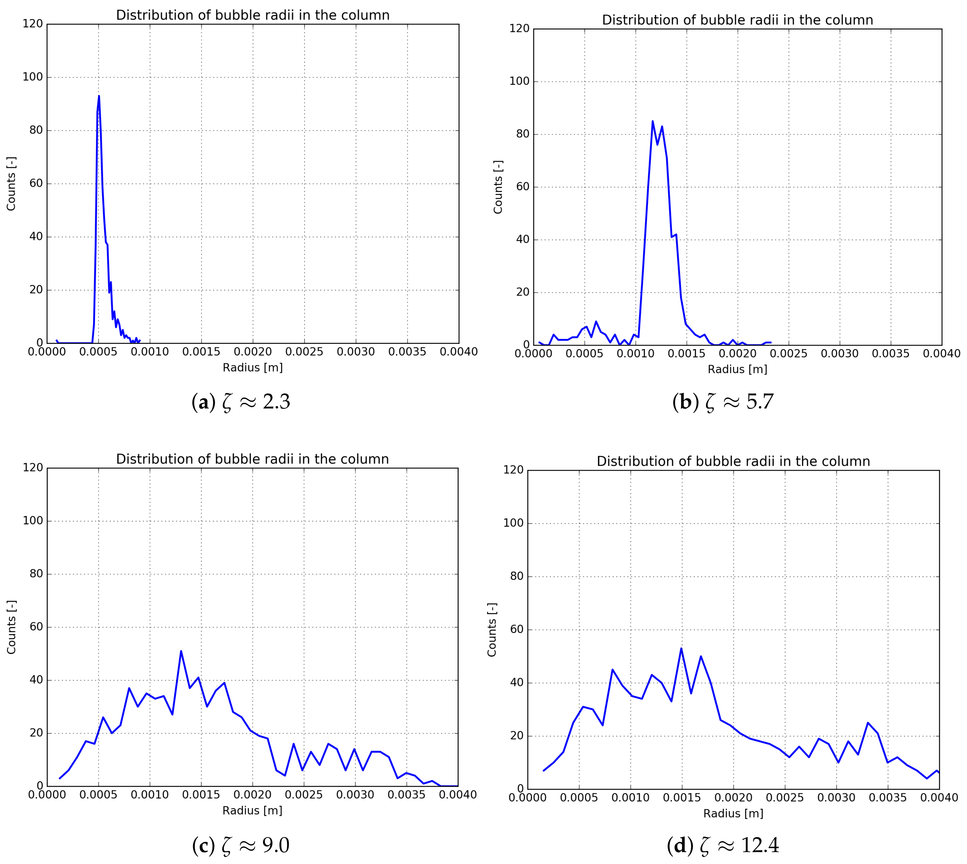
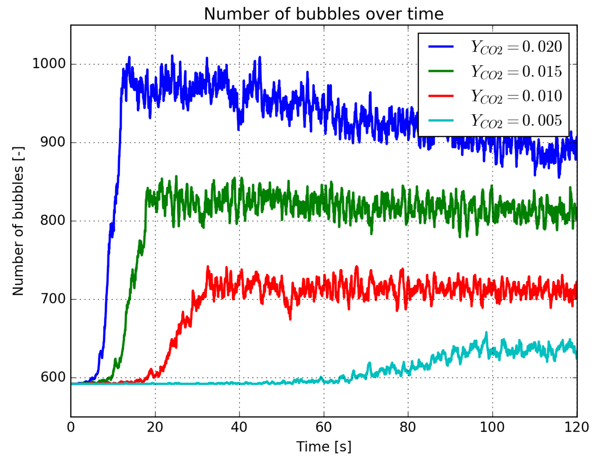
3.3. Effect of the Supersaturation Ratio

The initial supersaturation ratio has a large influence, not only because it changes the amount of gas that can be transferred to the gas phase (and thus directly the mass transfer rate), but also because it affects properties such as the critical radius (defined in Equation (24)) that controls the nucleation process. When the supersaturation is increased, bubbles grow much faster on the surface, detaching earlier. The critical radius is also smaller, which implies that more nucleation sites are active. This is clearly visible in Figure 9, showing the bubble size distributions in the column for different supersaturation ratios.

At the lowest initial supersaturation, the nucleation process is still in its early stages, corresponding to the situation where bubbles are still growing on the surface, while for larger ratios (Figure 9c,d) the surface is already bubbling and a wider bubble size distribution has been established. For the highest supersaturation ratio, the bubble size distribution has shifted slightly to larger diameters, which can be attributed to two effects: (i) bubbles grow much faster on the surface, increasing the number of large bubbles in the column compared to the number of small bubbles on the surface; and (ii) the bubbles can grow larger because of increased mass transfer and bubble coalescence (a higher bubble number density increases the bubble encounter frequency). It is worth mentioning that a time span of $20\mathrm{s}$ seems rather unrealistic for an initial supersaturation of about 2.3 to not have detached any bubble yet, but this is related to the nucleation sites density and the relatively small selected radii of the original gas pockets, requiring the bubbles to grow for a relatively long time span before the first bubble is detached. This work is the first step in the integration of a nucleation model, where in the future the model parameters will be improved with experimental data.

As bubbles detach faster, more of them will be present in the column at the same time, as can be discerned in Figure 10, showing the total number of bubbles in the column as a function of time. Indeed, the total number of bubbles in the column is much smaller for the smallest supersaturation, while at the same time it takes much more time to develop a steady rate of bubble formation. On the other hand, the depletion of concentration starts to become pronounced for the highest supersaturation, where bubbles are quickly formed, but where the number of bubbles is already decreasing, corresponding to the decrease in liquid concentration.

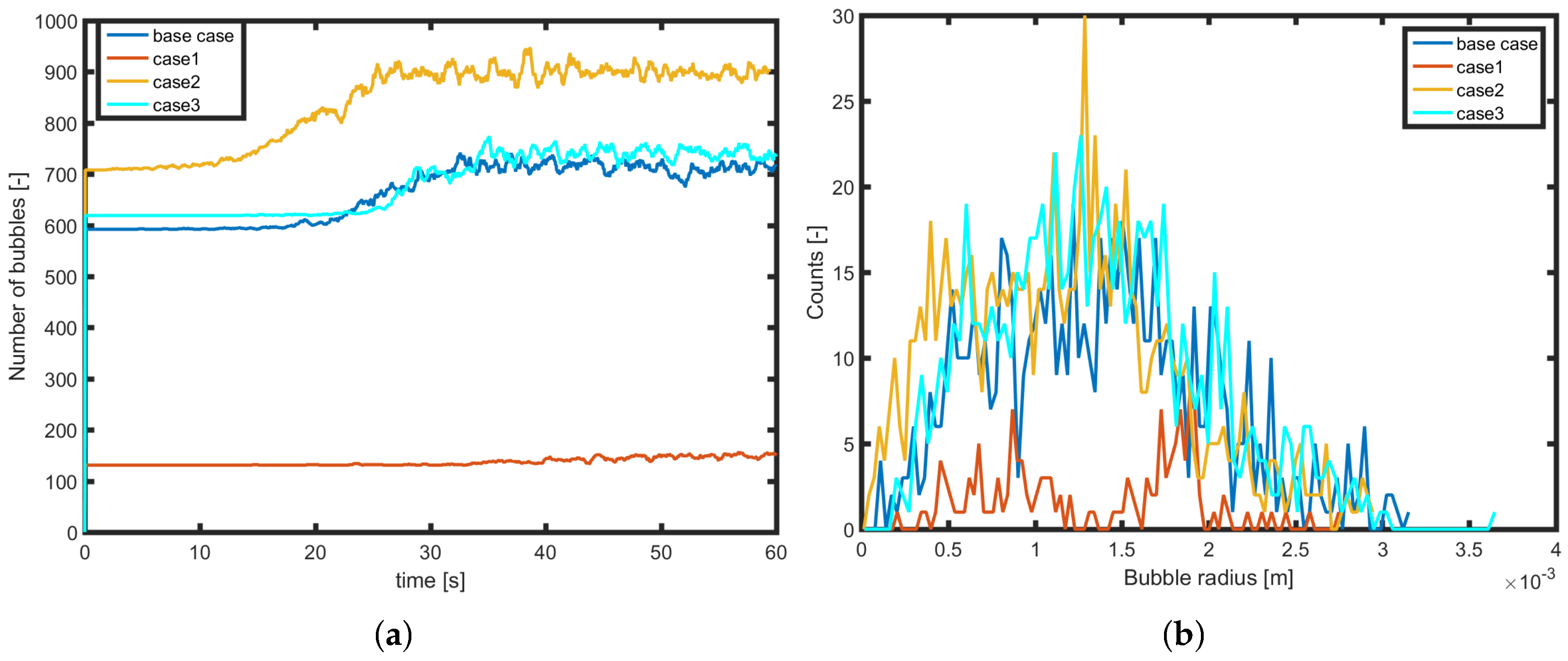
3.4. Effect of the Surface Properties

In this work, the surface nucleation properties have been randomly generated. Real surfaces may have different properties, which can be determined by dedicated measurements. To put into context how the system will respond to a certain variation in the nucleation properties, a sensitivity analysis of nucleation site parameters has been performed. The case with a starting supersaturation ratio of 5.7 (mass fraction of 0.015 of CO₂) has been taken as the base case, while in the other three the total number of sites (Case 1), the mean nucleation site radius $R_{site}$ (Case 2) or the standard deviation of the nucleation site radii distribution (Case 3) has been varied. Thus, the numerical setup is as described in Section 3.1, with a starting supersaturation of 5.7. A list of varied parameters for each case is shown in

Table 2. Description of sensitivity analysis cases.

Case	Description	Parameters
base case	$\zeta \approx 5.7$, case described in Section 3.1	N${}_{site}$ = 1300
		R${}_{mean}$ = 0.5 $\mathrm{m}\mathrm{m}$
		s = 0.3 $\mathrm{m}\mathrm{m}$
Case 1	Decreased number of nucleation sites	N${}_{site}$ = 200
Case 2	Decreased mean radius of radii distribution	R${}_{mean}$ = 0.25 $\mathrm{m}\mathrm{m}$
Case 3	Decreased standard deviation of radii distribution	s = 0.2 $\mathrm{m}\mathrm{m}$

.

In Figure 11a, it can be observed that the number of bubbles in the column is drastically reduced for Case 1, as a consequence of the lower number of nucleation sites. Indeed, out of the predefined 200 sites, a total number of 131 gas pockets is available for nucleation. This slows down the nucleation process considerably, which affects the occurrence of all bubble sizes, as seen in the bubble size distribution in Figure 11b. Indeed, since more bubbles are still growing attached to the surface, the bubble size distribution becomes more similar to the one of lower supersaturation, with a clear bimodal peak due to the presence of a considerable amount of bubbles still growing at the surface. On the other hand, the effect of the change in the standard deviation of the nucleation sites (Case 3) is not as influential, and results in a similar bubble size distribution as the base case. Unless the site radius distribution is generated with a very wide distribution, the site radius distribution is of less importance for the nucleation process.

Changing the mean radius however (Case 2) shows a considerable effect in the number of bubbles produced. The reason for this particular increase lies in the number density of nucleation sites. Indeed, when they are generated with a smaller average radius, more sites can be fitted on the surface, leading to a larger number of nucleating bubbles. The difference in size does not induce a difference in trends, which can be seen to match well with the base case and Case 3. However, it is visible that in Case 2 the detachment phase starts slightly earlier compared to the base case. This is related with the Fritz radius, which is proportional to the cube root of the nucleation site radius, allowing bubbles to detach earlier when the site has a smaller size. Although the number of bubbles changes, the bubble size distribution does not; this is because the size is dominated by bubbles rising in the column which are mostly determined in size by the degree of supersaturation, while for Case 1 the majority of bubbles are still attached to the nucleation sites.

As visible from this short sensitivity analysis, surface properties are able to influence the number of nucleated bubbles and in some cases the instantaneous bubble size distribution. For this reason, it is important to stress again the importance of dedicated measurements to perform simulations of real surfaces.

4. Conclusions and Outlook

This work has discussed the integration of heterogeneous bubble nucleation into a Discrete Bubble Model. An algorithm has been proposed and implemented to study the formation of bubbles on a solid surface as a result of supersaturation, assuming random conical nucleation sites.

A clear initial regime is visible where bubbles are slowly growing while remaining attached to the surface, with the formation of a depletion layer close to the bottom surface. As soon as bubbles start reaching the Fritz radius, and thus detach, they introduce a more vigorous mixing which breaks the depletion layer. The increase in the initial supersaturation not only decreases the time span of this first growing regime, but also increases the total number of bubbles in the system and their sizes. For higher supersaturation ratios, the total number of bubbles is clearly decreasing in time, as a consequence of the fast depletion of the dissolved gas in the system.

A sensitivity analysis of surface properties has been performed. The nucleation sites number density has a clear effect both in the number of bubbles and in the bubble size distribution. Fewer sites will form fewer bubbles and will not mix the system leading to an overall slower phase transition process. On the other hand, decreasing the average site radius will lead to a higher number of bubbles as a consequence of the changed site density, while also slightly accelerating the detachment process because of the average smaller Fritz radius.

Despite its interesting capabilities, this model is not yet complete. Firstly, other effects for detachment, for instance shear flows, have to be included. Moreover, bubble interactions between bubbles that are still attached to the surface could lead to a potential early detachment after a collision or a coalescence event between two bubbles attached to neighbouring nucleation sites, increasing the bubble formation rate. The effect of depletion should be studied further, as well as the fact that a bubble attached to the surface will experience lower mass transfer rates as a consequence of the lower available interfacial area. The latter two phenomena have been studied experimentally for single bubbles by Moreno Soto et al. [51] and Enríquez et al. [52], respectively, and could represent a relevant topic for future research at the meso-scale. In addition, experimental validation determining nucleation model parameters of actual surfaces is of extreme importance and has been started following the work of Enríquez et al. [46].

To conclude, the similarities with boiling flows have been already highlighted in literature [12]. The model here presented could be expanded to a boiling case, where similar simulations can be performed for instance at different Pr numbers.

References

1. Darmana, D.; Deen, N.G.; Kuipers, J.A.M. Detailed modeling of hydrodynamics, mass transfer and chemical reactions in a bubble column using a discrete bubble model. Chem. Eng. Sci. 2005, 60, 3383–3404. [Google Scholar] [CrossRef] [Green Version]
2. Besagni, G.; Inzoli, F.; Ziegenhein, T. Two-Phase Bubble Columns: A Comprehensive Review. ChemEngineering 2018, 2, 13. [Google Scholar] [CrossRef]
3. Van Sint Annaland, M.; Deen, N.G.; Kuipers, J.A.M. Multi-Level Modeling of Dispersed Gas-Liquid Two-Phase Flows; Springer: Berlin, Germany, 2003. [Google Scholar]
4. Volanschi, A.; Oudejans, D.; Olthuis, W.; Bergveld, P. Gas phase nucleation core electrodes for the electrolytical method of measuring the dynamic surface tension in aqueous solutions. Sens. Actuators B 1996, 35–36, 73–79. [Google Scholar] [CrossRef]
5. Verhaart, H.; de Jonge, R.; van Stralen, S. Growth rate of a gas bubble during electrolysis in supersaturated liquid. Int. J. Heat Mass Transf. 1980, 23, 293–299. [Google Scholar] [CrossRef]
6. Liger-Belair, G.; Vignes-Adler, M.; Voisin, C.; Bertrand, R.; Jeandet, P. Kinetics of Gas Discharging in a Glass of Champagne: The Role of Nucleation Sites. Langmuir 2002, 18, 1294–1301. [Google Scholar] [CrossRef]
7. Amon, M.; Denson, C.D. A study of the dynamics of foam growth: Analysis of the growth of closely spaced spherical bubbles. Polym. Eng. Sci. 1984, 24, 1026–1034. [Google Scholar] [CrossRef]
8. Pooladi-Darvish, M.; Firoozabadi, A. Solution-gas drive in heavy oil reservoirs. J. Can. Pet. Technol. 1999, 38, 54–61. [Google Scholar] [CrossRef]
9. Askari, E.; Proulx, P.; Passalacqua, A. Modelling of Bubbly Flow Using CFD-PBM Solver in OpenFOAM: Study of Local Population Balance Models and Extended Quadrature Method of Moments Applications. ChemEngineering 2018, 2, 8. [Google Scholar] [CrossRef]
10. Liu, L.; Cai, W.; Chen, Y.; Wang, Y. Fluid Dynamics and Mass Transfer Study of Electrochemical Oxidation by CFD Prediction and Experimental Validation. Ind. Eng. Chem. Res. 2018, 57, 6493–6504. [Google Scholar] [CrossRef]
11. El-Askary, W.; Sakr, I.; Ibrahim, K.; Balabel, A. Hydrodynamics characteristics of hydrogen evolution process through electrolysis: Numerical and experimental studies. Energy 2015, 90, 722–737. [Google Scholar] [CrossRef]
12. Liu, H.; Pan, L.M.; Wen, J. Numerical simulation of hydrogen bubble growth at an electrode surface. Can. J. Chem. Eng. 2015, 94, 192–199. [Google Scholar] [CrossRef]
13. Yang, Z.; Peng, X.; Ye, P. Numerical and experimental investigation of two phase flow during boiling in a coiled tube. Int. J. Heat Mass Transf. 2008, 51, 1003–1016. [Google Scholar] [CrossRef]
14. Zhuan, R.; Wang, W. Simulation on nucleate boiling in micro-channel. Int. J. Heat Mass Transf. 2010, 53, 502–512. [Google Scholar] [CrossRef]
15. Yang, Z.L.; Dinh, T.; Nourgaliev, R.; Sehgal, B. Numerical investigation of bubble coalescence characteristics under nucleate boiling condition by a lattice-Boltzmann model. Int. J. Therm. Sci. 2000, 39, 1–17. [Google Scholar] [CrossRef]
16. Weijs, J.H.; Snoeijer, J.H.; Lohse, D. Formation of Surface Nanobubbles and the Universality of Their Contact Angles: A Molecular Dynamics Approach. Phys. Rev. Lett. 2012, 108, 104501. [Google Scholar] [CrossRef] [PubMed]
17. van der Linde, P.; Moreno Soto, Á.; Peñas-López, P.; Rodríguez-Rodríguez, J.; Lohse, D.; Gardeniers, H.; van der Meer, D.; Fernández Rivas, D. Electrolysis-Driven and Pressure-Controlled Diffusive Growth of Successive Bubbles on Microstructured Surfaces. Langmuir 2017, 33, 12873–12886. [Google Scholar] [CrossRef] [PubMed]
18. Mandin, P.; Hamburger, J.; Bessou, S.; Picard, G. Modelling and calculation of the current density distribution evolution at vertical gas-evolving electrodes. Electrochim. Acta 2005, 51, 1140–1156. [Google Scholar] [CrossRef]
19. Nierhaus, T.; van Parys, H.; Dehaeck, S.; van Beeck, J.; Deconinck, H.; Deconinck, J.; Hubin, A. Simulation of the Two-Phase Flow Hydrodynamics in an IRDE Reactor. J. Electrochem. Soc. 2009, 156, P139–P148. [Google Scholar] [CrossRef]
20. Van Parys, H.; van Damme, S.; Maciel, P.; Nierhaus, T.; Tomasoni, F.; Hubin, A.; Deconinck, H.; Deconinck, J. Eulerian-Lagrangian Model for gas-evolving processes based on supersaturation. WIT Trans. Eng. Sci. 2009, 65, 109–118. [Google Scholar] [CrossRef]
21. Van Damme, S.; Maciel, P.; van Parys, H.; Deconinck, J.; Hubin, A.; Deconinck, H. Bubble nucleation algorithm for the simulation of gas evolving electrodes. Electrochem. Commun. 2010, 12, 664–667. [Google Scholar] [CrossRef]
22. Hreiz, R.; Abdelouahed, L.; Fünfschilling, D.; Lapicque, F. Electrogenerated bubbles induced convection in narrow vertical cells: PIV measurements and Euler–Lagrange CFD simulation. Chem. Eng. Sci. 2015, 134, 138–152. [Google Scholar] [CrossRef]
23. Delnoij, E.; Kuipers, J.A.M.; van Swaaij, W.P.M. A three-dimensional CFD model for gas-liquid bubble columns. Chem. Eng. Sci. 1999, 54, 2217–2226. [Google Scholar] [CrossRef]
24. Lau, Y.M.; Bai, W.; Deen, N.G.; Kuipers, J.A.M. Numerical study of bubble break-up in bubbly flows using a deterministic Euler-Lagrange framework. Chem. Eng. Sci. 2014, 108, 9–22. [Google Scholar] [CrossRef]
25. Vreman, A.W. An eddy-viscosity subgrid-scale model for turbulent shear flow: Algebraic theory and applications. Phys. Fluids 2004, 16, 3670–3681. [Google Scholar] [CrossRef]
26. Dijkhuizen, W.; Roghair, I.; Van Sint Annaland, M.; Kuipers, J.A.M. DNS of gas bubbles behaviour using an improved 3D front tracking model–Drag force on isolated bubbles and comparison with experiments. Chem. Eng. Sci. 2010, 65, 1415–1426. [Google Scholar] [CrossRef]
27. Roghair, I.; Lau, Y.M.; Deen, N.G.; Slagter, H.M.; Baltussen, M.W.; Van Sint Annaland, M.; Kuipers, J.A.M. On the drag force of bubbles in bubble swarms at intermediate and high Reynolds numbers. Chem. Eng. Sci. 2011, 66, 3204–3211. [Google Scholar] [CrossRef]
28. Tomiyama, A.; Tamai, H.; Zun, I.; Hosokawa, S. Transverse migration of single bubbles in simple shear flows. Chem. Eng. Sci. 2002, 57, 1849–1858. [Google Scholar] [CrossRef]
29. Auton, T.R. The lift force on a spherical rotational flow. J. Fluid Mech. 1987, 183, 199–218. [Google Scholar] [CrossRef]
30. Tomiyama, A.; Matsuoka, T.; Fukuda, T.; Sakaguchi, T. A Simple Numerical Method for Solving an Incompressible Two-Fluid Model in a General Curvilinear Coordinate System. In Multiphase Flow 1995; Kyoto University: Kyoto, Japan, 1995; pp. 241–252. [Google Scholar] [CrossRef]
31. Jain, D.; Deen, N.G.; Kuipers, J.A.M. Numerical modeling of carbon dioxide chemisorption in sodium hydroxide solution in a micro-structured bubble column. Chem. Eng. Sci. 2015, 137, 685–696. [Google Scholar] [CrossRef]
32. Legendre, D.; Zevenhoven, R. A numerical Euler–Lagrange method for bubble tower CO2 dissolution modeling. Chem. Eng. Res. Des. 2016, 111, 49–62. [Google Scholar] [CrossRef]
33. Asad, A.; Kratzsch, C.; Schwarze, R. Influence of drag closures and inlet conditions on bubble dynamics and flow behavior inside a bubble column. Eng. Appl. Comput. Fluid Mech. 2017, 11, 127–141. [Google Scholar] [CrossRef]
34. Mer, S.; Praud, O.; Neau, H.; Merigoux, N.; Magnaudet, J.; Roig, V. The emptying of a bottle as a test case for assessing interfacial momentum exchange models for Euler–Euler simulations of multi-scale gas-liquid flows. Int. J. Multiph. Flow 2018, 106, 109–124. [Google Scholar] [CrossRef] [Green Version]
35. Deen, N.G.; Van Sint Annaland, M.; Kuipers, J.A.M. Multi-scale modeling of dispersed gas-liquid two-phase flow. Chem. Eng. Sci. 2004, 59, 1853–1861. [Google Scholar] [CrossRef]
36. Magnaudet, J.; Eames, I. The Motion of High-Reynolds-Number Bubbles in Inhomogeneous Flows. Annu. Rev. Fluid Mech. 2000, 32, 659–708. [Google Scholar] [CrossRef]
37. Hoomans, B.P.B.; Kuipers, J.A.M.; Briels, W.J.; van Swaaij, W.P.M. Discrete particle simulation of bubble and slug formation in a two-dimensional gas-fluidised bed: A hard-sphere approach. Chem. Eng. Sci. 1996, 51, 99–118. [Google Scholar] [CrossRef] [Green Version]
38. Prince, M.J.; Blanch, H.W. Bubble coalescence and break-up in air-sparged bubble columns. AIChE J. 1990, 36, 1485–1499. [Google Scholar] [CrossRef]
39. Sommerfeld, M.; Bourloutski, E.; Bröder, D. Euler/Lagrange Calculations of Bubbly Flows with Consideration of Bubble Coalescence. Can. J. Chem. Eng. 2003, 81, 508–518. [Google Scholar] [CrossRef]
40. Liao, Y.; Lucas, D. A literature review of theoretical models for drop and bubble breakup in turbulent dispersions. Chem. Eng. Sci. 2009, 64, 3389–3406. [Google Scholar] [CrossRef]
41. Bird, R.B.; Stewart, W.E.; Lightfoot, E.N. Transport Phenomena, 2nd ed.; John Wiley & Sons: New York, NY, USA, 2007; pp. 240–241. [Google Scholar]
42. Balay, S.; Abhyankar, S.; Adams, M.F.; Brown, J.; Brune, P.; Buschelman, K.; Dalcin, L.; Eijkhout, V.; Gropp, W.D.; Kaushik, D.; et al. PETSc Users Manual; Technical Report ANL-95/11, Revision 3.7; Argonne National Laboratory: Lemont, IL, USA, 2016.
43. Balay, S.; Gropp, W.D.; McInnes, L.C.; Smith, B.F. Efficient Management of Parallelism in Object Oriented Numerical Software Libraries. In Modern Software Tools in Scientific Computing; Arge, E., Bruaset, A.M., Langtangen, H.P., Eds.; Birkhäuser Press: Basel, Switzerland, 1997; pp. 163–202. [Google Scholar]
44. Deen, N.G.; Solberg, T.; Hjertager, B.H. Large eddy simulation of the Gas-Liquid flow in a square cross-sectioned bubble column. Chem. Eng. Sci. 2001, 56, 6341–6349. [Google Scholar] [CrossRef]
45. Ogata, A.; Banks, R.B. A Solution of the Differential Equation of Longitudinal Dispersion in Porous Media; Technical Report; US Government Printing Office: Washington, DC, USA, 1961.
46. Enríquez, O.R.; Hummelink, C.; Bruggert, G.W.; Lohse, D.; Prosperetti, A.; van der Meer, D.; Sun, C. Growing bubbles in a slightly supersaturated liquid solution. Rev. Sci. Instrum. 2013, 84, 065111. [Google Scholar] [CrossRef] [PubMed] [Green Version]
47. Jones, S.F.; Evans, G.M.; Galvin, K.P. Bubble nucleation from gas cavities—A review. Adv. Colloid Interface Sci. 1999, 80, 27–50. [Google Scholar] [CrossRef]
48. Bankoff, S. Entrapment of Gas in the Spreading of a Liquid Over a Rough Surface. AIChE J. 1958, 4, 24–26. [Google Scholar] [CrossRef]
49. Tong, W.; Bar-Cohen, A.; Simons, T.; You, S. Contact angle effects on boiling incipience of highly-wetting liquids. Int. J. Heat Mass Transf. 1990, 33, 91–103. [Google Scholar] [CrossRef]
50. Fritz, W. Maximum Volume of Vapor Bubbles. Phys. Z. 1935, 36, 354–379. [Google Scholar]
51. Moreno Soto, A.; Prosperetti, A.; Lohse, D.; van der Meer, D. Gas depletion through single gas bubble diffusive growth and its effect on subsequent bubbles. J. Fluid Mech. 2017, 831, 474–490. [Google Scholar] [CrossRef] [Green Version]
52. Enríquez, O.R.; Sun, C.; Lohse, D.; Prosperetti, A.; van der Meer, D. The quasi-static growth of CO2 bubbles. J. Fluid Mech. 2014, 741. [Google Scholar] [CrossRef]
Figure 1. Schematic representation of the collision process for two bubbles of the same mass (here depicted in 2D for clarity).
Chemengineering 02 00039 g001
Figure 2. Comparison of the DBM species solver with the analytical solution for a unidirectional convection-diffusion flow, for different grid resolutions: (a) analytical vs. simulations data, where the analytical solution is represented by the black line; and (b) L2-norm relative error vs. grid elements.
Chemengineering 02 00039 g002
Figure 3. First (top line) and second (bottom line) order reactions in a batch reactor: comparison with the analytical solutions.
Chemengineering 02 00039 g003
Figure 4. Top down view of the x-y plane containing randomly distributed nucleation sites. The blue circles represent the actual size of the nucleation site, whereas the red circles represent the expected maximum growth.
Chemengineering 02 00039 g004
Figure 5. Visualized parameters for Equations (26) and (27), redrawn from Tong et al. [49].
Chemengineering 02 00039 g005
Figure 6. Snapshots of the bubble nucleation process on a surface for supersaturated water with CO2 ζ 5.7 initial supersaturation: (a) the initial gas pockets volumes; (b) first detachment event; and (c) pseudo-steady state.
Chemengineering 02 00039 g006
Figure 7. Bubble size distribution in the column for a supersaturation ratio of 5.7 .
Chemengineering 02 00039 g007
Figure 8. Concentration profiles of CO2 in the liquid phase in a plane in the middle of the column for an initial supersaturation of 5.7 . Concentration ranges from red (lower) to blue (higher). The color scale is purely indicative, and is narrowed down to show the depletion of the CO2 concentration field in each image.
Chemengineering 02 00039 g008
Figure 9. Bubble size distribution in the column for different initial supersaturation ratios at t = 20 s .
Chemengineering 02 00039 g009
Figure 10. Number of bubbles in the column over time, at different initial CO2 concentrations.
Chemengineering 02 00039 g010
Figure 11. (a) Number of bubbles in the column over time, varying surface parameters. (b) Bubble size distribution in the column at t = 40 s .
Chemengineering 02 00039 g011