Abstract
Hydrogen could be a promising source fuel, and is often considered as a clean energy carrier as it can be produced by ethanol. The use of ethanol presents several advantages, because it is a renewable feedstock, easy to transport, biodegradable, has low toxicity, contains high hydrogen content, and easy to store and handle. Reforming ethanol steam occurs at relatively lower temperatures, compared with other hydrocarbon fuels, and has been widely studied due to the high yield provided for the formation of hydrogen. A new computational fluid dynamics (CFD) simulation model of the ethanol steam reforming (ESR) has been developed in this work. The reforming system model is composed from an ethanol burner and a catalytic bed reactor. The liquid ethanol is burned inside the firebox, then the radiative heat flux from burner is transferred to the catalytic bed reactor for transforming the ethanol steam mixture to hydrogen and carbon dioxide. The proposed computational model is composed of two phases—Simulation of ethanol burner by using Fire Dynamics Simulator software (FDS) (version 5.0) and a multi-physics simulation of the steam reforming process occurring inside the reformer. COMSOL multi-physics software (version 4.3b) has been applied in this work. It solves simultaneously the fluid flow, heat transfer, diffusion with chemical reaction kinetics equations, and structural analysis. It is shown that the heat release rate produced by the ethanol burner, can provide the necessary heat flux required for maintaining the reforming process. It has been found out that the mass fractions of the hydrogen and carbon dioxide mass fraction are increased along the reformer axis. The hydrogen mass fraction increases with enhancing the radiation heat flux. It was shown that Von Mises stresses increases with heat fluxes. Safety issues concerning the structural integrity of the steel jacket are also addressed. This work clearly shows that by using ethanol which has low temperature conversion, the decrease in structural strength of the steel tube is low. The numerical results clearly indicate that under normal conditions of the ethanol reforming (The temperature of the steel is about 600 °C or 1112 °F), the rupture time of the HK-40 steel alloy increases considerably. For this case the rupture time is greater than 100,000 h (more than 11.4 years).
Keywords:
ethanol burner; ethanol steam reformer; catalytic bed reactor; hydrogen production; fuel cell; CFD; Fire Dynamic Simulation software (FDS); Large Eddy Simulation (LES); radiative heat flux; convective heat flux; Multi-physics Simulation; Darcy Flow Equation; chemical kinetics; arrhenius coefficients; diffusion equation; heat transfer; thermal expansion; structural analysis; steel tube; HK-40 alloy; ultimate tensile strength; rupture time 1. Introduction
In recent decades, there has been a continuous effort to reduce global environmental pollution and fossil oil consumption [1]. According to Akande et al. [2] the demand for hydrogen has increased recently due to progress in fuel cell technologies. Fuel cells are electrochemical devices described as continuously operating batteries and are considered as a clean source of electric energy, containing high energy efficiency, and its resulting emission is just water [3]. It can be produced from different kinds of renewable feedstocks, such as ethanol. The use of ethanol as a raw material presents several advantages because it is easy to transport, biodegradable, has low toxicity, contains high hydrogen content, and easy to store and handle [4]. Furthermore, ethanol is economically, environmentally and strategically attractive as an energy source. Ethanol can be a hydrogen source for countries that lack fossil fuel resources, but have significant agricultural economy. This is feasible, because virtually any biomass can now be converted into ethanol as a result of recent advances in biotechnology [5]. These attributes have made H2 obtained from ethanol reforming a very good energy vector, especially in fuel cells applications. Hydrogen production from ethanol has advantages compared to other H2 production techniques, including steam reforming of methanol and hydrocarbons. Unlike hydrocarbons, ethanol is easier to reform and is also free of sulfur, which is a catalyst poison in the reforming of hydrocarbons [6]. Also, unlike methanol, which is produced from hydrocarbons and has a relatively high toxicity, ethanol is completely biomass-based and has low toxicity and as such it provides less risk to the population [7]. The fact that methanol is derived from fossil fuel resources also renders it an unreliable energy source in the long run. Conclusively, amongst the various processes and primary fuels that have been proposed for hydrogen production in fuel cell applications, steam reforming of ethanol is very attractive. Ethanol steam reforming (ESR) proceeds at temperatures in the range of 300–600 °C, which is significantly lower than those required for CH4 or gasoline reforming. This is an important consideration for the improved heat integration of fuel cell vehicles.
The main objective of the computational fluid dynamics (CFD) modeling in this work is to analyze the structural integrity and performance of an industrial ESR system with considerable modeling accuracy that can help evaluate various modeling assumptions usually employed.
Extensive work has been performed on the mathematical modeling the development of first-principles reformer models. With the dramatic increase of computing power, CFD modeling has become an increasingly important platform for reformer modeling and design, combining physical and chemical models with detailed representation of the reformer geometry. When compared with first-principles modeling, CFD is a modeling technique with powerful visualization and computational capabilities to deal with various geometry characteristics, transport equations and boundary conditions.
A 3D CFD simulation pioneering study of the ESR in microreactors with square channels has been carried out by Uriz et al. [8]. A phenomenological kinetic model based on simple power-law rate equations and considering the following reactions—ethanol dehydrogenation to acetaldehyde, acetaldehyde steam reforming to H2 and CO2, ethanol decomposition to CO, CH4 and H2, and the water-gas shift—describes satisfactorily the ESR over a Co3O4-ZnO catalyst. The CFD computational study shows that high reforming temperatures (above 625 °C) should be avoided. This is because the decomposition of ethanol competes effectively with the dehydrogenation of the alcohol to acetaldehyde, which is the key intermediate of the ESR process, and results in a reduced hydrogen yield and an increased content of CO in the reformate stream. Their work shows that micro reactors can help to overcome these difficulties by increasing the surface area-to-volume ratio and the catalyst loading. By using these micro reactors, the operating temperature can be reduced while increasing the selectivity and maintaining the level of ethanol conversion [8].
Uriz et al. [9] showed that CFD is a very useful tool for advancing in the development and optimization of these technologies. The interest of CFD for assisting in the understanding of the behavior of hydrogen technologies is also important. Nevertheless, there are also limitations regarding the description of chemical transformations and the physics of some complex phenomena such as in multi-physics systems.
Lao et al. [10] developed a CFD model of an industrial scale steam methane reforming reactor (reforming tube) used to produce hydrogen. The CFD model of an industrial-scale reforming tube has been developed in ANSYS Fluent (version 15.0) with realistic geometry characteristics to simulate the transport and chemical reaction phenomena with approximate representation of the catalyst packing.
In this work a CFD simulation study of the ESR system has been performed. The proposed computational work is composed of two phases—simulation of ethanol burner by using fire dynamics simulator (FDS) software and a multiphysics simulation of steam reforming process occurring inside the reformer. COMSOL multi-physics software has been applied in this work. It solved simultaneously the fluid flow, heat transfer, diffusion with chemical reaction kinetics equations and structural analysis. It is probably the first time that FDS software has been applied in order to simulate the combustion processes of the burner inside the gas heated heat exchange reformer (GHHR). The FDS software is described in detail in Section 2.1 and Section 2.2. The multiphysics reformer model is described in Section 2.3. As far as I know, this work is the first coupled CFD and structural analysis study on the ESR system. The structural analysis of the reformer steel tube is essential in order to verify that the structural integrity of the tube under the operating conditions of the reformer is maintained. Steel tube rupture and cracks may cause release of the hydrogen gas to the reformer facility. Hydrogen has wide flammability limits and very low ignition energy [11]. Therefore, hydrogen present safety concerns at limited ventilation conditions because of the danger of explosive mixture formation that may cause severe damage [12,13,14]. Diéguez et al. [12] showed examples of application of CFD to safety issues such as hydrogen leakages, hydrogen flames, detonation and application of the simulation results to evaluate possible physiological injuries. They performed a CFD for simulating the Hydrogen leakage.
1.1. Mechanism of Steam Ethanol Reforming Process
The main reactions that occur during the ESR process on Ni catalyst are [15]:
• Ethanol steam reforming:
C2H5OH + 3H2O → 2CO2 + 6H2
• Ethanol decomposition to methane:
C2H5OH → CO + H2 + CH4
• Ethanol dehydration:
C2H5OH → C2H4 + H2O
• Ethanol dehydrogenation:
C2H5OH → CH3CHO + H2
• Ethanol decomposition to acetone:
2C2H5OH → CH3COCH3 + CO + 3H2
• Water-gas shift reaction:
CO + H2O → CO2 + H2
1.2. Ethanol Burner Steam Reformer
The reforming system described in this work is composed from ethanol burner and a catalytic bed reactor. The liquid ethanol is burned inside the firebox. The heat from the flue gases is transferred to the catalytic bed reactor (the theoretical model of the reformer is described in Section 2.3) for transforming the ethanol steam mixture to hydrogen and carbon dioxide. The catalyst is made from Ni/Al2O3. The schematic of the system is described in [16].
Burner Heat Transfer
The heat produced from ethanol burning from the combustion products is transferred to catalytic bed walls in by three modes (see Figure 1):
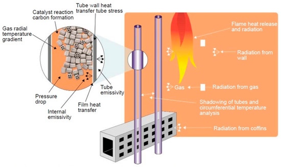
Figure 1.
Heat transfer mechanisms in steam reformer [17].
- (1)
- Convection
- (2)
- Radiation
- (3)
- Conduction
1.2.2 Convection
Heat is transferred through fluids in motion and between a fluid and solid surface in relative motion. When the motion is produced by forces other than gravity, the term forced convection is used. In engines the fluid motions are turbulent. Heat is transferred by forced convection between the in-cylinder gases and the cylinder head, valves, cylinder walls, and piston during induction, compression, expansion and exhaust processes [18].
1.2.3 Radiative Heat Transfer
There are two sources of radiative heat transfer within the burner: The high temperature burned gases and the soot particles in the ethanol flames. In the burner, most if the fuel burns in turbulent diffusion flame as fuel and air mix together. The flame is highly luminous, and soot particles are formed at an intermediate step in the combustion process [18].
1.2.4 Conduction Heat Transfer
Heat is transferred by molecular motion, through solids and through fluids at rest, due to temperature gradient. It is transferred by conduction through the reformer walls [18].
2. Materials and Methods
2.1. Fire Dynamic Simulation Modeling of the Burner
The FDS has been developed at the Building and Fire Research Laboratory (BFRL) at the National Institutes of Standards and Technology (NIST), e.g., McGrattan et al. [19,20]. This software calculates simultaneously the temperature, density, pressure, velocity, and chemical composition within each numerical grid cell at each discrete time step. It also calculates the temperature, heat flux, and mass loss rate of the enclosed solid surfaces. The latter is used in the case where the fire heat release rate is unknown. The major components of this software are:
Hydrodynamic Model—FDS code is formulated based on CFD of fire-driven fluid flow. The FDS numerical solution can be carried out using either a Direct Numerical Simulation (DNS) method or Large Eddy Simulation (LES). The latter is relatively low Reynolds numbers and is not severely limited in grid size and time step as the DNS method. In addition to the classical conservation equations considered in FDS, including mass species momentum and energy, thermodynamics-based state equation of a perfect gas is adopted along with chemical combustion reaction for a library of different fuel sources.
Combustion Model—For most applications, FDS uses a mixture fraction combustion model. The mixture fraction is a conserved scalar quantity that is defined as the fraction of gas at a given point in the flow field that originated as fuel. The model assumes that combustion is mixing controlled, and that the reaction of fuel and oxygen is infinitely fast. The mass fractions of all of the major reactants and products can be derived from the mixture fraction by means of “state relations”, empirical expressions arrived at by a combination of simplified analysis and measurement [21].
Radiation Transport—Radiative heat transfer is included in the model via the solution of the radiation transport equation for a non-scattering gray gas. In a limited number of cases, a wide band model can be used in place of the gray gas model. The radiation equation is solved using a technique similar to a finite volume method for convective transport, thus the name given to it is the Finite Volume Method (FVM) [19]. FDS also has a visual post-processing image simulation program named “smoke-view”.
2.2. Governing Equations of FDS Software
This section introduces the basic conservation equations for mass, momentum and energy for a Newtonian fluid. These are the same equations that can be found in almost any textbook on fluid dynamics or CFD.
2.2.1. Mass and Species Transport
Mass conservation can be expressed either in terms of the density, [19]:
where is the density (kg/m3), and is the velocity field (m/s). In terms of the individual gaseous specie, :
is the diffusion coefficient of component of the mixture (m2/s).
2.2.2. Momentum Transport
The momentum equation in conservative form is written [19]:
where is the force term (Pa/m). The stress tensor, (Pa), is defined [19]:
The term Sij is the symmetric rate-of-strain tensor, written using conventional tensor notation. The symbol μ is the dynamic viscosity of the fluid. The overall computation can either be treated as a DNS, in which the dissipative terms are computed directly, or as a LES, in which the large-scale eddies are computed directly and the subgrid-scale dissipative processes are modeled. The numerical algorithm is designed so that LES becomes DNS as the grid is refined. Most applications of FDS are LES. For example, in simulating the flow of smoke through a large, multi-room enclosure, it is not possible to resolve the combustion and transport processes directly. However, for small-scale combustion experiments, it is possible to compute the transport and combustion processes directly.
2.2.3. LES
The most distinguishing feature of any CFD model is its treatment of turbulence. Of the three main techniques of simulating turbulence, FDS contains only LES and DNS. There is no Reynolds-averaged Navier-Stokes (RANS) capability in FDS. LES is a technique used to model the dissipative processes (viscosity, thermal conductivity, material diffusivity) that occur at length scales smaller than those that are explicitly resolved on the numerical grid. This means that the parameters μ, k and D in the equations above cannot be used directly in most practical simulations. They must be replaced by surrogate expressions that “model” their impact on the approximate form of the governing equations. This section contains a simple explanation of how these terms are modeled in FDS. There is a small term in the energy equation known as the dissipation rate, (Pa/s) the rate at which kinetic energy is converted to thermal energy by viscosity [19]:
Following the analysis of Smagorinsky, the viscosity μ is modeled:
where Cs is an empirical constant and is a length on the order of the size of a grid cell. The bar above the various quantities denotes that these are the resolved values, meaning that they are computed from the numerical solution sampled on a coarse grid (relative to DNS). The other diffusive parameters, the thermal conductivity and material diffusivity, are related to the turbulent viscosity by [16]:
The turbulent Prandtl number and the turbulent Schmidt number are assumed to be constant for a given scenario. The model for the viscosity, , serves two roles: Firstly, it provides a stabilizing effect in the numerical algorithm, damping out numerical instabilities as they arise in the flow field, especially where vorticity is generated. Second, it has the appropriate mathematical form to describe the dissipation of kinetic energy from the flow.
2.2.4. Energy Transport
The energy conservation equation is written in terms of the sensible enthalpy, (J/kg) [19]:
The sensible enthalpy (J/kg) is a function of the temperature [19]:
where sensible heat of each component in the mixture is calculated by:
where is the HRR per unit volume from a chemical reaction (W/m3), is the energy transferred to the evaporating liquid (W/m3) and represents the conductive and radiative heat fluxes (W/m2):
2.2.5. Equation of State
The pressure is calculated by using the ideal gas equation of state (the burning occurs at atmospheric pressure which is much less than the critical pressure of the air):
where p is the pressure in (Pa), T is the temperature in (K), is the universal gas constant and is the molecular mass of the gaseous mixture in (J/mol).
2.2.6. FDS Modelling of the Ethanol Burner
The geometry of the ethanol burner model is shown in Figure 2.

Figure 2.
The geometry of the ethanol burner.
At the bottom of the burner, ethanol is injected and ignited. The ethanol burning in still air is controlled by buoyancy (see Figure 3) [22].
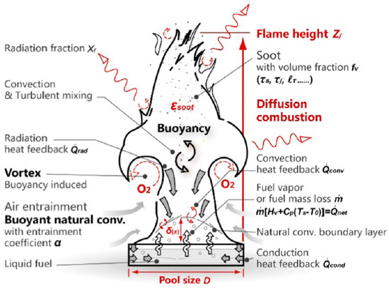
Figure 3.
The physics of liquid fuel burning [22].
It was assumed that the heat of combustion of ethanol is 26,780 (kJ/kg) [23]. The thermal conductivity of the liquid ethanol is 0.17 (W/(m·K)). The specific heat of the liquid ethanol is 2.45 (kJ/(kg·K)) and its density is 787 (kg/m3) [24]. There are three reasons that lead to justify this assumption:
- (1)
- The thermal diffusivity of the ethanol is low (the ratio between the thermal conductivity and the heat capacity multiplied by the density). Therefore, the heat front penetrates within a short distance inside the ethanol pool.
- (2)
- The radiative heat flux is attenuated inside the liquid phase.
- (3)
- The internal flow inside the liquid can be neglected (natural convection). Therefore, the convective heat transfer inside the ethanol liquid pool can be neglected.
The FDS simulation is based on the lower heating values of the ethanol. This model is flexible. There is an option to increase the heat release rate (HRR) by using fuel with higher heating value (such as gasoline or diesel).
2.3. Multiphysics Analysis of the Reformer Model
The second part deals with numerical analysis of the reformer. Figure 4 shows the geometry of this system.
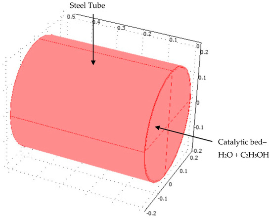
Figure 4.
3D plot of the reformer.
The reformer is made of catalyst bed material and steel tube. It has been assumed that the radius of the reformer is 0.2 m. The height of the reformer is 0.5 m. The thickness of the steel (HK-40 alloy) tube is 0.01 m (10 mm). The reformation chemical reactions occur in a porous catalytic bed where the heat is supplied through the ethanol burner to drive the endothermal reaction system. The reactor is enclosed with steel tube. Ethanol and steam are mixed in stoichiometric amounts and enter through the inlet of the catalytic reactor. COMSOL multi-physics software (version 4.3b) has been applied in this work. It solved simultaneously the fluid flow, heat transfer, diffusion with chemical reaction kinetics equations and structural analysis.
2.3.1. Model Kinetics—Reformer Bed
Inside the reformer, steam and ethanol react to form hydrogen and carbon dioxide:
The rate constant of the ESR reaction is temperature dependent according to [8]:
where A (frequency factor) is 7 × 10⁵ (1/s) and E (activation energy) is 65.8 (kJ/mol) [15].
2.3.2. Fluid Flow—Reformer Bed
The flow of gaseous species through the reformer bed is described by Darcy’s Law:
Here, denotes the gas density (kg/m3), is the viscosity (Pa·s) and is the permeability of the porous medium (m2) and is the pressure inside the reformer bed (Pa). All other boundaries are impervious, corresponding to the condition:
2.3.3. Energy Transport—Reformer Bed
The energy transport equation is used to describe the average temperature distribution in the porous bed:
The volumetric heat capacity of the bed is given by:
In the above equations, the indices “f” and “s” denote fluid and solid phases, respectively, and ε is the volume fraction of the fluid phase. Furthermore, is the temperature (K) and is the thermal conductivity of the reformer bed w/(m·K). Q represents a thermal source (w/m3), and u is the fluid velocity field (m/s). Assuming that the porous medium is homogeneous and isotropic, the steady-state equation becomes:
The volumetric heat source due to the reaction is calculated:
where r represents the reaction rate. The steam reformation of ethanol is endothermic, with an enthalpy of reaction of . Equation (19) also accounts for the conductive heat transfer in the steel tube. As no reactions occur in this domain, the description reduces to:
where is the thermal conductivity of the steel. The temperature of the gas is 700 K at the inlet. At the outlet, it is assumed that convective heat transport is dominant:
The thermal properties of the reformer are presented at Table 1 [9].

Table 1.
Thermal properties of the reformer [10].
2.3.4. Mass Transport—Reformer Bed
The mass-balance equations for the model are the Maxwell-Stefan diffusion and convection equations at steady state:
Here denotes the density (kg/m3), is the mass fraction of species i, is the molar fraction of species j, is ij component of the multicomponent Fick diffusivity (m2/s), denotes the generalized thermal diffusion coefficient (kg/(m·s)), T is the temperature (K), and is the reaction rate (kg/(m3·s)).
2.3.5. Calculation of the Binary Diffusion Coefficients—Reformer Bed
The diffusion coefficients of the components in the mixture, are obtained from the Chapman-Enskog theory [25]:
In which and are the Lennard-Jones collision diameter and collision integral between one molecule of i and one molecule of j respectively. The collision diameter is obtained from and is taken from [26]:
In which is the dimensionless temperature, where k is Boltzmann constant and is the maximum attractive energy between one molecule of i and one molecule of k. The values of and for the substances used in this work are given in Table 2 [27].
Table 2.
Properties of the gaseous species [27].
The diffusion coefficients as a function of the temperature are shown in Figure 5.
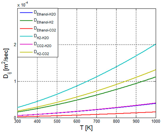
Figure 5.
The binary diffusion coefficients of the main species as a function of the temperature.
This figure clearly shows that the spreading (diffusion) gaseous species inside the reformer increases with the temperature.
2.3.6. Structural Analysis—Reformer Bed and Steel Tube
It was assumed that the tube is made of Steel HK-40. HK alloy, known as HK 40, is an austenitic Fe-Cr-Ni alloy that has been a standard heat resistant material. With moderately high temperature strength, oxidation resistance, the alloy is used in a wide variety of industrial applications such as: Ammonia, methanol and hydrogen reformers; ethylene pyrolysis coils and fittings; steam super heater tubes and fittings [28]. The thermo-physical and thermomechanical properties of the steel are listed in Table 3 [10,29].
Table 3.
Thermo-physical and thermomechanical properties of steel HK-40 [10,27].
3. Results
This section divided into two parts. In Section 3.1 the thermal results of Fire Dynamics Simulation (FDS) software are shown. In Section 3.2 the COMSOL multi-physics results for the reformer are presented.
3.1. Fire Dynamics Simulator Software Results
One advantage of FDS simulation is that it can provide much detailed information on the ethanol burner, including the local and transient gas velocity, gas temperature, species concentration, solid wall temperature, fuel burning rate, radiative heat flux, convective heat flux and HRR. The temperature field at t = 77.5 s is shown in Figure 6.
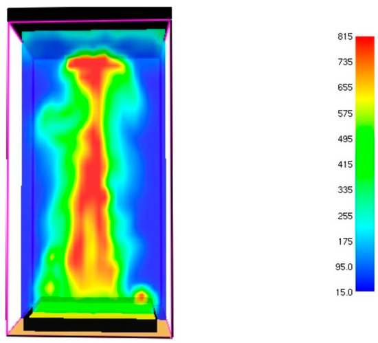
Figure 6.
Temperature field (°C) inside the burner at t = 77.5 s.
The maximal temperature at t = 77.5 s approaches to 815 °C. The velocity field of flue gases is shown in Figure 7.
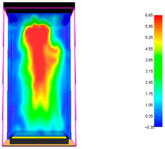
Figure 7.
Velocity field (m/s) of the flue gases at t = 77.5 s.
Figure 8 shows the radiation heat flux emitted by the burner.
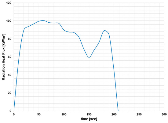
Figure 8.
Radiation heat flux produced by the ethanol burner.
Figure 8 shows that the maximal radiation heat flux is 100,000 (W/m2). It should be noted that the FDS simulation is based on the lower heating values of the ethanol. This model is flexible. There is an option to increase the HRR by using fuel with higher heating value (such as gasoline or diesel). As we shall see later, the HHR produced by the ethanol burner, can provide the necessary heat flux required for maintaining the reforming process.
3.2. Multi-Physics Analysis of the Operation of the Ethanol Steam Reformer
A parametric study has been performed in order to analyze the influence of the heat flux on the reformer performance and its structural integrity. The numerical results for heat flux of 95,300 (W/m2) are presented in Section 3.2.1. The numerical results for heat flux of 200,000 (W/m2) are presented in Section 3.2.2.
3.2.1. Multiphysics Results for Low Heat Flux Input
Figure 9 shows the 3D temperature field inside the reformer.
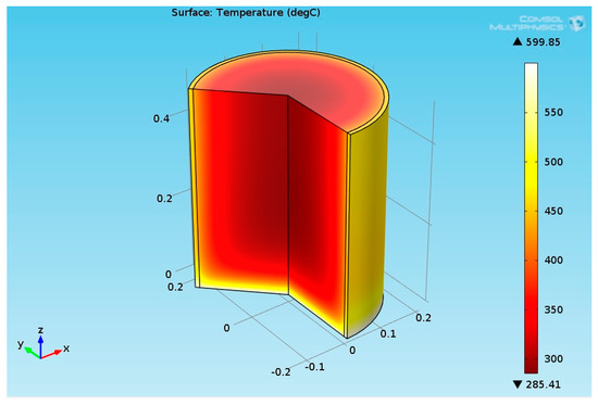
Figure 9.
3D plot of the reformer temperature field.
As can be seen from Figure 9, the temperature at the bottom section of reformer is lower than the temperature at the upper side. The temperature of the steel is much higher than the temperature of the catalyst. This is because of two reasons: Firstly, the endothermic reactions absorb the heat, and secondly, the catalyst is much thicker than the steel tube. Figure 10 shows the mass fractions of the species (ethanol, CO2 and H2O) along the reformer axis for inlet temperature of 600 °C.
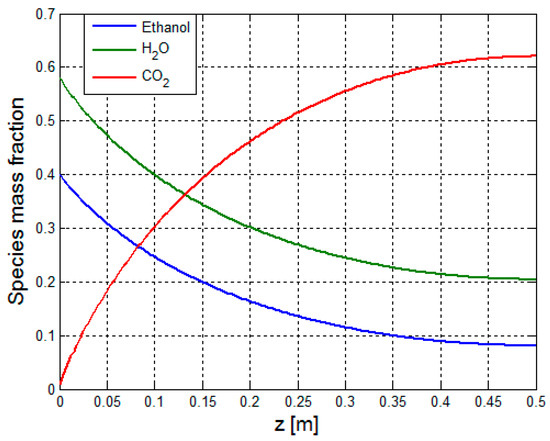
Figure 10.
Mass fractions of the species (ethanol, CO2 and H2O) along the reformer axis.
The mass fractions of the ethanol and steam decay along the reformer axis. The ethanol conversion is 80.3%. The ethanol and the steam decays at the same slope, and according to Equation (13) the amounts of ethanol and the steam are proportional to each other. Similar values have been reported in Reference [4]. From this figure it can be seen that the HRR produced by the ethanol burner, can provide the required heat flux for maintaining the reforming process. Figure 11 shows the mass fractions of the ethanol along the reformer axis for inlet temperatures of 400 °C, 500 °C and 600 °C.
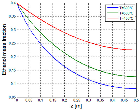
Figure 11.
Mass fractions of the ethanol along the reformer axis for various inlet temperatures.
From this figure it can be seen that for inlet temperature of 500 °C, the ethanol conversion is 70.0%. For inlet temperature of 400 °C, the ethanol conversion is 43.8%. Thus, the ethanol conversion increases with the inlet temperature. Figure 12 shows the mass fractions of hydrogen along the reformer axis.
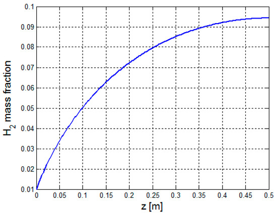
Figure 12.
Mass fractions of the H2 along reformer axis.
This figure clearly shows a considerable increasing of hydrogen mass fraction along the reformer axis. The increase in Hydrogen mass fraction is 89.4%. The sum of hydrogen, ethanol, carbon dioxide, and steam mass fraction at the reformer output is 1 as expected according the mass conservation law. The 3D Von-Mises stress distribution of reformer is shown in Figure 13.
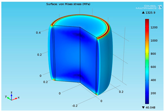
Figure 13.
3D plot of the reformer Von-Mises stress field.
As expected, the maximal stress is located at the reformer head corner. The Von-Mises thermal stresses which is developed inside the steel are much higher than the Von-Mises stresses which are developed inside the catalyst material. This is because the temperatures inside the catalyst material are much lower than the temperature in the steel tube (Since the reforming reaction is endothermic, it absorbs more heat and cools of the reformer material). According to this figure, the maximal stress in the steel tube reached to maximal value of 1.3 GPa.
3.2.2. Multiphysics Results for High Heat Flux Input
The numerical results for heat flux of 200,000 (W/m2) are presented in this section. Figure 14 shows the 3D temperature field inside the reformer.
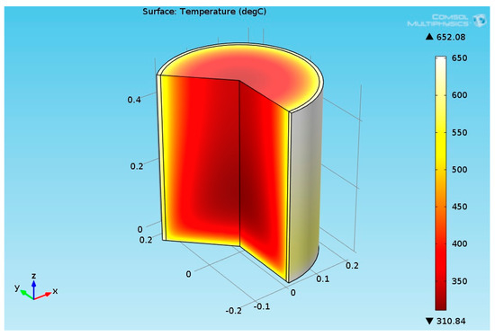
Figure 14.
3D plot of the reformer temperature field.
The maximal temperature obtained in the steel jacket for the case of 200,000 (W/m2) is about 652 °C. Figure 15 shows the mass fractions of the species (ethanol, CO2 and H2O) along the reformer axis.
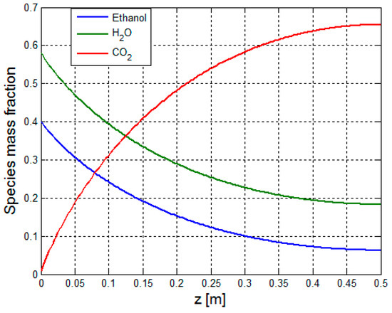
Figure 15.
Mass fractions of the species (ethanol, CO2 and H2O) along the reformer axis.
It can be seen from Figure 10 and Figure 15 that the mass fractions of ethanol and steam decay with increasing heat flux. The ethanol conversion is about 85.4%. Figure 16 shows the mass fractions of hydrogen along the reformer axis.
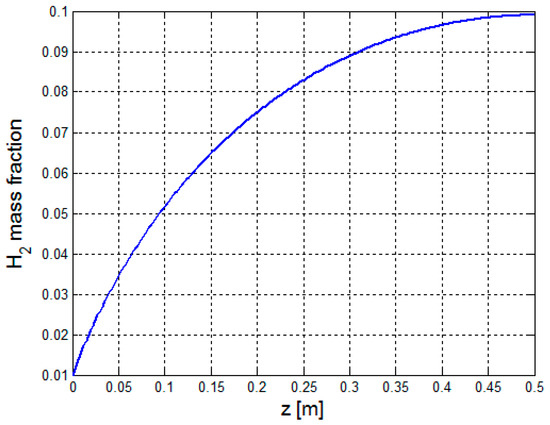
Figure 16.
Mass fractions of the H2 along the reformer axis.
Figure 16 indicates that the increase in hydrogen mass fraction is 89.9%. The hydrogen mass fraction is increased. Figure 17 shows the temperature distribution along the z axis of the reformer for the two cases.
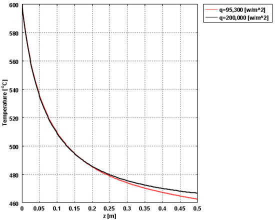
Figure 17.
Temperature distribution along the z axis of the reformer.
It can be seen from Figure 17 that the temperature increases with the increasing heat flux. As a result of that the hydrogen mass fraction increases (the reforming rate increases). The 3D Von-Mises stress distribution of reformer is shown in Figure 18.
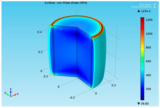
Figure 18.
3D plot of the reformer Von-Mises stress field.
Figure 19 shows the Von-Mises distribution along the z axis of the steel tube for the two cases.
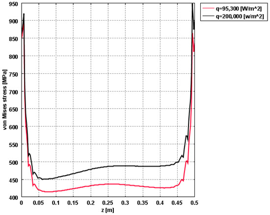
Figure 19.
Von-Mises distribution along the z axis of the steel tube.
Figure 19 indicates that Von-Mises stresses increases with the heat flux. The effect of increasing the heat fluxes increases the temperature inside the steel tube and enhances the thermal stresses. The thermal stresses which are developed inside the steel tube are much higher than those which were obtained in the previous section. The increase of the heat flux enhances a little the ethanol conversion, but also increases the thermal stresses developed inside the steel tube. This effect can cause to mechanical failure in the steel tube. In order to maintain the structural integrity of the tube, HK-40 alloy has been applied in this work. HK alloy, known as HK 40, is an austenitic Fe-Cr-Ni alloy that has been a standard heat resistant material with moderately high temperature strength, and oxidation resistance. Figure 20 shows the effect of temperature increasing on the tensile ultimate strength of HK 40 alloy and 310 stainless steels [30].
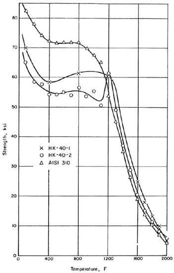
Figure 20.
The effects of the temperature on the ultimate tensile strength of HK 40 and 310 steels [28].
According to Figure 20, the maximal stress in the steel tube reached to maximal value of 482 MPa (70 ksi). From Figure 19 and Figure 20 it can be seen that the thermal stresses developed for low heat flux are much lower than the ultimate tensile strength of the HK-40 (According to Figure 20, the Von Mises stresses developed in the middle section of the tube are less than 450 MPa).
From Figure 20, it can be also seen that the decrease in the ultimate tensile strength is less than 10% (The temperature of the steel is about 600 °C or 1112 °F). Since ethanol steam reforming occurs at relatively lower temperatures compared with other hydrocarbon fuels, the decrease in the strength of the Steel tube is low. Therefore, the structural integrity of the HK-40 steel tube is kept. Figure 21 shows the effect of temperature stress rupture of HK 40-2 steel alloy [30].
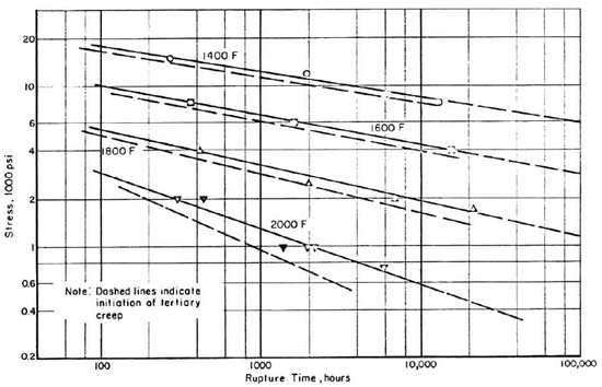
Figure 21.
The effects of the temperature on the rupture time of HK 40-2 alloy [30].
Figure 21 clearly indicates that under normal conditions of the ethanol reforming (the temperature of the steel tube is about 600 °C or 1112 °F), the rupture time increases considerably. For this case the rupture time is greater than 100,000 h (more than 11.4 years).
4. Discussion
Hydrogen could be a promising fuel, and if often considered as a clean energy carrier as it only emits water during combustion. It can be produced from different kinds of renewable feedstocks, such as ethanol. The use of ethanol as raw material presents several advantages because it is a renewable feedstock, easy to transport, biodegradable, has low toxicity, contains high hydrogen content, and easy to store and handle. Ethanol steam reformation occurs at relatively lower temperatures compared with other hydrocarbon fuels and has been widely studied due to the high yield provided for the formation of hydrogen. In this reformation reaction, water and ethanol react over a catalyst bed to produce a mixture of hydrogen rich gas. A new tool has been developed in this work in order to analyze the reformer operation. The proposed computational work is composed of two phases—simulation of ethanol burner by using FDS software and multiphysics simulation of steam reforming process occurring inside the reformer. This software calculates the temperature, density, pressure, velocity, and chemical composition within each numerical grid cell at each discrete time step. It computes the temperature, heat flux, and mass loss rate. There are three major components of the model: Hydrodynamic, combustion, and radiation models. FDS code is formulated based on CFD of fire-driven fluid flow. The FDS numerical solution can be carried out using either a DNS method LES. FDS uses a mixture fraction combustion model. The mixture fraction is a conserved scalar quantity that is defined as the fraction of gas at a given point in the flow field that originated as fuel. The model assumes that combustion is mixing controlled, and that the reaction of fuel and oxygen is infinitely fast. Radiative heat transfer is included in the model via the solution of the radiation transport equation for a non-scattering gray gas. The radiation equation is solved using a technique similar to a finite volume method for convective transport, thus the name given to it is the FVM. One advantage of FDS simulation is that it can provide much detailed information on the fire, including the local and transient gas velocity, gas temperature, species concentration, solid wall temperature, composite burning rate, radiation heat transfer, convection heat transfer and HRR. It has been found out that the maximal temperature at t = 77.5 s approaches to 815 °C. The magnitude of the radiation heat flux is 95,300 (w/m2).
The second part deals with numerical analysis of the reformer. The reformation chemical reactions occur in a porous catalytic bed where the heat is supplied through the Ethanol burner to drive the endothermal reaction system. The reactor is enclosed with a HK-40 alloy steel tube. Ethanol and steam are mixed in stoichiometric amounts and enter through the inlet of the catalytic reactor. The COMSOL multi-physics software has been applied in this work. It solved simultaneously the fluid flow, Heat transfer, diffusion with chemical reaction kinetics equations and structural mechanics. The diffusion equations values are obtained from the Chapman-Enskog theory. As far as I know, this work is the first CFD structural simulation study of ESR system. It is probably the first time that FDS software has been applied to simulate the ethanol burner.
A parametric study has been performed in order to analyze the influence of the heat flux on the reformer performance and its structural integrity. The numerical results were obtained for heat fluxes of 95,300 (W/m2) and 200,000 (W/m2). It is shown that the HRR produced by the ethanol burner, can provide the necessary heat flux required for maintaining the reforming process.
It has been found out that the mass fractions of the ethanol and steam decays along the reformer axis. The hydrogen and carbon dioxide mass fraction are increased along the reformer axis. The hydrogen mass fraction increases with enhancing the radiation heat flux. For the first case (heat flux magnitude of 95,300 (W/m2)) it was found out that the ethanol conversion is 80.3%. The ethanol and the steam are decaying at the same rate. Similar values have been reported in the literature. A sensitivity test has been carried out in order to analyze the influence of inlet temperature on ethanol conversion. The results show that for inlet temperature of 500 °C, the ethanol conversion is 70.0%. For inlet temperature of 400 °C, the ethanol conversion is 43.8%. Therefore, the ethanol conversion increases with the inlet temperature. There is a considerable increasing of Hydrogen mass fraction along the reformer axis. The increase in hydrogen mass fraction is 89.4%. The sum of hydrogen, ethanol, carbon dioxide and steam mass fraction at the reformer output is 1, as expected according the mass conservation law.
Similar physical behavior has been observed in the second case. The ethanol conversion is about 85.4%. The increase in hydrogen mass fraction along the reformer is 89.4%. The thermal stresses which are developed inside the steel tube are higher for the case of heat flux of 200,000 (W/m2). The increase of the heat flux enhances a little the ethanol conversion, but also increases the thermal stresses of the steel tube. This effect can cause to mechanical failure in the steel tube. In order to maintain the structural integrity of the tube, HK-40 alloy has been applied in this work. HK alloy, known as HK 40, is an austenitic Fe-Cr-Ni alloy that has been a standard heat resistant material with moderately high temperature strength, and oxidation resistance. This alloy is used in a wide variety of industrial applications such as: Ammonia, methanol, and hydrogen reformers; ethylene pyrolysis coils and fittings; and steam super heater tubes and fittings.
It has been found out that by increasing the heat flux of the reformer, the decrease in the tensile yield strength of HK-40 alloy is less than 10% (the temperature of the steel is about 600 °C or 1112 °F). The effect of increasing the heat fluxes increases the temperature inside the steel tube and enhances the thermal stresses (produced by the thermal expansion). Since ethanol steam reforming occurs at relatively lower temperatures compared with other hydrocarbon fuels, the decrease in the strength of the steel tube is low. Thus, the structural integrity of the HK-40 steel tube is kept.
The numerical results for clearly indicates that under normal conditions of the ethanol reforming (the temperature of the steel tube is about 600 °C or 1112 °F), the rupture time increases considerably. For this case the rupture time is greater than 100,000 h (more than 11.4 years). The described algorithm described in this work may be applied other reformer system (diesel, methanol, or methane).
5. Conclusions
A new tool has been developed in this work in order to analyze the burner and steam reformer operation. This model may be implemented for simulating other reforming systems (such as methanol, and diesel). Future work will focus on performing coupled heat transfer, chemical reactions, and creep analyses on the reformer.
Funding
This research received no external funding.
Conflicts of Interest
The author declares no conflict of interest. No funding sponsors had any role in the numerical analyses, or interpretation of data; in the writing of the manuscript, and in the decision to publish the results.
References
- Poran, A.; Tartakovsky, L. Performance and emissions of a direct injection internal combustion engine devised for joint operation with a high-pressure thermochemical recuperation system. Energy 2017, 124, 214–226. [Google Scholar] [CrossRef]
- Akande, A.; Aboudheir, A.; Idem, R.; Dalai, A. Kinetic modeling of hydrogen production by the catalytic reforming of crude ethanol over a co-precipitated Ni-Al2O3 catalyst in a packed bed tubular reactor. Int. J. Hydrogen Energy 2006, 31, 1707–1715. [Google Scholar] [CrossRef]
- Marino, F.; Boveri, M.; Baronetti, G.; Laborde, M. Hydrogen production from steam reforming of bioethanol using Cu/Ni/K/γ-Al2O3 catalysts. Effect of Ni. Int. J. Hydrogen Energy 2001, 26, 665–668. [Google Scholar] [CrossRef]
- Bineli, A.R.; Tasić, M.B. Catalytic Steam Reforming of Ethanol for Hydrogen Production: Brief Status. Chem. Ind. Chem. Eng. Q. 2016, 22, 327–332. [Google Scholar] [CrossRef]
- Akande, A.J. Production of Hydrogen by Reforming of Crude Ethanol. Master’s Thesis, University of Saskatchewan, Saskatoon, SK, Canada, 2005. [Google Scholar]
- Athanasios, N.F.; Kondaridesm, D.I. Production of hydrogen for fuel cells by reformation of biomass-derived ethanol. Catal. Today 2002, 75, 145–155. [Google Scholar]
- Klouz, V.; Fierro, V.; Denton, P.; Katz, H.; Lisse, J.P.; Bouvot-mauduit, S.; Mirodatos, C. Ethanol reforming for hydrogen production in a hybrid electric vehicle: Process optimization. J. Power Sources 2002, 105, 26–34. [Google Scholar] [CrossRef]
- Uriz, I.; Arzamendi, G.; López, E.; Llorca, J.; Gandía, L.M. Computational fluid dynamics simulation of ethanol steam reforming in catalytic wall micro channels. Chem. Eng. J. 2011, 167, 603–609. [Google Scholar] [CrossRef]
- Uriz, I.; Arzamendi, G.; Diéguez, P.M.; Gandía, L.M. Computational fluid dynamics as a tool for designing hydrogen energy technologies. In Renewable Hydrogen Technologies: Production, Purification, Storage, Applications and Safety; Elsevier: Oxford, UK, 2013; Chapter 17; pp. 401–435. [Google Scholar]
- Lao, L.; Aguirre, A.; Tran, A.; Wu, Z.; Durand, H.; Christofides, P.D. CFD modeling and control of a steam methane reforming reactor. Chem. Eng. Sci. 2016, 148, 78–92. [Google Scholar] [CrossRef]
- Lewis, B.; Von Elbe, G. Combustion Flames and Explosion of Gases, 2nd ed.; Academic Press Inc.: New York, NY, USA; London, UK, 1961. [Google Scholar]
- Diéguez, P.M.; López-San, M.J.; Idareta, I.; Uriz, I.; Arzamendi, G.G.; Luis, M. Hydrogen Hazards and Risks Analysis through CFD Simulations. In Renewable Hydrogen Technologies: Production, Purification, Storage, Applications and Safety; Elsevier: Oxford, UK, 2013; Chapter 18; pp. 437–452. [Google Scholar]
- Tartakosky, L.; Sheintoch, M. Fuel Reforming in Internal Combustion Engines. Prog. Energy Combust. Sci. 2018, 67, 88–114. [Google Scholar] [CrossRef]
- European Industrial Gases Association AISBL. Combustion Safety for Steam Reformer Operation; IGC Doc 172/12/E; European Industrial Gases Association AISBL: Brussels, Belgium, 2012. [Google Scholar]
- Olafadehan, O.A.; Ayoola, A.A.; Akintunde, O.O.; Adeniyi, V.O. Mechanistic Kinetic Models for Steam Reforming of Concentrated Crude Ethanol on Ni/Al2O3 Catalyst. J. Eng. Sci. Technol. 2015, 10, 633–653. [Google Scholar] [CrossRef]
- Loock, S.; Ernst, W.S.; Thomsen, S.G.; Jensen, M.F. Improving Carbon Efficiency in an Auto-Thermal Methane Reforming Plant with Gas Heated Heat Exchange Reforming technology. In Proceedings of the 7th World Congress of Chemical Engineering, Glasgow, UK, 10–14 July 2005. [Google Scholar]
- Carlsson, M. Carbon Formation in Steam Reforming and Effect of Potassium Promotion. Johnson Matthey Technol. Rev. 2015, 59, 313–318. [Google Scholar] [CrossRef]
- Heywood, J.B. Internal Combustion Engine Fundamentals; McGraw-Hill Book Company: New York, NY, USA, 1988. [Google Scholar]
- McGrattan, K. Fire Dynamics Simulator (Version 5)—Technical Reference Guide Volume 1: Mathematical Model; NIST Special Publication 1018; National Institute of Standards and Technology U.S. Department of Commerce: Gaithersburg, MD, USA, 2010.
- McGrattan, K.; Forney, G.P. Fire Dynamics Simulator (Version 5)—User’s Guide; NIST Special Publication 1019; National Institute of Standards and Technology U.S. Department of Commerce: Gaithersburg, MD, USA, 2010.
- McGrattan, K. Numerical Simulation of the Caldecott Tunnel Fire, April 1982; NISTIR 7231; National Institute of Standards and Technology U.S. Department of Commerce: Gaithersburg, MD, USA, 2005.
- Hu, L. A review of physics and correlations of pool fire behavior in wind and future challenges. Fire Saf. J. 2017, 91, 41–55. [Google Scholar] [CrossRef]
- Hamins, A.; Kashiwagi, T.; Bruch, R.R.; Toten, G.E. Fire Resistance of Industrial Fluids, ASTM STP 1284; Toten, G.E., Reichel, J.E., Eds.; American Society for Testing and Materials: Philadelphia, PA, USA, 1995. [Google Scholar]
- Thermo-Physical Properties of Ethanol. Available online: https://www.thermalfluidscentral.org/encyclopedia/index.php/Thermophysical_Properties:_Ethanol (accessed on 8 June 2018).
- De-Souza, Z.G.M.; Moraes, F.F. Parametric Study of Hydrogen Production from Ethanol Steam Reforming in Membrane Micro-reactor. Braz. J. Chem. Eng. 2013, 30, 355–367. [Google Scholar] [CrossRef]
- Neufeld, P.D.; Jansen, A.R.; Aziz, R.A. Empirical equations to calculate 16 of the transport collision integrals Ω(l,s)* for the Lennard-Jones (1216–) potential. J. Chem. Phys. 1972, 57, 1100–1102. [Google Scholar] [CrossRef]
- Perry, R.H.; Green, D.W.; Maloney, J.O. Perry’s Chemical Engineers’ Handbook, 7th ed.; McGraw Hill: New York, NY, USA, 1997. [Google Scholar]
- Kubota Metal Corporation. Fahramet Division, Alloy Data Sheet, Heat Resistant Alloy HK40; Kubota Metal Corporation: Orillia, ON, Canada, April 1991. [Google Scholar]
- Steel Founders’ Society of America. Steel Casting Handbook; Supplement 9, High Alloy Data Sheets Heat Series; Steel Founders’ Society of America: Crystal Lake, IL, USA, 2004. [Google Scholar]
- Van Echo, J.A.; Roach, D.B.; Hall, A.M. Short Time Tensile and Long-Time Creep Rupture Properties of the HK-40 Alloy and Type 310 Stainless Steel at Temperature to 2000 °C. ASME J. Basic Eng. Trans. 1967, 89, 465–478. [Google Scholar] [CrossRef]


© 2018 by the author. Licensee MDPI, Basel, Switzerland. This article is an open access article distributed under the terms and conditions of the Creative Commons Attribution (CC BY) license (http://creativecommons.org/licenses/by/4.0/).