Article

Predicting of Daily PM2.5 Concentration Employing Wavelet Artificial Neural Networks Based on Meteorological Elements in Shanghai, China

1
School of Geography and Environment, Liaocheng University, Liaocheng 252000, China
2
Institute of Huanghe Studies, Liaocheng University, Liaocheng 252000, China
3
State Key Laboratory of Loess and Quaternary Geology, Institute of Earth Environment, Chinese Academy of Sciences, Xi’an 710061, China
4
State Key Laboratory of Urban and Regional Ecology, Research Center for Eco-Environmental Sciences, Chinese Academy of Sciences, Beijing 100085, China
5
Ecosystem Science Data Center, Key Laboratory of Ecosystem Network Observation and Modeling, Institute of Geographic Sciences and Natural Resources Research, Chinese Academy of Sciences, Beijing 100101, China
*
Authors to whom correspondence should be addressed.
Toxics 2023, 11(1), 51; https://doi.org/10.3390/toxics11010051
Submission received: 24 November 2022 / Revised: 30 December 2022 / Accepted: 2 January 2023 / Published: 3 January 2023
(This article belongs to the Special Issue Air Pollution and COVID-19)

Abstract

:
Anthropogenic sources of fine particulate matter (PM2.5) threaten ecosystem security, human health and sustainable development. The accuracy prediction of daily PM2.5 concentration can give important information for people to reduce their exposure. Artificial neural networks (ANNs) and wavelet-ANNs (WANNs) are used to predict daily PM2.5 concentration in Shanghai. The PM2.5 concentration in Shanghai from 2014 to 2020 decreased by 39.3%. The serious COVID-19 epidemic had an unprecedented effect on PM2.5 concentration in Shanghai. The PM2.5 concentration during the lockdown in 2020 of Shanghai is significantly reduced compared to the period before the lockdown. First, the correlation analysis is utilized to identify the associations between PM2.5 and meteorological elements in Shanghai. Second, by estimating twelve training algorithms and twenty-one network structures for these models, the results show that the optimal input elements for daily PM2.5 concentration predicting models were the PM2.5 from the 3 previous days and fourteen meteorological elements. Finally, the activation function (tansig-purelin) for ANNs and WANNs in Shanghai is better than others in the training, validation and forecasting stages. Considering the correlation coefficients (R) between the PM2.5 in the next day and the input influence factors, the PM2.5 showed the closest relation with the PM2.5 1 day lag and closer relationships with minimum atmospheric temperature, maximum atmospheric pressure, maximum atmospheric temperature, and PM2.5 2 days lag. When Bayesian regularization (trainbr) was used to train, the ANN and WANN models precisely simulated the daily PM2.5 concentration in Shanghai during the training, calibration and predicting stages. It is emphasized that the WANN1 model obtained optimal predicting results in terms of R (0.9316). These results prove that WANNs are adept in daily PM2.5 concentration prediction because they can identify relationships between the input and output factors. Therefore, our research can offer a theoretical basis for air pollution control.

1. Introduction

Air pollution affects global climate change, ecosystem and human health [1,2,3,4,5]. Additionally, air pollution also leads to huge losses in human capital, productive forces and social welfare [6]. Air pollution is responsible for millions of deaths all over the world [7]. Exposure to air pollution resulted in 7 million premature deaths all over the whole world in 2019 [8]. In total, 1.42 million deaths in China were ascribed to outdoor air pollution in 2019 [9]. High concentration of PM2.5 are associated with reduced visibility, economic loss and passive impact on public health because it adds to the incidence rate and mortality of some diseases [10]. Global exposure to environmental PM2.5 causes about ~6 to ~10 million deaths every year [6]. In total, 2.12 million deaths in China in 2017 were attributed to PM2.5 [11]. Therefore, the accurate prediction of future air pollution can offer reference for travel mode.
With the rapid development of China’s economy, a lot of fossil energy is consumed. Meanwhile, a large number of polluting gases and particulate matter are emitted into the air, seriously influencing the air on which human beings depend. Air pollution is mainly caused by abundant pollutant emissions [12]. It is also strongly related to meteorological conditions [13,14]. The removal and dissipation of air pollutants is determined by the atmospheric diffusion conditions and the precipitation [15].
The outbreak of the COVID-19 pandemic has had a negative impact on social and economic development and human health [16,17]. On 30 January 2020, the WHO Emergency Committee designated COVID-19 as a global health emergency; as of 12 August 2022, COVID-19 had caused at least 585,950,085 confirmed cases and 6,425,422 deaths globally (WHO). The COVID-19 epidemic has had an unprecedented influence on global air pollution [18,19,20,21,22,23]. The abrupt COVID-19 pandemic offers a chance to research the impact of urban blockade policies on the change of air pollutants, and to describe the normal modes of air pollution under the disappearance of the epidemic [24]. The COVID-19 epidemic has had an unprecedented influence on the air pollution in the Beijing and Tianjin districts [25]. During the period of the COVID-19, different urban blockade policies significantly improved the air quality of all four mega cities in China [26]. The reduction of social and productive activities during the lockdown plays an extraordinarily significant role in improving air quality [27]. The implementation of travel restrictions greatly reduced air pollution in 44 cities in China. In addition, the concentration of PM2.5 decreased by 5.93% [28]. Air quality can be improved by emphasizing the importance of green commuting, green production and consumption and reducing unnecessary personal trips.
Air pollution forecasting techniques include numerical models and statistical models [29]. The numerical models achieve the simulation of the transformation and diffusion of air pollutants and reflect the change law of air pollutants. However, they are based on a large amount of meteorological information, air pollutant discharge source data and atmospheric monitoring data, they need to master the mechanism of pollution change, and the calculation time is long [30]. Daily PM2.5 concentration prediction is a nonlinear, multivariable problem with strong coupling between predictors, so PM2.5 numerical forecasting will be an extraordinarily complex system engineering problem. Statistical models are widely used in operational prediction, with the strong points of easy calculation, low data requirements and high precision. Nevertheless, most statistical models align with linear regression theory; assuming that there is nonlinear relationship between pollutant concentration and weather conditions, linear regression is difficult to be applied to nonlinear strongly coupled systems [31]. So far, the artificial intelligence (AI) technique has been extensively applied in a variety of research areas [32,33,34,35].
Machine learning (ML) is an important branch discipline of AI which has been extensively utilized in many research areas [36]. The chief aim of ML is to automatically optimize the nature of algorithms through emulating historical data. ML is able to build steady models, learning from historical data, and utilize these models to forecast future data. Machine learning methods, such as artificial neural networks (ANNs) [37], support vector machines (SVMs), and extreme gradient boosting (XGBoost), have shown fine performance in dealing with nonlinear problems. Deep learning (DL) has also been extensively applied in various fields [38,39]. For example, ordinary recurrent neural networks (RNNs) and convolutional neural networks (CNNs) are usually employed to predict air pollution [40].
Previous researchers have put forward different ML algorithms used for data modeling. Some researchers have proved that ANN has good learning efficiency and is extensively utilized in forecasting groundwater level [41], the COVID-19 epidemic [42], air pollution [43,44], and so on. There is good similarity in the predictive and metrical PM2.5 for training in the ANN [45].
Although the deep neural network is powerful, it still has many shortcomings. First, there are too many parameters in DNN, and the learning performance depends heavily on careful parameter adjustment. Secondly, the training of DNN requires a large amount of training data, so it is laborious to apply DNN to tasks with only small-scale training data [46]. In addition, the challenges faced by DL are more common, such as the deficiency of theoretical basis, the insufficiency of interpretability of models, and the need for big amounts of computing resources [47].
There are various types of mother wavelet functions. According to the diurnal variation of air pollutant concentration, each wavelet has its pros and cons in the air pollutant concentration decomposition properties [48]. Using wavelet transform to transform highly variable air pollutant concentrations into several low variability subsequences has distinct merits. For most models, wavelet transform is an effective technique to increase the forecasting accuracy [49]. The basic prediction model uses wavelet transform to decompose the air pollutant concentrations, and then uses artificial neural networks to predict it.
This paper proposes a hybrid model of wavelet transform and ANN (WANN) solution to the problem of predicting the daily PM2.5 concentration. To avoid overfitting, the improved algorithms are utilized for modeling, such as trainbr and trainlm. The hybrid model provides a novel alternative for forecasting daily PM2.5 concentration.

2. Materials and Methods

2.1. Study Location and Data Sources

Shanghai is the largest city in China (Figure 1a). Shanghai is located in East China with the area of 6340 km2, and it is at the estuary of the Yangtze River. The average altitude of Shanghai is 2.19 m, and the permanent resident population and the GDP in 2021 were about 24.8943 million and CNY 4321.485 billion.
In this paper, the air pollution data sets and meteorological data sets of Shanghai from 1 January 2014 to 31 December 2020 are utilized. The daily PM2.5 concentration data are from the mean values of twenty monitoring sites (stations) in Shanghai and can be obtained on the website of China Environmental Monitoring Station (http://www.cnemc.cn/) (accessed on 21 January 2022) and platform (http://www.aqistudy.cn/) (accessed on 22 January 2022) (Figure 1b). Table 1 displays the list of the monitoring stations used in this study. The data of meteorological elements (including temperature, precipitation, humidity, wind, atmospheric pressure, etc.) are from the average value of the observation station of the China Meteorological Administration. These data are divided into three stages, namely, the training stage (80%), the verification stage (10%) and the prediction stage (10%). The training stage is from 1 January 2014 to 30 June 2019, the verification stage is from 1 July 2019 to 31 March 2020, and the prediction stage is from 1 April 2020 to 31 December 2020.

2.2. Wavelet Transformation (WT)

Wavelet transformation (WT) is one of the waveform analytical methods for time-varying signals. In wavelet transform, the wavelet coefficients can be obtained by convolution integration of the mother wavelet function and the original time domain signal. Discrete wavelet transform (DWT) has the advantage of less computational expense than continuous wavelet transform (CWT). The Daubechies (db) wavelet is the most commonly utilized mother wavelet function. The Mallat pyramidal algorithm is used to compute DWT. Therefore, the DWT is used to decompose the daily PM2.5 concentration data and meteorological elements data [50]. The DWT of a time series f(q) is defined as Equation (1):
f ( c , d ) = 1 c f ( h ) ψ ( h d c ) d h
where ψ(h) expresses the fundamental wavelet of effective length h; c expresses the scale or dilation factor; and d expresses the translation time. For a discrete signal y, the DWT is defined by multi-resolution decomposition, which can be computed by the Mallat decomposition algorithm and Mallat pyramidal reconstruction algorithm [41]. For m-level decomposition and reconstruction, the original signal y can be expressed as
y = CA m + i = 1 m C D i
where CAm is the approximation series representing the low-frequency component, which contains trend information, and CDi is the detail series on the i level representing the high-frequency component, which contains periodic information. Basically, this is a process in which the low-frequency sequence is decomposed into low-frequency subsequences and relatively high-frequency subsequences with the increase in m (Figure 2). The results of the 2-level wavelet decomposition of the original time series of PM2.5 concentration by applying bior1.1 wavelets was implemented in the wavelet toolbox of MATLAB.
The main purpose of utilizing the discrete wavelet transform is to reduce the complexity of the input signal and the amount of relevant information between the decomposition combinations (detailed CD2, CD1 and approximate CA2). Discrete wavelet transform could be used to approximate components to obtain low dimensional components and gain components for multidimensional analysis.

2.3. Artificial Neural Network (ANN)

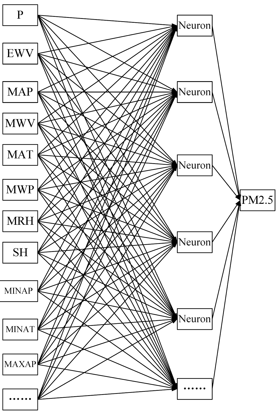
An artificial neural network (ANN) is a part of AI. It simulates the prediction and recognition functions of the biological brain and is used to solve complex problems in various application fields. The typical network architecture of an ANN consists of three layers (i.e., input layer, hidden (implication) layer and output layer), each one composed of several artificial neurons and an activation function. Each artificial neuron is contacted via weights and gains information from the correlative neurons for processing. Owing to its strong nonlinear processing features, ANN could output nonlinear relationships of many complicated scientific problems. The proposed ANN model for predicting the daily PM2.5 concentration is displayed in Figure 3. The seventeen input neurons of the input layer are designed as the key operating parameters, which include precipitation (P), extreme wind velocity (EWV), mean atmospheric pressure (MAP), mean wind velocity (MWV), mean atmospheric temperature (MAT), mean water vapor pressure (MWP), mean relative humidity (MRH), sunshine hours (SH), minimum atmospheric pressure (MINAP), minimum atmospheric temperature (MINAT), maximum atmospheric pressure (MAXAP), maximum atmospheric temperature (MAXAT), maximum wind velocity (MAXWV), minimum relative humidity (MINRH), PM2.5 (t), PM2.5 (t − 1), and PM2.5 (t − 2).
Back propagation (BP) is the most commonly used and effective method to train the artificial neural network (ANN) algorithm. In the process of model development, there are two phases of forward propagation and error back propagation. The hidden (implication, middle) layer neurons calculate the weighted summation of the acquired input layer information s using Equations (3) and (4), and transmit these to the coming layer through the activation function (transfer function), then contrast the error criterions between the input value and the metrical value, then transfer the error back to the input layer, and decrease the error to the goal standard by altering the relation weight and thresholds (deviations or biases) [51].
k = i = 1 m w i j O i + p
Q = f ( k )
where k is the weighted total, wij is the relation weight, j is the number of neurons in the output layer, Oi is the input data, and p is the biases (deviation or thresholds) value, utilized to balance the effect of the activation function. Q is the output data, and f is the activation function. After the forward propagation transversion of the signals, the global error is counted. If the global error is lower than the setting error (10−5), the backward propagation of the global error is completed to change the weights and thresholds. The back propagation of the global error function is counted as in Equation (5):
E = 1 l j = 1 l ( T j Q j ) 2
where E is the error of the current output, Tj is the target output, Qj is the predicted output, and l is the total output number (2004). After adjusting and training the network model, the messages of the input parameters could be stored for modelling, such as weights and thresholds (biases).
Four kinds of activation functions are usually utilized in BPANN are sigmoid (logsig), tanh (tansig), purelin and ReLU (poslin) functions, which are logarithmic sigmoid, hyperbolic tangent sigmoid, linear, and positive linear transfer functions, respectively. The four functions of the network are defined as follows:
s i g m o i d ( r ) = 1 1 + e r
t a n s i g ( r ) = e r e r e r + e r
p u r e l i n ( r ) = r
R e L U ( r ) = 0 , i f ( r 0 ) r , i f ( r 0 )
where r is the corresponding input.
Artificial neural networks could fulfil well in the training information, but not well in the forecasting information, which explains that they perform poorly as different information or error increases. When the artificial neural network (ANN) cannot generalize this problem, it is called “overfitting”. This problem could be solved utilizing the Bayesian regularization algorithm (BR, or trainbr), Levenberg–Marquardt algorithm (LM, or trainlm) or other training algorithms [52]. Trainbr is a function which updates weights and threshold (bias or deviation) values on the basis of LM optimization. It minimizes the union of square error and weight, and then ascertains the correct union to generate a network with good generalization. In addition, the LM algorithm (trainlm) is a variant of Newton’s way, which is devised to minimize the sum of squares of other nonlinear functions. While the property function has the modality of the summation of squares, the Hessian matrix could be calculated approximately as the outcome of the Jacobian matrix, which is much less complicated than calculating the Hessian matrix.
The raw data were normalized, for quick convergence, and rendered dimensionless. The results after treatment are as follows:
S = s s min s max s min
where S is the normalized data for the original variable, smin is the minimum of the raw data, smax is the maximum of the raw data, and s denotes the original data.

2.4. Wavelet Artificial Neural Network

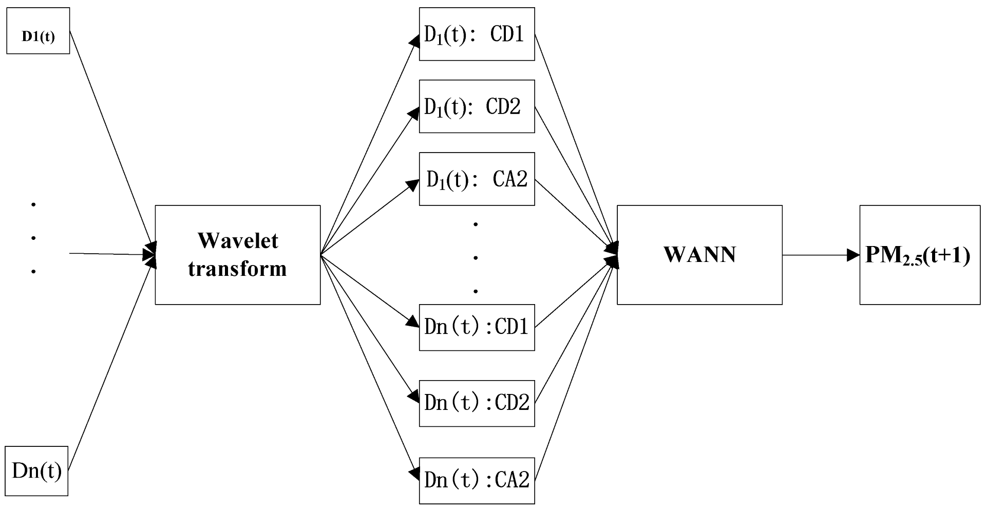
The WANN model is utilized to decompose the raw data Dn (t) into three suites: CD2, CD1 and CA2. After that, these data are employed by the ANN as the input factors. In Figure 4, Dn (t) is the input factors of day t, PM2.5 (t + 1) is the PM2.5 predicted t + 1 day in the future.

2.5. Performance Criteria

Three kinds of statistical indicators were adopted to appraise the nature of ANN and WANN models. These are mean absolute error (MAE), root mean square error (RMSE), and correlation coefficient (R), which are as follows:
M A E = 1 U A k C k
R M S E = ( A k C k ) 2 U
R = ( A k A ) ( C k C ) ( A k A ) 2 ( C k C ) 2
Ak expresses the kth observed PM2.5 concentration, Ck expresses the kth predicted PM2.5 concentration, A is the mean of the observed PM2.5 concentration, C is the mean of the predicted PM2.5 concentration, and U is the number of observed PM2.5 concentration.

3. Result and discussion

3.1. Long Term Change of PM2.5 Concentration in Shanghai

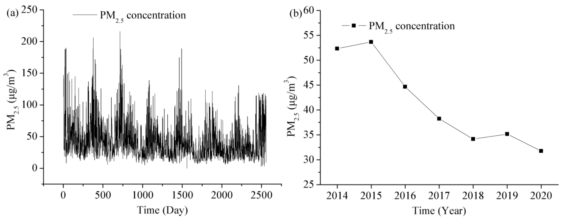
As shown in Figure 5, the PM2.5 concentration in Shanghai shows a tendency of descending year after year. The annual mean PM2.5 concentrations from 2014 to 2020 are 52.33 μg/m3, 53.67 μg/m3, 44.67 μg/m3, 38.25 μg/m3, 34.17 μg/m3, 35.17 μg/m3, and 31.75 μg/m3, in the range of 8–190 μg/m3, 6–216 μg/m3, 5–163 μg/m3, 7–175 μg/m3, 6–189 μg/m3, 6–122 μg/m3, and 3–131 μg/m3, respectively. The PM2.5 concentration in Shanghai decreased by 39.3% from 2014 to 2020. This change improved the PM2.5 level from about 10 times the World Health Organization (WHO) guidelines to about 6 times. The average value of PM2.5 concentration in Shanghai for the 7 years is 41.43 μg/m3. Although the air quality in Shanghai has improved a lot, it exceeded the new Global Air Quality Guidelines (AQGs) of the WHO standard (5 μg/m3 above the annual PM2.5 limit). The average value change of PM2.5 in 7 years has a U-shaped characteristic, with the maximum in January and the minimum in August. The seasonal average value of PM2.5 in 7 years has obvious change characteristics, with the maximum in winter, followed by spring, autumn and the minimum in summer.
The COVID-19 epidemic has had a significant impact on the PM2.5 concentration in Shanghai. These data in 2019–2020 are divided into three parts: period I (1 January to 26 January, 2019–2020); period II (27 January to 30 April, 2019–2020); and period III (1 May to 31 July, 2019–2020). Period II is the lockdown period. The values of PM2.5 during period I, period II, and period III in 2020 are, respectively, 52.62, 32.41, and 31.99 (μg/m3). However, those are, respectively, 53.12, 43.11, and 29.58 (μg/m3) in the same period of 2019. Compared with those values in 2019, these values of PM2.5 in 2020 decreased by 0.5, 10.7, and −2.41 (μg/m3), which are respectively 0.9, 24.8, and −8.2% lower in 2020 than those in 2019. The air quality during lockdown in 2020 is apparently improved compared with that in the same period of 2019.

3.2. Relevance between Daily PM2.5 Concentration and Meteorological Factors in Shanghai

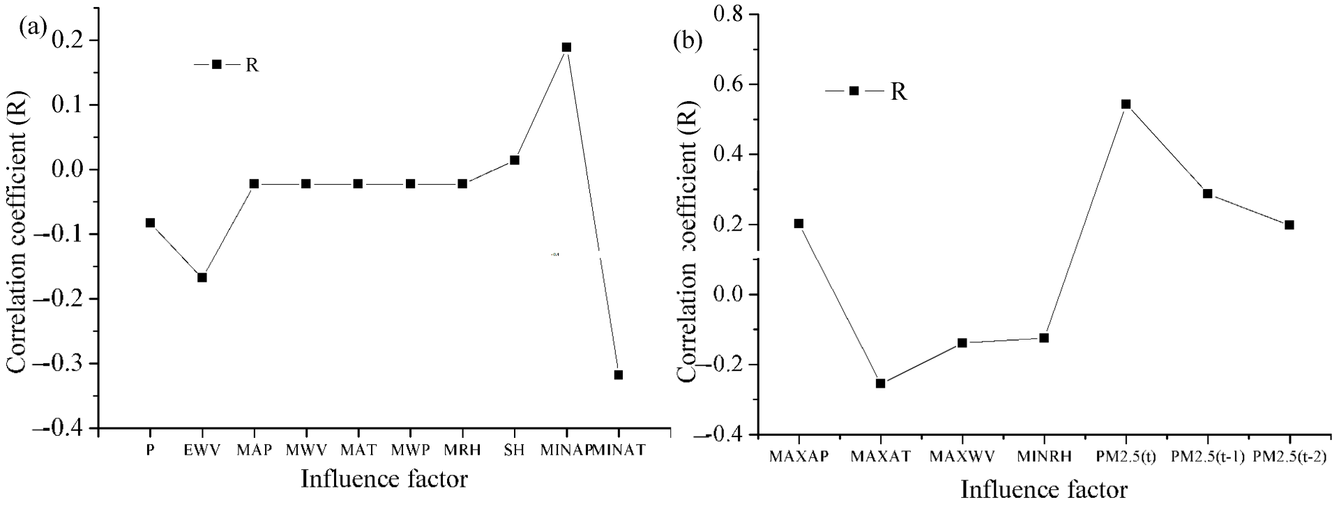
Correlation analysis could ascertain the linear relationships between PM2.5 concentration and meteorological elements. The determination of input variables is one of the most significant parts in the projection of ANN and WANN models. The results of the relationships counted for the input factors are shown in Figure 6, which is significant at the 0.01 level (2-tailed).
The correlation between each factor and PM2.5 (t + 1) was appraised by determining its R. The analysis results exhibited that PM2.5 (t) was strongly related to PM2.5 (t + 1) in Shanghai. In addition, the performance results of MINAT, MAXAP, MAXAT, PM2.5 (t), PM2.5 (t − 1) were better than other factors in Shanghai. That is, these meteorological factors have the highest correlation to PM2.5 (t + 1). We ascertained five important factors. Therefore, various combinations of factors were used as inputs for simulating daily PM2.5 (t + 1) in Table 2. For example, the network structure 17:5:1 in Table 1 indicates that there are 17 neurons in the input layer, 5 neurons in the hidden layer, and 1 neuron in the output layer. Other network structures are similar. The ascertaining factors were chosen based on relationship with PM2.5.

3.3. Determination of Model Structure and Parameters

It should be stressed that selecting the most compatible network structure is one of the important assignments of the model designer. The important information obtained from meteorological elements is extracted by discrete wavelet transform (DWT). The various details and dimensions of input factors are gained by two-period decomposition of WT. After two-period decomposition and reconstruction, the input factors are changed into three parts. The approximate component CA2 represents the low frequency information of the raw factor, while the detailed CD2 and CD1 represent the high-frequency information of the raw factor. The change characteristics of time series are the key factors affecting wavelet selection [53]. In order to optimize the decomposition of input factors, the mother wavelet is chosen, and the correlation between CD1, CD2 and CA2 is considered. The minimum R could primely meet the objective of analyzing the change characteristics of various components of input factors. The quantitative estimation showed that the components were independent of one another. In total, 21 types of wavelet functions are ascertained for wavelet transform. The mother wavelets (wavelet functions) evaluated are Daubechies (db), symlets (sym), coiflets (coif), and biorthogonal wavelets (bior) [54]. Coiflets are a family of compactly supported orthogonal wavelets. Figure 7 shows that bior1.1 is the best wavelet function in the current research on account of the smallest R. bior1.1 is a biorthogonal wavelet [54]. The correlation coefficients between CD1, CD2 and CA2 after the input factors are decomposed by bior1.1 are all 0.
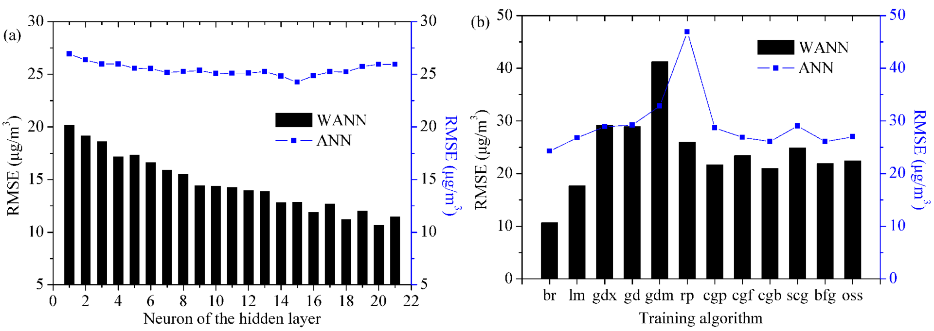
The optimal model parameters are obtained by the trial-and-error method. Figure 8 demonstrates that the network structures (17-15-1 for ANN and 51-20-1 for WANN) are superior to other network topologies through repeated tests. In the models, the number of neurons of the hidden (implication, middle) layer increases from 1 to 21. It can be seen from Figure 6 that the RMSE value decreases slightly with the increase in the number of hidden (implication, middle) layer neurons. Consequently, the optimal structures of the mode for Shanghai are 17-15-1 (ANN) and 51-20-1 (WANN), respectively.
Figure 8 expresses the properties of the training algorithms, indicating that the trainbr algorithm has the best property in forecasting PM2.5 (t + 1) in Shanghai. Trainbr automatically fits the optimal values of the objective function parameters.
Figure 9 shows that the activation function (tansig-purelin) for ANN in Shanghai is better than others during training, calibration and predicting stages. In the same way, the transfer function (tansig-purelin) for WANN in Shanghai is also better than others in Figure 9.

3.4. Comparative Analysis of the Different PM2.5 Predicting Models

All results of the ANNs and WANNs during the training, validation and predicting stage are shown in Table 3. We used the ten-fold cross-validation method to verify the models. During the training stage, the root mean square errors (RMSEs) of ANN1 and WANN1 in Shanghai were 20.7841 and 9.8824, respectively; mean absolute errors (MAEs) were 15.0825 and 7.1153, respectively; and correlation coefficients (Rs) were 0.7061 and 0.9416, respectively. In the meantime, RMSE, MAE, and R for ANN2, ANN3, ANN4, WANN2, WANN3, and WANN4 have similar results. During the training stage, the WANNs were superior to the ANNs. During the verification stage, the RMSEs of ANN1 and WANN1 in Shanghai were 17.0006 and 9.7850, respectively; MAEs were 13.1262 and 6.8827, respectively; and Rs were 0.6830 and 0.8969, respectively. During the predicting stage, the RMSEs of ANN1 and WANN1 in Shanghai were 24.2407 and 10.6580, respectively; MAEs were 17.7867 and 7.6918, respectively; and Rs were 0.5618 and 0.9316, respectively. In the above three stages, the WANNs were also superior to the ANNs. The WANN1 model based on all 17 input variables is the best model in predicting PM2.5 concentration. The WANN2 model based on five input variables is the second-best model for predicting PM2.5 concentration. It is interesting that the performance of WANN2 is similar to WANN1. These two models can meet the PM2.5 concentration prediction requirements.
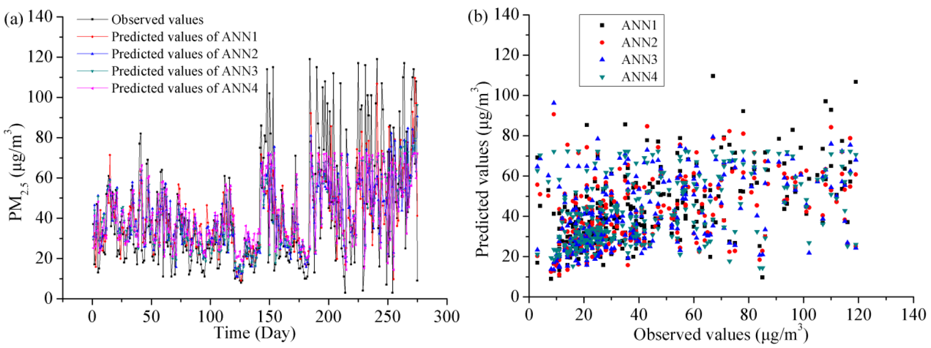
Figure 10 displays the forecasting PM2.5 outcomes and scatter plots with the ANN models in the testing stage in Shanghai. ANNs were able to replicate the average of the daily PM2.5 concentration but were limited in capturing minimal or maximal peaks. However, the predicted and observed values are relatively scattered.
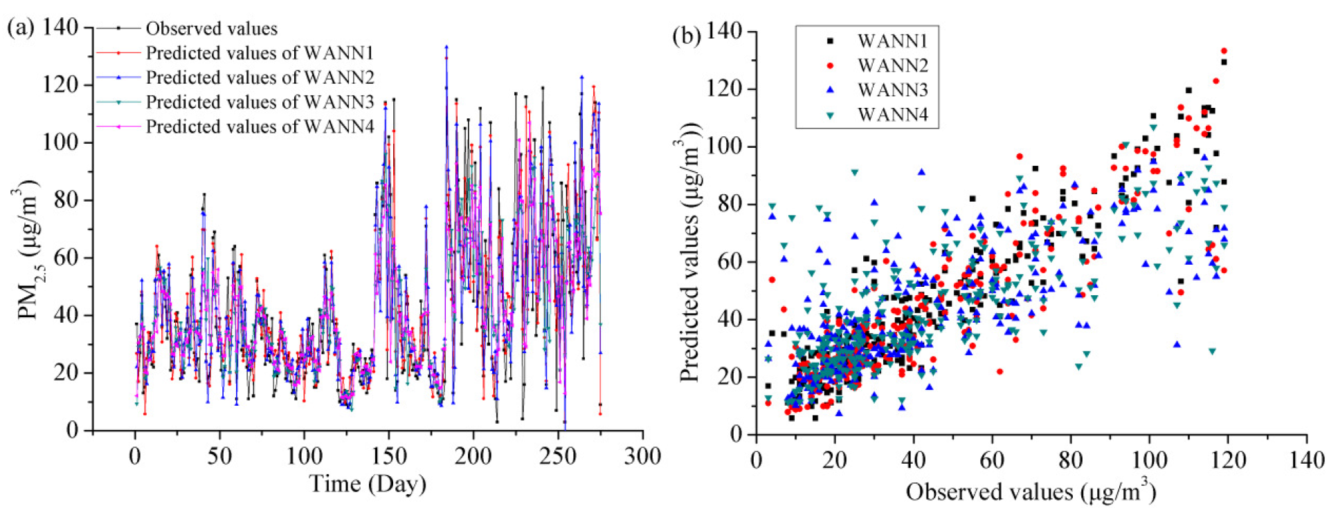
Figure 11 indicates the forecasting line and scatter plots with the WANNs in the testing stage. The WANNs predicted daily PM2.5 concentration at an acceptable precision level in Shanghai. Additionally, WANNs were apparently superior to ANNs. The WANNs reproduced a good consistency between the observed PM2.5 (t + 1) concentration and predicted PM2.5 (t + 1) concentration. It is also apparent that the WANN1 model with 14 meteorological elements was better than the WANN4 with 1-day lag PM2.5 concentration; in other words, including 14 meteorological elements and the 3 former days’ PM2.5 as parameters in the input factors supplies more precise results. The agreement between the observed PM2.5 (t + 1) concentration and the predicted PM2.5 (t + 1) concentration is also very good in Shanghai using the WANN2 model. The main meteorological elements of the WANN2 model are MINAT, MAXAP, and MAXAT in Shanghai. The possible reason is that the relationship between them and PM2.5 is stronger than for other meteorological elements.

3.5. Comparison with Other Existing PM2.5 Prediction Models

Many ML means have been utilized for PM2.5 prediction. Table 4 shows the R2, relative errors (REs), RMSE, and MAE of different methods. The value of R2 was 0.74 while training the ANN with 90% of basic data [45]. ANN was utilized to predict concentration of PM2.5 for the coming 1 day in Delhi, India. Coefficient of correlations for the ANN is 0.65 [55]. The Trainlm using an ANN modeling nicely forecasted the vehicle exhaust emission of PM2.5 with the R2 of 0.94 in Addis Ababa, Ethiopia [56]. The support vector regression (SVR) and multiple linear regression (MLR) models provide more accurate and reliable predictions than other evaluation models. Among the ML models with the best performance, the execution speed of SVR is about five times that of the MLR model, and the lowest MAE for hourly prediction is 1.294 μg/m3 for t0 and 3.752 μg/m3 for t + 12 [57]. The XGBoost model can accurately predict the daily PM2.5 (R2 = 0.80, RMSE = 14.75 μg/m3) [58]. It is confirmed that the forecasting of the RNN model chiefly depends on the input information. The MAE of the RNN model for PM2.5 prediction is 8.4 [59]. The optimized LSTM model has good assessment criteria, with R2 = 0.94, RMSE = 13.06 μg/m3, and MAE = 8.61 μg/m3 [60]. The CNN for PM2.5 prediction in Beijing has a R of 0.85, a RMSE of 40.83 μg/m3, and a MAE of 25.32 μg/m3 [61].
The hybrid models are also widely used in PM2.5 prediction. The R-square, RMSE, and MAE of the gated recurrent unit neural network based on the empirical mode decomposition (EMD-GRU) model are, respectively, 0.9852, 11.372 μg/m3, and 6.532 μg/m3. These values are better than the decision tree regressor (DTR), support vector machine (SVM), random forest (RF), recurrent neural networks (RNNs), gradient boosted decision trees (GBDTs), long short-term memory (LSTM), and gated recurrent unit neural network (GRU). These results prove that the EMD-GRU model has a better simulation result and stronger precision than ordinary ML or DL models [62]. CNN and LSTM are combined and utilized to forecast PM2.5 concentration. The R2, RMSE, and MAE of CNN-LSTM are, respectively, 0.92157312, 24.22874 μg/m3, and 14.63446 μg/m3 [63]. The 3D CNN-GRU model was utilized to predict the PM2.5 level. Compared with LSTM, ANN, SVR, GRU, and autoregressive integrated moving average (ARIMA), it can obtain promising results; it estimated 78% (R2 = 0.78) of PM2.5 concentration changes in the coming day [64]. Compared with other related DL or solitary models, the hybrid MCD-ESN-PSO model has better prediction accuracy for PM2.5 concentration in four cities of China [65]. Considering CNN and the gradient boosting machine (GBM) method, a mixed model for estimating the PM2.5 concentration in Shanghai was established. The constructed CNN-GBM model has good estimation accuracy, with the RMSE of 10.02 [66]. The iDeepAir model can accomplish better simulating and forecasting performance than the Seq2Seq, gradient boosting regression tree (GBRT), dual-stage attention-based recurrent neural network (DA-RNN), LSTM model and other DL models. Specifically, compared to ARIMA, iDeepAir could decrease the MAE from 25.36 μg/m3 to 12.28 μg/m3 [67]. Compared with the traditional land use regression (LUR) and SVM models, the prediction accuracy of the combined genetic algorithm and support vector machine (GA-SVM) method for PM2.5 concentration is significantly improved, with a validation determination coefficient (R2) of 0.84, and a lower RMSE and an MAE of 12.1 μg/m3 and 10.07 μg/m3, respectively [68].
Compared with the outcomes of other PM2.5 prediction models, our WANN model is in the upper middle position. Because each model has advantages and disadvantages, and different regions require different models, it is necessary to develop general artificial intelligence. Artificial intelligence could have decision-making processes that are very difficult to explicate with current knowledge. In addition, the application of the R value based on the correlation analysis method for variable selection keep more important information for prediction and shorten the model running time. MINAT(t), MINAP(t), and MAXAT(t) are input parameters for prediction at most levels. The main influencing factors of the low-level detail series are precursors, while the approximation series is affected by meteorological conditions and the accumulated PM2.5. The WT method improves the predictive performance of the ANN significantly.

4. Conclusions

In this study, we study the ML modeling technology on small data sets. The results prove that WANNs perfected the property of the regression model. Generally, the property of the WANNs was better than that of the ANNs in this work. The training algorithm trainbr avoids overfitting; consequently, a more powerful model could be established. These models have very different numbers of inputs (such as 17 versus 5), so their predicted results are different. When the input variables are the same, they are comparable (such as WANN1 versus ANN1).
The prediction methods of the PM2.5 concentration make use of meteorological elements. There is an intimate relation between the meteorological elements and PM2.5 concentration. Moreover, the relationship between meteorological elements and PM2.5 concentration is nonlinear. The important information obtained from meteorological elements is extracted by discrete wavelet transform (DWT). ANNs and WANNs have flexible mathematical structures and can map highly nonlinear relationships between meteorological elements and PM2.5 concentration. The performance results of WANNs are better than those of ANNs in Shanghai. Most WANN models have success in predicting PM2.5 concentration.
The severe COVID-19 epidemic has had an unprecedented impact on PM2.5 concentration in Shanghai. The air quality in Shanghai during lockdown is apparently better than before lockdown. The air quality during lockdown in 2020 was apparently improved compared with those in the same period of 2019.
We examined the practicability of utilizing artificial intelligence with meteorological elements as input factors to forecast the coming day’s PM2.5 concentration. The performance results of the ANNs and WANNs are evaluated using three criteria. A simple WANN model with 17 elements as input variables is used as a reference case. The accurate prediction ability of the WANN model is also proved.
China has formulated the grand goal of carbon neutrality and pollution reduction. In this paper, we only use ANN and WANN for daily PM2.5 prediction and consider the meteorological elements and PM2.5 concentration of the last 3 days as predictors. In the future, in order to further improve the effectiveness of future forecasting, we will use deep learning and hybrid models to predict PM2.5 concentration in other cities, such as LSTM, CNN, gated recurrent units networks (GRUs), deep belief network (DBN), graph convolutional network (GCN), wavelet-LSTM (W-LSTM), wavelet-GRU (W-GRU), the integration of CNN-LSTM, and Community Multiscale Air Quality (CMAQ-CNN), and consider air pollutant emissions.

Author Contributions

Q.G.: Methodology, Formal analysis, Investigation, Writing—review and editing. Z.H.: Methodology, Formal analysis, Writing—review and editing. Z.W.: Methodology, Formal analysis. All authors contributed to manuscript reviewing and editing. All authors have read and agreed to the published version of the manuscript.

Funding

This research was supported by the National Natural Science Foundation of China (Grant No. 41572150), Shandong Province Higher Educational Humanities and Social Science Program (Grant No. J18RA196), and State Key Laboratory of Loess and Quaternary Geology Foundation (Grant No. SKLLQG2211).

Institutional Review Board Statement

Not applicable.

Informed Consent Statement

Not applicable.

Data Availability Statement

Not applicable.

Acknowledgments

We are thankful to State Key Laboratory of Loess and Quaternary Geology for funding this research project (SKLLQG1907). The authors are also thankful to the Shandong Provincial Education Department for support and assistance.

Conflicts of Interest

The authors declare no conflict of interest.

Abbreviations

A glossary of the abbreviated terms used in this article.
AbbreviationsFull Name
AIartificial intelligence
ANNartificial neural network
AQGsGlobal Air Quality Guidelines
ARIMAautoregressive integrated moving average
biorbiorthogonal
BPback propagation
BRBayesian regularization algorithm
CAapproximate composition
CDdetailed composition
CNNconvolutional neural network
coifcoiflet
CWTcontinuous wavelet transform
DA-RNNdual-stage attention-based recurrent neural network
dbDaubechies
DLdeep learning
DTRdecision tree regressor
DWTdiscrete wavelet transform
EMD-GRUgated recurrent unit neural network based on empirical mode decomposition
EWVextreme wind velocity
GA-SVMcombined genetic algorithm and support vector machine
GBDTgradient boosted decision trees
GBMgradient boosting machine
GBRTgradient boosting regression tree
GDPgross domestic product
GRUgated recurrent unit neural network
LMLevenberg–Marquardt algorithm
LSTMlong short-term memory
MAEmean absolute error
MAPmean atmospheric pressure
MATmean atmospheric temperature
MAXAPmaximum atmospheric pressure
MAXATmaximum atmospheric temperature
MAXWVmaximum wind velocity
MINAPminimum atmospheric pressure
MINATminimum atmospheric temperature
MINRHminimum relative humidity
MLmachine learning
MLRmultiple linear regression
MRHmean relative humidity
MWPmean water vapor pressure
MWVmean wind velocity
Pprecipitation
PM2.5fine particulate matter
Rcorrelation coefficient
RErelative error
ReLUrectified linear unit
RFrandom forest
RMSEroot mean square error
RNNrecurrent neural network
SHsunshine hours
SVMsupport vector machine
SVRsupport vector regression
symsymlet
WANNwavelet-ANN
W-GRUwavelet-GRU
WHOWorld Health Organization
W-LSTMwavelet-LSTM
WTwavelet transformation
XGBoostextreme gradient boosting

References

  1. Balogun, A.-L.; Tella, A.; Baloo, L.; Adebisi, N. A review of the inter-correlation of climate change, air pollution and urban sustainability using novel machine learning algorithms and spatial information science. Urban Clim. 2021, 40, 100989. [Google Scholar] [CrossRef]
  2. Ding, A.; Nie, W.; Huang, X.; Chi, X.; Sun, J.; Kerminen, V.M.; Xu, Z.; Guo, W.; Petäjä, T.; Yang, X.; et al. Long-term observation of air pollution-weather/climate interactions at the SORPES station: A review and outlook. Front. Environ. Sci. Eng. 2016, 10, 15. [Google Scholar] [CrossRef]
  3. Hu, F.; Guo, Y. Health impacts of air pollution in China. Front. Environ. Sci. Eng. 2021, 15, 74. [Google Scholar] [CrossRef]
  4. Zheng, Y.; Xue, T.; Zhao, H.; Lei, Y. Increasing life expectancy in China by achieving its 2025 air quality target. Environ. Sci. Ecotechnol. 2022, 12, 100203. [Google Scholar] [CrossRef] [PubMed]
  5. Guo, Q.; He, Z.; Wang, Z. Long-term projection of future climate change over the twenty-first century in the Sahara region in Africa under four Shared Socio-Economic Pathways scenarios. Environ. Sci. Pollut. Res. 2022. [Google Scholar] [CrossRef] [PubMed]
  6. Yin, H.; Brauer, M.; Zhang, J.; Cai, W.; Navrud, S.; Burnett, R.; Howard, C.; Deng, Z.; Kammen, D.M.; Schellnhuber, H.J.; et al. Population ageing and deaths attributable to ambient PM2.5 pollution: A global analysis of economic cost. Lancet Planet. Health 2021, 5, e356–e367. [Google Scholar] [CrossRef]
  7. Lelieveld, J.; Evans, J.S.; Fnais, M.; Giannadaki, D.; Pozzer, A. The contribution of outdoor air pollution sources to premature mortality on a global scale. Nature 2015, 525, 367. [Google Scholar] [CrossRef]
  8. Fowler, D.; Pyle, J.A.; Sutton, M.A.; Williams, M.L. Global Air Quality, past present and future: An introduction. Philos. Trans. R. Soc. A Math. Phys. Eng. Sci. 2020, 378, 20190323. [Google Scholar] [CrossRef]
  9. Murray, C.J.L.; Aravkin, A.Y.; Zheng, P.; Abbafati, C.; Abbas, K.M.; Abbasi-Kangevari, M.; Abd-Allah, F.; Abdelalim, A.; Abdollahi, M.; Abdollahpour, I.; et al. Global burden of 87 risk factors in 204 countries and territories, 1990–2019: A systematic analysis for the Global Burden of Disease Study 2019. Lancet 2020, 396, 1223–1249. [Google Scholar] [CrossRef]
  10. Wang, Y.; Shi, M.; Lv, Z.; Liu, H.; He, K. Local and regional contributions to PM2.5 in the Beijing 2022 Winter Olympics infrastructure areas during haze episodes. Front. Environ. Sci. Eng. 2021, 15, 140. [Google Scholar] [CrossRef]
  11. Geng, G.; Zheng, Y.; Zhang, Q.; Xue, T.; Zhao, H.; Tong, D.; Zheng, B.; Li, M.; Liu, F.; Hong, C.; et al. Drivers of PM2.5 air pollution deaths in China 2002–2017. Nat. Geosci. 2021, 14, 645–650. [Google Scholar] [CrossRef]
  12. Wang, Y.; Gao, W.; Wang, S.; Song, T.; Gong, Z.; Ji, D.; Wang, L.; Liu, Z.; Tang, G.; Huo, Y.; et al. Contrasting trends of PM2.5 and surface-ozone concentrations in China from 2013 to 2017. Natl. Sci. Rev. 2020, 7, 1331–1339. [Google Scholar] [CrossRef] [Green Version]
  13. Zhong, J.; Zhang, X.; Gui, K.; Wang, Y.; Che, H.; Shen, X.; Zhang, L.; Zhang, Y.; Sun, J.; Zhang, W. Robust prediction of hourly PM2.5 from meteorological data using LightGBM. Natl. Sci. Rev. 2021, 8, nwaa307. [Google Scholar] [CrossRef]
  14. Xue, W.; Shi, X.; Yan, G.; Wang, J.; Xu, Y.; Tang, Q.; Wang, Y.; Zheng, Y.; Lei, Y. Impacts of meteorology and emission variations on the heavy air pollution episode in North China around the 2020 Spring Festival. Sci. China Earth Sci. 2021, 64, 329. [Google Scholar] [CrossRef]
  15. Zhang, H.; Jiang, Q.; Wang, J.; Li, K.; Wang, F. Analysis on the impact of two winter precipitation episodes on PM2.5 in Beijing. Environ. Sci. Ecotechnol. 2021, 5, 100080. [Google Scholar] [CrossRef]
  16. Hepburn, C.; Qi, Y.; Stern, N.; Ward, B.; Xie, C.; Zenghelis, D. Towards carbon neutrality and China’s 14th Five-Year Plan: Clean energy transition, sustainable urban development, and investment priorities. Environ. Sci. Ecotechnol. 2021, 8, 100130. [Google Scholar] [CrossRef]
  17. Yang, H.; Huang, X.; Hu, J.; Thompson, J.R.; Flower, R.J. Achievements, challenges and global implications of China’s carbon neutral pledge. Front. Environ. Sci. Eng. 2022, 16, 111. [Google Scholar] [CrossRef]
  18. Barua, S.; Nath, S.D. The impact of COVID-19 on air pollution: Evidence from global data. J. Clean. Prod. 2021, 298, 126755. [Google Scholar] [CrossRef]
  19. Wijnands, J.S.; Nice, K.A.; Seneviratne, S.; Thompson, J.; Stevenson, M. The impact of the COVID-19 pandemic on air pollution: A global assessment using machine learning techniques. Atmos. Pollut. Res. 2022, 13, 101438. [Google Scholar] [CrossRef]
  20. Habeebullah, T.M.; Munir, S.; Zeb, J.; Morsy, E.A. Modelling the Effect of COVID-19 Lockdown on Air Pollution in Makkah Saudi Arabia with a Supervised Machine Learning Approach. Toxics 2022, 10, 225. [Google Scholar] [CrossRef]
  21. Manoj, M.G.; Satheesh Kumar, M.K.; Valsaraj, K.T.; Vijayan, S.K.; Nishanth, T. Exacerbation of Fatality Rates Induced by Poor Air Quality Due to Open-Air Mass Funeral Pyre Cremation during the Second Wave of COVID-19. Toxics 2022, 10, 306. [Google Scholar] [CrossRef] [PubMed]
  22. Kaewrat, J.; Janta, R.; Sichum, S.; Rattikansukha, C.; Tala, W.; Kanabkaew, T. Human Health Risks and Air Quality Changes Following Restrictions for the Control of the COVID-19 Pandemic in Thailand. Toxics 2022, 10, 520. [Google Scholar] [CrossRef] [PubMed]
  23. Tyagi, B.; Vissa, N.K.; Ghude, S.D. Evolution of Pollution Levels from COVID-19 Lockdown to Post-Lockdown over India. Toxics 2022, 10, 653. [Google Scholar] [CrossRef] [PubMed]
  24. Huang, X.; Ding, A.; Gao, J.; Zheng, B.; Zhou, D.; Qi, X.; Tang, R.; Wang, J.; Ren, C.; Nie, W.; et al. Enhanced secondary pollution offset reduction of primary emissions during COVID-19 lockdown in China. Natl. Sci. Rev. 2020, 8, nwaa137. [Google Scholar] [CrossRef] [PubMed]
  25. Guo, Q.; Wang, Z.; He, Z.; Li, X.; Meng, J.; Hou, Z.; Yang, J. Changes in Air Quality from the COVID to the Post-COVID Era in the Beijing-Tianjin-Tangshan Region in China. Aerosol Air Qual. Res. 2021, 21, 210270. [Google Scholar] [CrossRef]
  26. Cai, W.-J.; Wang, H.-W.; Wu, C.-L.; Lu, K.-F.; Peng, Z.-R.; He, H.-D. Characterizing the interruption-recovery patterns of urban air pollution under the COVID-19 lockdown in China. Build. Environ. 2021, 205, 108231. [Google Scholar] [CrossRef]
  27. Han, J.; Yin, J.; Wu, X.; Wang, D.; Li, C. Environment and COVID-19 incidence: A critical review. J. Environ. Sci. 2023, 124, 933–951. [Google Scholar] [CrossRef]
  28. Bao, R.; Zhang, A. Does lockdown reduce air pollution? Evidence from 44 cities in northern China. Sci. Total Environ. 2020, 731, 139052. [Google Scholar] [CrossRef]
  29. Jiang, X.; Wei, P.; Luo, Y.; Li, Y. Air Pollutant Concentration Prediction Based on a CEEMDAN-FE-BiLSTM Model. Atmosphere 2021, 12, 1452. [Google Scholar] [CrossRef]
  30. Su, X.; An, J.; Zhang, Y.; Zhu, P.; Zhu, B. Prediction of ozone hourly concentrations by support vector machine and kernel extreme learning machine using wavelet transformation and partial least squares methods. Atmos. Pollut. Res. 2020, 11, 51–60. [Google Scholar] [CrossRef]
  31. Kshirsagar, A.; Shah, M. Anatomization of air quality prediction using neural networks, regression and hybrid models. J. Clean. Prod. 2022, 369, 133383. [Google Scholar] [CrossRef]
  32. Masood, A.; Ahmad, K. A review on emerging artificial intelligence (AI) techniques for air pollution forecasting: Fundamentals, application and performance. J. Clean. Prod. 2021, 322, 129072. [Google Scholar] [CrossRef]
  33. Saldarriaga, J.F.; Cruz, Y.; Estiati, I.; Tellabide, M.; Olazar, M. Assessment of pressure drop in conical spouted beds of biomass by artificial neural networks and comparison with empirical correlations. Particuology 2022, 70, 1–9. [Google Scholar] [CrossRef]
  34. Karimi, M.; Vaferi, B.; Hosseini, S.H.; Olazar, M.; Rashidi, S. Smart computing approach for design and scale-up of conical spouted beds with open-sided draft tubes. Particuology 2021, 55, 179–190. [Google Scholar] [CrossRef]
  35. Ma, S.; Wu, T.; Chen, X.; Wang, Y.; Tang, H.; Yao, Y.; Wang, Y.; Zhu, Z.; Deng, J.; Wan, J.; et al. An artificial neural network chip based on two-dimensional semiconductor. Sci. Bull. 2022, 67, 270. [Google Scholar] [CrossRef]
  36. Wei, S.; Chen, Z.; Arumugasamy, S.K.; Chew, I.M.L. Data augmentation and machine learning techniques for control strategy development in bio-polymerization process. Environ. Sci. Ecotechnol. 2022, 11, 100172. [Google Scholar] [CrossRef]
  37. Cabaneros, S.M.; Calautit, J.K.; Hughes, B.R. A review of artificial neural network models for ambient air pollution prediction. Environ. Model. Softw. 2019, 119, 285–304. [Google Scholar] [CrossRef]
  38. Zhang, Y.; Yang, Q. An overview of multi-task learning. Natl. Sci. Rev. 2018, 5, 30–43. [Google Scholar] [CrossRef] [Green Version]
  39. Xing, J.; Zheng, S.; Ding, D.; Kelly, J.T.; Wang, S.; Li, S.; Qin, T.; Ma, M.; Dong, Z.; Jang, C.; et al. Deep Learning for Prediction of the Air Quality Response to Emission Changes. Environ. Sci. Technol. 2020, 54, 8589–8600. [Google Scholar] [CrossRef]
  40. Huang, G.; Ge, C.; Xiong, T.; Song, S.; Yang, L.; Liu, B.; Yin, W.; Wu, C. Large scale air pollution prediction with deep convolutional networks. Sci. China Inf. Sci. 2021, 64, 192107. [Google Scholar] [CrossRef]
  41. He, Z.; Zhang, Y.; Guo, Q.; Zhao, X. Comparative Study of Artificial Neural Networks and Wavelet Artificial Neural Networks for Groundwater Depth Data Forecasting with Various Curve Fractal Dimensions. Water Resour. Manag. 2014, 28, 5297–5317. [Google Scholar] [CrossRef]
  42. Guo, Q.; He, Z. Prediction of the confirmed cases and deaths of global COVID-19 using artificial intelligence. Environ. Sci. Pollut. Res. 2021, 28, 11672–11682. [Google Scholar] [CrossRef] [PubMed]
  43. Guo, Q.; He, Z.; Li, S.; Li, X.; Meng, J.; Hou, Z.; Liu, J.; Chen, Y. Air Pollution Forecasting Using Artificial and Wavelet Neural Networks with Meteorological Conditions. Aerosol Air Qual. Res. 2020, 20, 1429–1439. [Google Scholar] [CrossRef]
  44. He, Z.; Guo, Q.; Wang, Z.; Li, X. Prediction of Monthly PM2.5 Concentration in Liaocheng in China Employing Artificial Neural Network. Atmosphere 2022, 13, 1221. [Google Scholar] [CrossRef]
  45. Goudarzi, G.; Hopke, P.K.; Yazdani, M. Forecasting PM2.5 concentration using artificial neural network and its health effects in Ahvaz, Iran. Chemosphere 2021, 283, 131285. [Google Scholar] [CrossRef] [PubMed]
  46. Zhou, Z.-H.; Feng, J. Deep forest. Natl. Sci. Rev. 2018, 6, 74–86. [Google Scholar] [CrossRef] [Green Version]
  47. Li, H. Deep learning for natural language processing: Advantages and challenges. Natl. Sci. Rev. 2017, 5, 24–26. [Google Scholar] [CrossRef] [Green Version]
  48. Iwabuchi, K.; Kato, K.; Watari, D.; Taniguchi, I.; Catthoor, F.; Shirazi, E.; Onoye, T. Flexible electricity price forecasting by switching mother wavelets based on wavelet transform and Long Short-Term Memory. Energy AI 2022, 10, 100192. [Google Scholar] [CrossRef]
  49. Wu, X.; He, S.; Guo, J.; Sun, W. A multi-scale periodic study of PM2.5 concentration in the Yangtze River Delta of China based on Empirical Mode Decomposition-Wavelet Analysis. J. Clean. Prod. 2021, 281, 124853. [Google Scholar] [CrossRef]
  50. Mallat, S.G. Multifrequency channel decompositions of images and wavelet models. IEEE Trans. Acoust. Speech Signal Process. 1989, 31, 2091–2110. [Google Scholar] [CrossRef]
  51. Rene, E.; Veiga, M.C.; Kennes, C. Neural network models for biological waste–Gas treatment systems. J. Biotechnol. 2010, 150, 41. [Google Scholar] [CrossRef]
  52. MacKay, D.J.C. Bayesian Interpolation. Neural Comput. 1992, 4, 415–447. [Google Scholar] [CrossRef]
  53. Sang, Y.F. A review on the applications of wavelet transform in hydrology time series analysis. Atmos. Res. 2013, 122, 8–15. [Google Scholar] [CrossRef]
  54. Moreno-Barón, L.; Cartas, R.; Merkoçi, A.; Alegret, S.; del Valle, M.; Leija, L.; Hernandez, P.R.; Muñoz, R. Application of the wavelet transform coupled with artificial neural networks for quantification purposes in a voltammetric electronic tongue. Sens. Actuators B Chem. 2006, 113, 487–499. [Google Scholar] [CrossRef]
  55. Agarwal, S.; Sharma, S.; Suresh, R.; Rahman, M.H.; Vranckx, S.; Maiheu, B.; Blyth, L.; Janssen, S.; Gargava, P.; Shukla, V.K.; et al. Air quality forecasting using artificial neural networks with real time dynamic error correction in highly polluted regions. Sci. Total Environ. 2020, 735, 139454. [Google Scholar] [CrossRef]
  56. Jida, S.N.; Hetet, J.-F.; Chesse, P.; Guadie, A. Roadside vehicle particulate matter concentration estimation using artificial neural network model in Addis Ababa, Ethiopia. J. Environ. Sci. 2021, 101, 428–439. [Google Scholar] [CrossRef]
  57. Wood, D.A. Trend decomposition aids forecasts of air particulate matter (PM2.5) assisted by machine and deep learning without recourse to exogenous data. Atmos. Pollut. Res. 2022, 13, 101352. [Google Scholar] [CrossRef]
  58. Gui, K.; Che, H.; Zeng, Z.; Wang, Y.; Zhai, S.; Wang, Z.; Luo, M.; Zhang, L.; Liao, T.; Zhao, H.; et al. Construction of a virtual PM2.5 observation network in China based on high-density surface meteorological observations using the Extreme Gradient Boosting model. Environ. Int. 2020, 141, 105801. [Google Scholar] [CrossRef]
  59. Kim, D.; Ho, C.-H.; Park, I.; Kim, J.; Chang, L.-S.; Choi, M.-H. Untangling the contribution of input parameters to an artificial intelligence PM2.5 forecast model using the layer-wise relevance propagation method. Atmos. Environ. 2022, 276, 119034. [Google Scholar] [CrossRef]
  60. Guo, X.; Wang, Y.; Mei, S.; Shi, C.; Liu, Y.; Pan, L.; Li, K.; Zhang, B.; Wang, J.; Zhong, Z.; et al. Monitoring and modelling of PM2.5 concentration at subway station construction based on IoT and LSTM algorithm optimization. J. Clean. Prod. 2022, 360, 132179. [Google Scholar] [CrossRef]
  61. Jiang, Z.; Zheng, T.; Bergin, M.; Carlson, D. Improving spatial variation of ground-level PM2.5 prediction with contrastive learning from satellite imagery. Sci. Remote Sens. 2022, 5, 100052. [Google Scholar] [CrossRef]
  62. Huang, G.; Li, X.; Zhang, B.; Ren, J. PM2.5 concentration forecasting at surface monitoring sites using GRU neural network based on empirical mode decomposition. Sci. Total Environ. 2021, 768, 144516. [Google Scholar] [CrossRef] [PubMed]
  63. Huang, C.-J.; Kuo, P.-H. A Deep CNN-LSTM Model for Particulate Matter (PM2.5) Forecasting in Smart Cities. Sensors 2018, 18, 2220. [Google Scholar] [CrossRef] [PubMed] [Green Version]
  64. Faraji, M.; Nadi, S.; Ghaffarpasand, O.; Homayoni, S.; Downey, K. An integrated 3D CNN-GRU deep learning method for short-term prediction of PM2.5 concentration in urban environment. Sci. Total Environ. 2022, 834, 155324. [Google Scholar] [CrossRef] [PubMed]
  65. Liu, H.; Long, Z.; Duan, Z.; Shi, H. A New Model Using Multiple Feature Clustering and Neural Networks for Forecasting Hourly PM2.5 Concentrations, and Its Applications in China. Engineering 2020, 6, 944–956. [Google Scholar] [CrossRef]
  66. Luo, Z.; Huang, F.; Liu, H. PM2.5 concentration estimation using convolutional neural network and gradient boosting machine. J. Environ. Sci. 2020, 98, 85–93. [Google Scholar] [CrossRef]
  67. Du, W.; Chen, L.; Wang, H.; Shan, Z.; Zhou, Z.; Li, W.; Wang, Y. Deciphering urban traffic impacts on air quality by deep learning and emission inventory. J. Environ. Sci. 2023, 124, 745–757. [Google Scholar] [CrossRef]
  68. Zhang, P.; Ma, W.; Wen, F.; Liu, L.; Yang, L.; Song, J.; Wang, N.; Liu, Q. Estimating PM2.5 concentration using the machine learning GA-SVM method to improve the land use regression model in Shaanxi, China. Ecotoxicol. Environ. Saf. 2021, 225, 112772. [Google Scholar] [CrossRef]
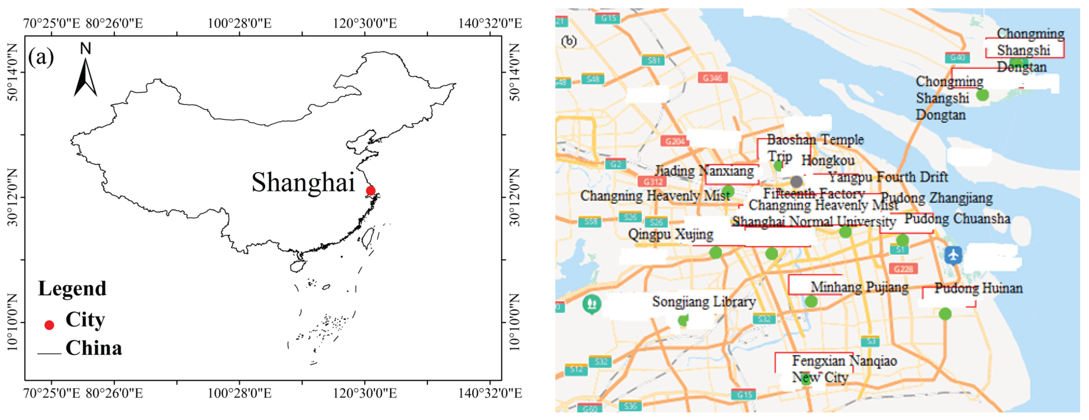
Figure 1. The geographical position of Shanghai city in China. (a) The location of Shanghai city in China; (b) the location of the monitoring sites in Shanghai city.
Toxics 11 00051 g001
Figure 2. Schematic diagram of 2-level wavelet decomposition.
Toxics 11 00051 g002
Figure 3. Artificial neural network architecture for mean daily PM2.5 concentration forecasting.
Toxics 11 00051 g003
Figure 4. Model structure of wavelet artificial neural network for mean daily PM2.5 concentration forecasting.
Toxics 11 00051 g004
Figure 5. The mean daily and annual variations of the original PM2.5 concentration data during the study period 2014–2020. (a) Daily PM2.5 concentration data, (b) annual PM2.5 concentration in the study area.
Toxics 11 00051 g005
Figure 6. Relevance between daily PM2.5 (t + 1) and input factors. (a) Correlation coefficient between meteorological elements and PM2.5 (t + 1). (b) Correlation coefficient between meteorological elements, PM2.5 (t) and PM2.5 (t + 1).
Toxics 11 00051 g006
Figure 7. Correlation between CA2, CD1 and CD2 for distinct wavelet functions (mother wavelets) in Shanghai during the testing phase; (a) wavelet Daubechies (db) and symlets (sym); (b) wavelet coiflets (coif) and biorthogonal wavelets (bior). Bior6.8 is a biorthogonal wavelet with an even symmetric high-pass decomposition filter.
Toxics 11 00051 g007
Figure 8. Performance comparison of different ANN and WANN structures and training algorithms in Shanghai during the testing phase. The training algorithms include trainbr (br), trainlm (lm), traingdx (gdx), traingd (gd), traingdm (gdm), trainrp (rp), traincgp (cgp), traincgf (cgf), traincgb (cgb), trainscg (scg), trainbfg (bfg), and trainoss (oss). (a) Performance of different nodes in hidden layer for ANN and WANN. (b) Performance of different training algorithms for ANN and WANN.
Toxics 11 00051 g008
Figure 9. Comparison between various activation functions for ANN and WANN in Shanghai during the training, verification and predicting phase. (a) RMSE for ANN, transfer functions include tansig(T), purelin(PU), logsig(L), and poslin(PO); (b) RMSE for WANN.
Toxics 11 00051 g009
Figure 10. The forecasting outcomes and scatter plots with the ANN models in the testing stage. (a) The predicted versus observed PM2.5 concentration, (b) scatter plots.
Toxics 11 00051 g010
Figure 11. The forecasting outcomes and scatter plots with the WANN models in the testing stage. (a) The predicted versus observed PM2.5 concentration, (b) scatter plots.
Toxics 11 00051 g011
Table 1. The list of the monitoring stations used in this study in Shanghai city.
Monitoring SitesMonitoring Sites
Jinshan New CityMinhang Pujiang
Chongming Shangshi DongtanQingpu Xujing
Chongming Shangshi DongtanShanghai Normal University
Yangpu Fourth DriftPudong Zhangjiang
Fifteenth FactoryBaoshan Temple Trip
Jing’an Monitoring StationFengxian Nanqiao New City
Pudong HuinanJiading Nanxiang
PutuoSongjiang Library
Pudong ChuanshaChangning Heavenly Mist
Pudong New Area Monitoring StationHongkou
Table 2. Sets of input factors that were tested with the ANN and WANN models for the predicting of next-day PM2.5 concentrations in Shanghai.
Model IDInput VariablesStructure
ANN1


ANN2
P (t), EWV (t), MAP (t), MWV (t), MAT (t), MWP (t), MRH (t), SH (t), MINAP (t), MINAT (t), MAXAP (t), MAXAT (t), MAXWV (t), MINRH (t), PM2.5 (t), PM2.5 (t − 1), PM2.5 (t − 2)
MINAT(t), MINAP(t), MAXAT(t), PM2.5 (t), PM2.5 (t − 1)
17:15:1


5:19:1
ANN3MINAT(t), PM2.5 (t)2:19:1
ANN4PM2.5 (t)1:21:1
WANN1P (t), EWV (t), MAP (t), MWV (t), MAT (t), MWP (t), MRH (t), SH (t), MINAP (t), MINAT (t), MAXAP (t), MAXAT (t), MAXWV (t), MINRH (t), PM2.5 (t), PM2.5 (t − 1), PM2.5 (t − 2)51:20:1
WANN2MINAT(t), MINAP(t), MAXAT(t), PM2.5 (t), PM2.5 (t − 1)15:20:1
WANN3MINAT(t), PM2.5 (t)6:17:1
WANN4PM2.5 (t)3:19:1
Table 3. Comparison of the performance statistics using different models.
ModelRRMSE (μg/m3)MAE (μg/m3)
TrainingVerificationPredictingTrainingVerificationPredictingTrainingVerificationPredicting
ANN10.70610.68300.561820.784117.000624.240715.082513.126217.7867
ANN20.62710.62580.473122.855918.199225.909216.334714.112518.9660
ANN30.59470.58310.445423.588318.708826.450416.912814.570719.2679
ANN40.57590.54500.424423.984718.976826.711717.219614.785619.7467
WANN10.94160.89690.93169.88249.785010.65807.11536.88277.6918
WANN20.90750.84240.883012.324311.923113.72288.45198.18259.1533
WANN30.79520.68600.721317.783616.146620.233212.533111.173314.6255
WANN40.73800.64040.704319.790317.058120.710613.531111.564314.7616
Table 4. The difference between existing PM2.5 prediction models and our model.
ModelAreaR2RERMSEMAEReference
ANNAhvaz, Iran0.740.9150746.44 [45]
ANNDelhi, India0.860.451 [55]
ANNAddis Ababa, Ethiopia0.9430.1203415.6610.27[56]
SVRNottingham, United Kingdom0.887820.122242.453151.29443[57]
XGBoostChina0.80.3638526.3415.58[58]
RNNSeoul metropolitan, Korea 0.31 8.4[59]
LSTMTianjin, China0.940.430513.068.61[60]
CNNBeijing, China0.72250.5884340.8325.32[61]
EMD-GRUBeijing, China0.97060.1480911.3726.532[62]
CNN-LSTMBeijing, China0.9215730.151824.228714.63446[63]
3D CNN-GRUTehran, Iran0.780.277816.44 8.89[64]
MCD-ESN-PSOfour cities, China0.98010.01671.180.88[65]
CNN-GBMShanghai, China0.850.0798210.02 [66]
iDeepAirShanghai, China 0.222715.58712.373[67]
GA-SVMShaanxi, China 0.1877312.110.07 [68]
WANNShanghai, China0.86790.136310.6587.6918This article
Disclaimer/Publisher’s Note: The statements, opinions and data contained in all publications are solely those of the individual author(s) and contributor(s) and not of MDPI and/or the editor(s). MDPI and/or the editor(s) disclaim responsibility for any injury to people or property resulting from any ideas, methods, instructions or products referred to in the content.