
Deep Learning-Based Indoor Air Quality Forecasting Framework for Indoor Subway Station Platforms


Abstract
:1. Introduction
2. Background and Literature Review
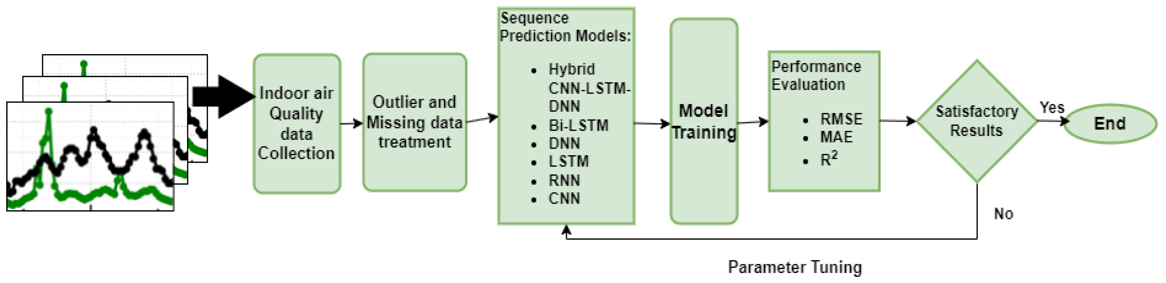
3. Hybrid CNN-LSTM Framework for Forecasting Indoor Subway Air Quality
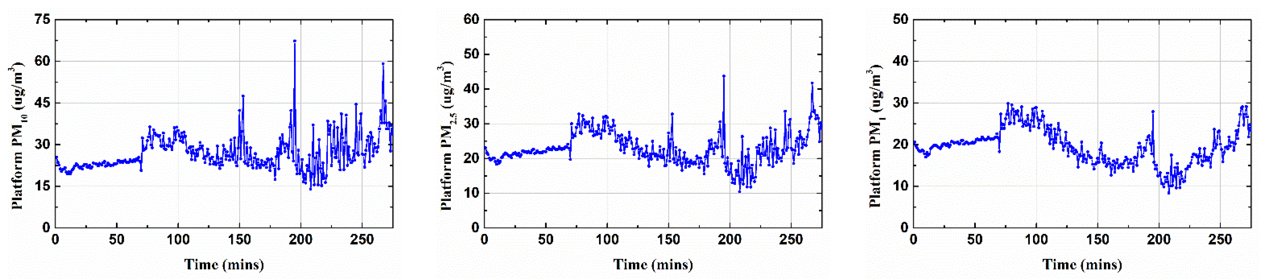
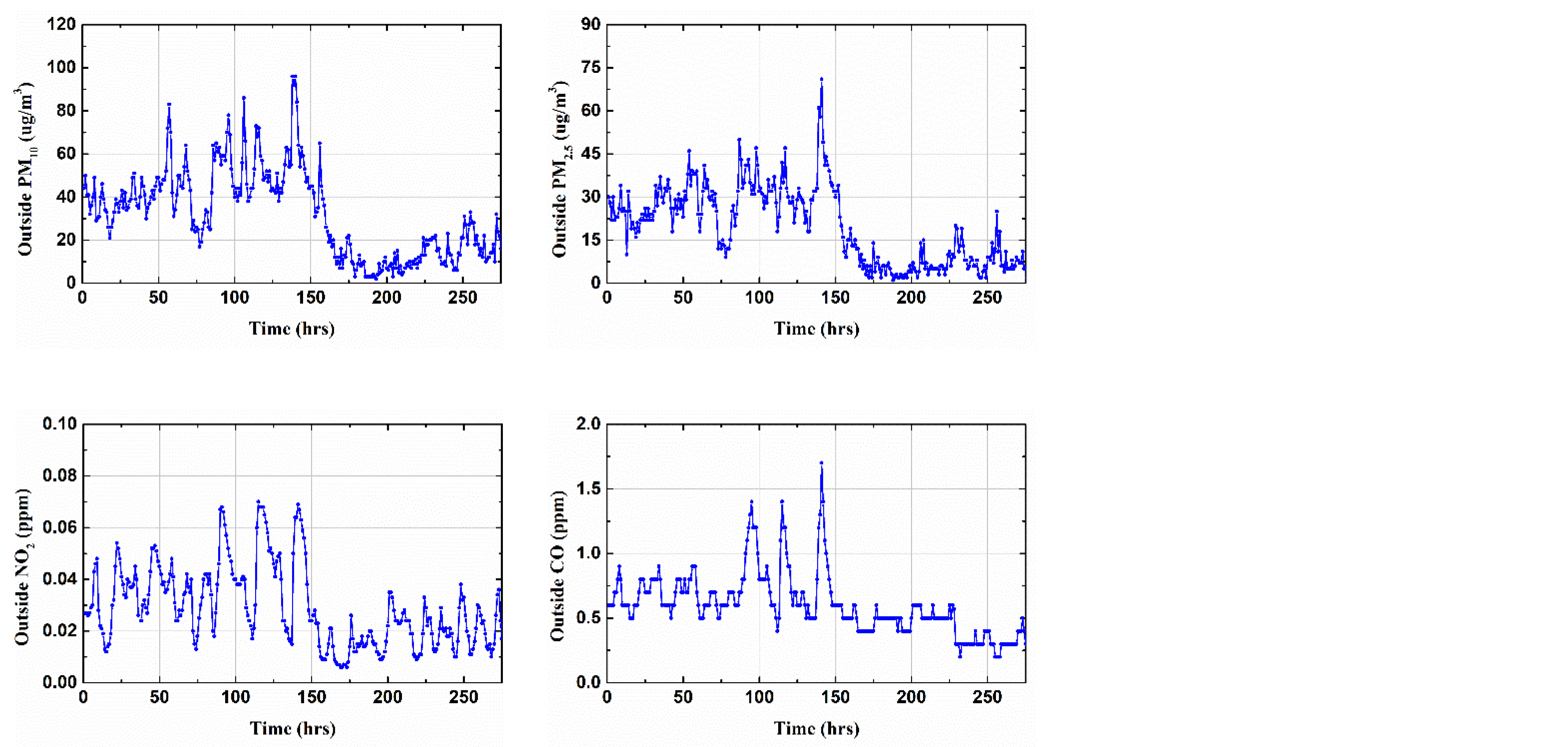
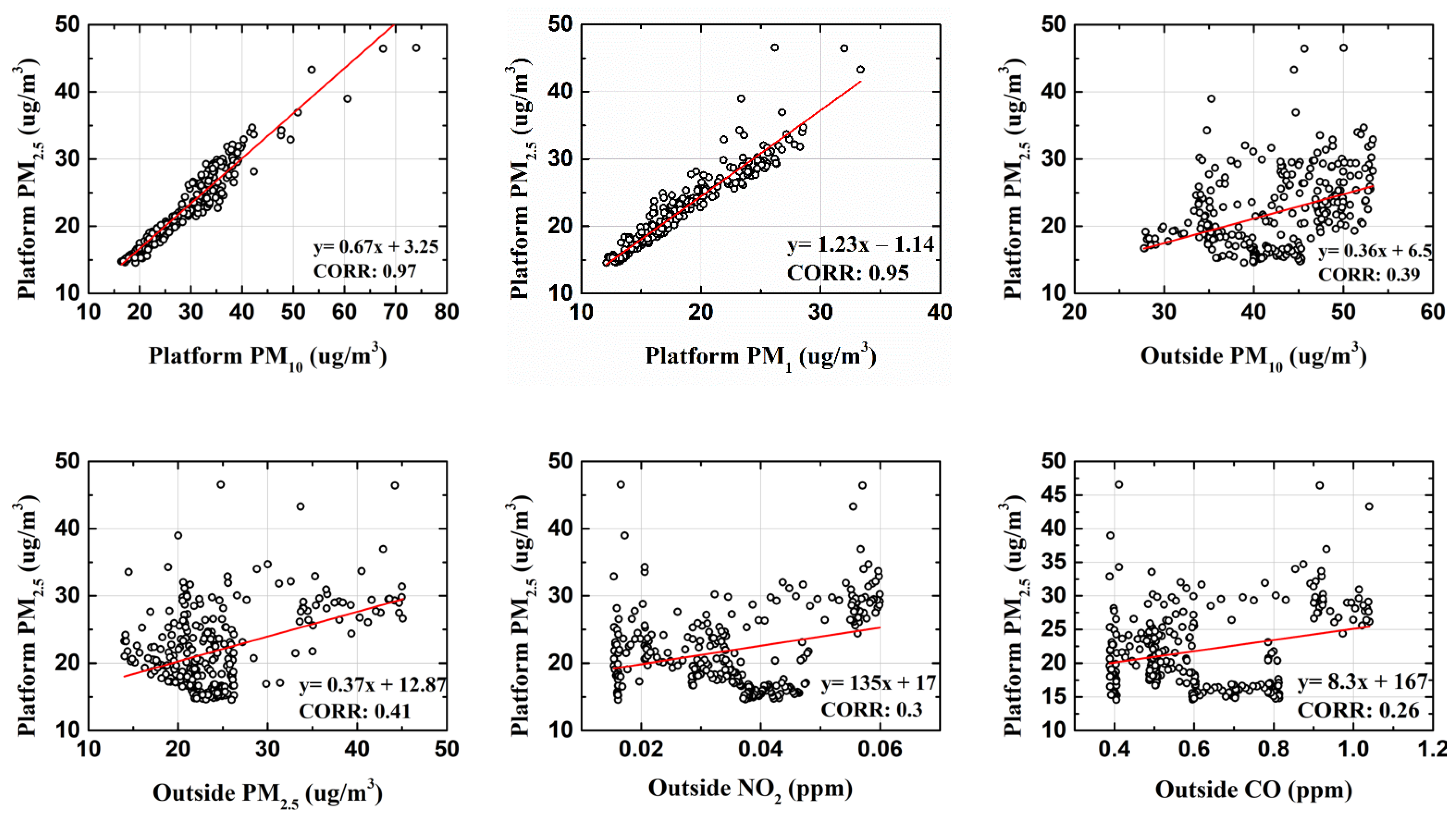
3.1. Data and Preliminary Information
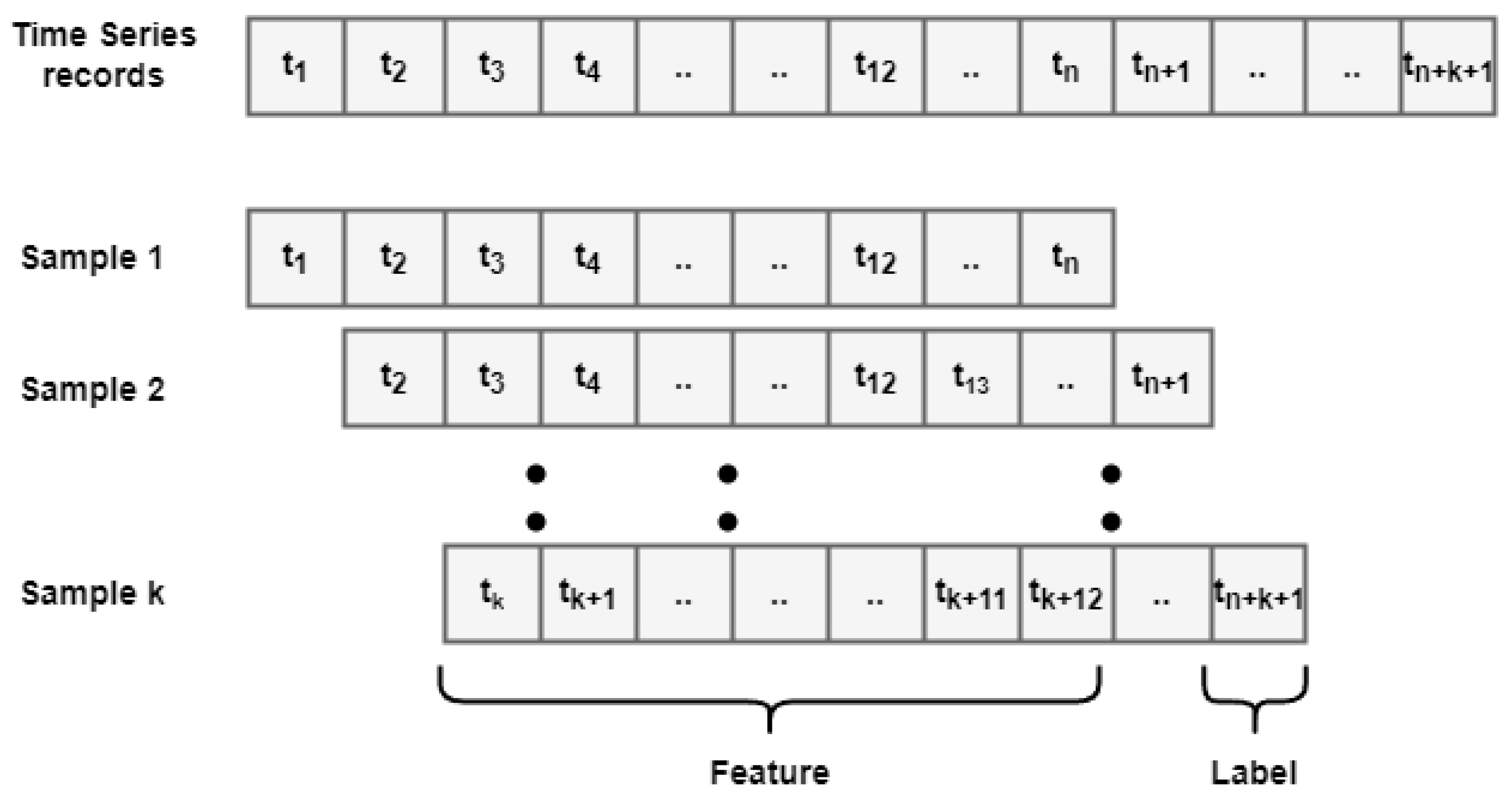
3.2. Preprocessing for Hybrid Deep Learning Framework
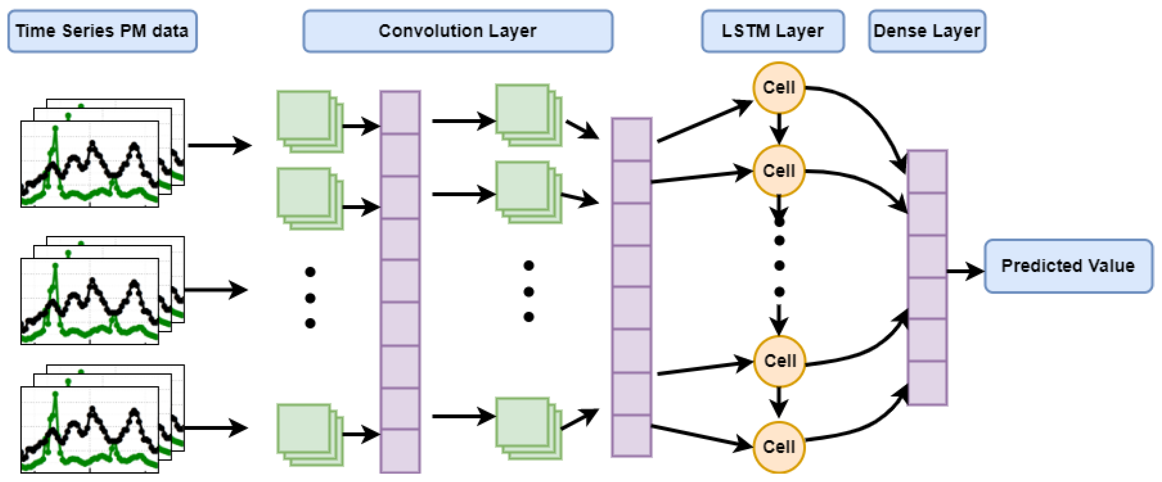
3.3. Proposed Hybrid Deep Learning Framework
3.4. Comparisons with Existing Deep Learning Models
3.4.1. LSTM and Bidirectional LSTM
3.4.2. DNN and CNN
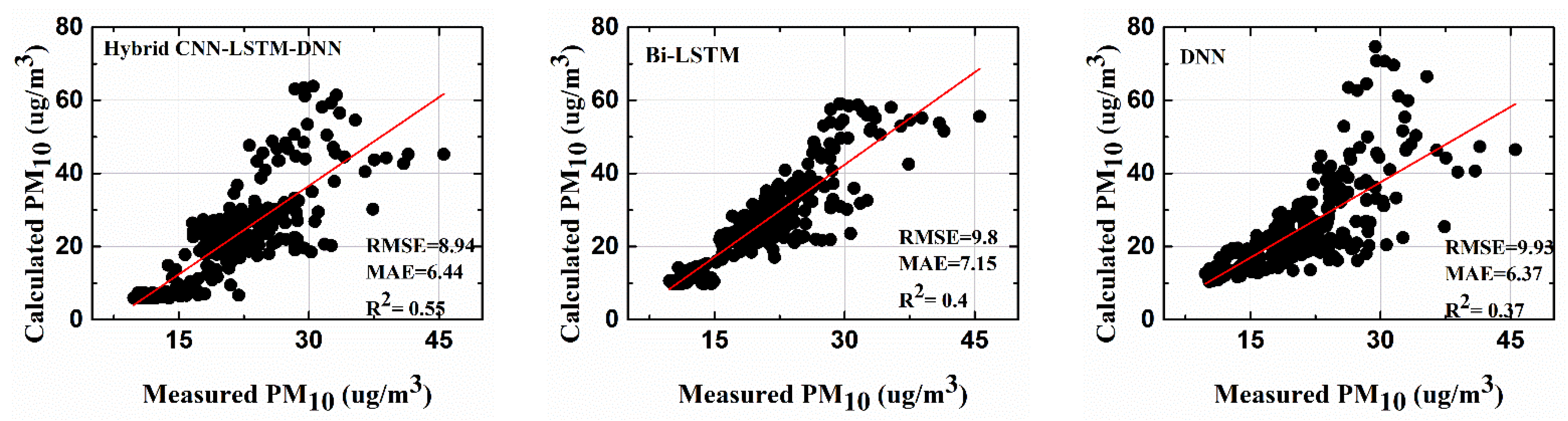
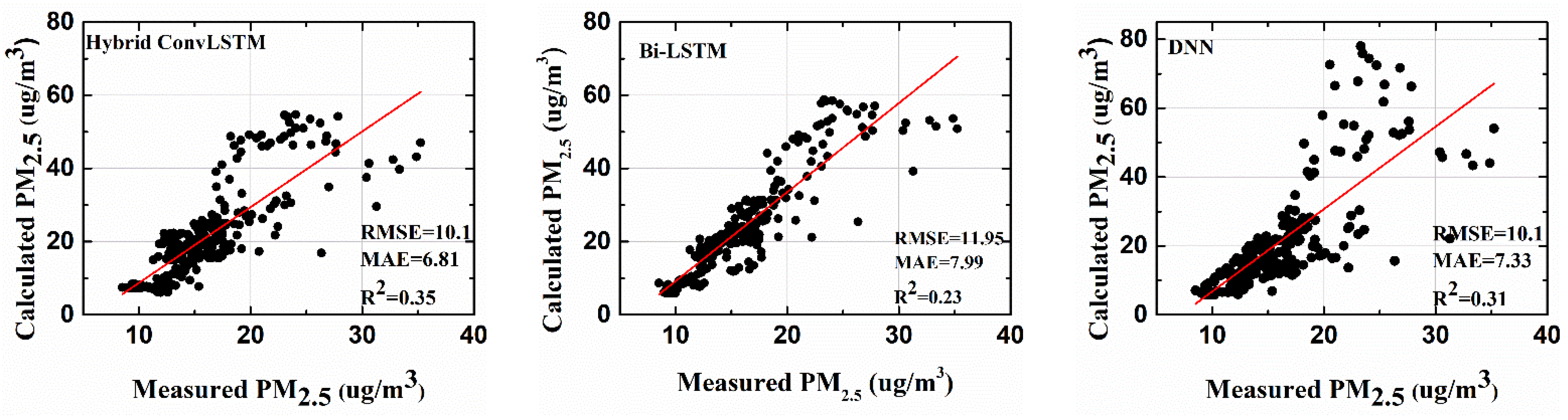
4. Indoor Air Quality Forecasting and Comparison Analysis
5. Conclusions
Author Contributions
Funding
Institutional Review Board Statement
Informed Consent Statement
Data Availability Statement
Conflicts of Interest
References
- Son, Y.S.; Oh, Y.H.; Choi, I.Y.; Dinh, T.V.; Chung, S.G.; Lee, J.H.; Park, D.; Kim, J.C. Development of a Magnetic Hybrid Filter to Reduce PM10 in a Subway Platform. J. Hazard. Mater. 2019, 368, 197–203. [Google Scholar] [CrossRef] [PubMed]
- Park, Y.; Choi, Y.; Kim, K.; Yoo, J.K. Machine Learning Approach for Study on Subway Passenger Flow. Sci. Rep. 2022, 12, 1–20. [Google Scholar] [CrossRef] [PubMed]
- Tariq, S.; Loy-Benitez, J.; Nam, K.J.; Lee, G.; Kim, M.J.; Park, D.S.; Yoo, C.K. Transfer Learning Driven Sequential Forecasting and Ventilation Control of PM2.5 Associated Health Risk Levels in Underground Public Facilities. J. Hazard. Mater. 2020, 406, 124753. [Google Scholar] [CrossRef] [PubMed]
- Rounce, P.; Tsolakis, A.; York, A.P.E. Speciation of Particulate Matter and Hydrocarbon Emissions from Biodiesel Combustion and Its Reduction by Aftertreatment. Fuel 2012, 96, 90–99. [Google Scholar] [CrossRef]
- United Nations Environment Programme (UNEP). Summary: Air Pollution in Asia and the Pacific: Science-Based Solutions Identifies; United Nations Environment Programme: Bangkok, Thailand, 2019. [Google Scholar]
- Chen, Z.; Cui, L.; Cui, X.; Li, X.; Yu, K.; Yue, K.; Dai, Z.; Zhou, J.; Jia, G.; Zhang, J. The Association between High Ambient Air Pollution Exposure and Respiratory Health of Young Children: A Cross Sectional Study in Jinan, China. Sci. Total Environ. 2018, 656, 740–749. [Google Scholar] [CrossRef] [PubMed]
- Li, X.; Zhang, X.; Zhang, Z.; Han, L.; Gong, D.; Li, J.; Wang, T.; Wang, Y.; Gao, S.; Duan, H.; et al. Air Pollution Exposure and Immunological and Systemic Inflammatory Alterations among Schoolchildren in China. Sci. Total Environ. 2018, 657, 1304–1310. [Google Scholar] [CrossRef] [PubMed]
- Ngoc, L.T.N.; Lee, Y.; Chun, H.-S.; Moon, J.-Y.; Choi, J.S.; Park, D.; Lee, Y.-C. Correlation of α/γ-Fe2O3 Nanoparticles with the Toxicity of Particulate Matter Originating from Subway Tunnels in Seoul Stations, Korea. J. Hazard. Mater. 2019, 382, 121175. [Google Scholar] [CrossRef]
- Li, T.T.; Bai, Y.H.; Liu, Z.R.; Li, J.L. In-Train Air Quality Assessment of the Railway Transit System in Beijing: A Note. Transp. Res. Part D Transp. Environ. 2007, 12, 64–67. [Google Scholar] [CrossRef]
- Van Ryswyk, K.; Anastasopolos, A.T.; Evans, G.; Sun, L.; Sabaliauskas, K.; Kulka, R.; Wallace, L.; Weichenthal, S. Metro Commuter Exposures to Particulate Air Pollution and PM2.5-Associated Elements in Three Canadian Cities: The Urban Transportation Exposure Study. Environ. Sci. Technol. 2017, 51, 5713–5720. [Google Scholar] [CrossRef]
- Park, D.U.; Ha, K.C. Characteristics of PM10, PM2.5, CO2 and CO Monitored in Interiors and Platforms of Subway Train in Seoul, Korea. Environ. Int. 2008, 34, 629–634. [Google Scholar] [CrossRef]
- Johansson, C.; Johansson, P.Å. Particulate Matter in the Underground of Stockholm. Atmospheric Environ. 2003, 37, 3–9. [Google Scholar] [CrossRef]
- Adams, H.S.; Nieuwenhuijsen, M.J.; Colvile, R.N. Determinants of Fine Particle (PM2.5) Personal Exposure Levels in Transport Microenvironments, London, UK. Atmospheric Environ. 2001, 35, 4557–4566. [Google Scholar] [CrossRef]
- Liu, H.; Wang, X.; Zhang, J.; He, K.; Wu, Y.; Xu, J. Emission Controls and Changes in Air Quality in Guangzhou during the Asian Games. Atmospheric Environ. 2012, 76, 81–93. [Google Scholar] [CrossRef]
- The World Bank Group. The World Bank Annual Report 2017: End Extreme Poverty, Boost Shared Prosperity; World Bank: Washington, DC, USA, 2017; pp. 1–87. [Google Scholar]
- Marsik, T.; Johnson, R. HVAC Air-Quality Model and Its Use to Test a PM2.5 Control Strategy. Build. Environ. 2008, 43, 1850–1857. [Google Scholar] [CrossRef]
- Kim, M.J.; Braatz, R.D.; Kim, J.T.; Yoo, C.K. Indoor Air Quality Control for Improving Passenger Health in Subway Platforms Using an Outdoor air Quality Dependent Ventilation System. Build. Environ. 2015, 92, 407–417. [Google Scholar] [CrossRef]
- Wang, F.; Meng, D.; Li, X.; Tan, J. Indoor-Outdoor Relationships of PM2.5 in Four Residential Dwellings in Winter in the Yangtze River Delta, China. Environ. Pollut. 2016, 215, 280–289. [Google Scholar] [CrossRef]
- Shrestha, P.M.; Humphrey, J.L.; Carlton, E.J.; Adgate, J.L.; Barton, K.E.; Root, E.D.; Miller, S.L. Impact of Outdoor Air Pollution on Indoor Air Quality in Low-Income Homes during Wildfire Seasons. Int. J. Environ. Res. Public Health 2019, 16, 3535. [Google Scholar] [CrossRef]
- Hodzic, A.; Madronich, S.; Bonn, B.; Massie, S.; Menut, L.; Wiedinmyer, C. Wildfire Particulate Matter in Europe during Summer 2003: Meso-Scale Modeling of Smoke Emissions, Transport and Radiative Effects. Atmospheric Chem. Phys. 2007, 7, 4043–4064. [Google Scholar] [CrossRef]
- McMeeking, G.R.; Kreidenweis, S.M.; Lunden, M.; Carrillo, J.; Carrico, C.M.; Lee, T.; Herckes, P.; Engling, G.; Day, D.E.; Hand, J.; et al. Smoke-Impacted Regional Haze in California during the Summer of 2002. Agric. For. Meteorol. 2006, 137, 25–42. [Google Scholar] [CrossRef]
- Wang, Y.; Liu, C.G.; Wang, Q.; Qin, Q.; Ren, H.; Cao, J. Impacts of Natural and Socioeconomic Factors on PM2.5 from 2014 to 2017. J. Environ. Manag. 2021, 284, 112071. [Google Scholar] [CrossRef]
- Tariq, S.; Loy-Benitez, J.; Nam, K.J.; Heo, S.; Yoo, C.K. Energy-Efficient Time-Delay Compensated Ventilation Control System for Sustainable Subway Air Quality Management under Various Outdoor Conditions. Build. Environ. 2020, 174, 106775. [Google Scholar] [CrossRef]
- Yang, Z.; Wang, J. A New Air Quality Monitoring and Early Warning System: Air Quality Assessment and Air Pollutant Concentration Prediction. Environ. Res. 2017, 158, 105–117. [Google Scholar] [CrossRef] [PubMed]
- Park, S.; Kim, M.; Kim, M.; Namgung, H.G.; Kim, K.T.; Cho, K.H.; Kwon, S.B. Predicting PM10 Concentration in Seoul Metropolitan Subway Stations Using Artificial Neural Network (ANN). J. Hazard. Mater. 2018, 341, 75–82. [Google Scholar] [CrossRef] [PubMed]
- Cashikar, A.; Li, J.; Biswas, P. Particulate Matter Sensors Mounted on a Robot for Environmental Aerosol Measurements. J. Environ. Eng. 2019, 145, 04019057. [Google Scholar] [CrossRef]
- Srinivas, C.V.; Subramanian, V.; Kumar, A.; Usha, P.; Sujatha, N.; Singh, A.B.; Rakesh, P.T.; Baskaran, R.; Venkatraman, B. Modeling of Atmospheric Dispersion of Sodium Fire Aerosols for Environmental Impact Analysis during Accidental Leaks. J. Aerosol Sci. 2019, 137, 105432. [Google Scholar] [CrossRef]
- Nsir, K.; Sartelet, K.; Bresson, R.; Genon, L.M. Three-Dimensional Computational Fluid Dynamics Modelling of Sodium Oxide Aerosol Atmospheric Dispersion from Indoor Sodium Fire. J. Aerosol Sci. 2019, 137, 105433. [Google Scholar] [CrossRef]
- Periáñez, R.; Thiessen, K.M.; Chouhan, S.L.; Mancini, F.; Navarro, E.; Sdouz, G.; Trifunović, D. Mid-Range Atmospheric Dispersion Modelling. Intercomparison of Simple Models in EMRAS-2 Project. J. Environ. Radioact. 2016, 162, 225–234. [Google Scholar] [CrossRef] [PubMed]
- Jian, L.; Zhao, Y.; Zhu, Y.-P.; Zhang, M.-B.; Bertolatti, D. An Application of ARIMA Model to Predict Submicron Particle Concentrations from Meteorological Factors at a Busy Roadside in Hangzhou, China. Sci. Total Environ. 2012, 426, 336–345. [Google Scholar] [CrossRef] [PubMed]
- Slini, T.; Karatzas, K.; Moussiopoulos, N. Statistical Analysis of Environmental Data as the Basis of Forecasting: An Air Quality Application. Sci. Total Environ. 2002, 288, 227–237. [Google Scholar] [CrossRef]
- Suleiman, A.; Tight, M.R.; Quinn, A.D. Applying Machine Learning Methods in Managing Urban Concentrations of Traffic-Related Particulate Matter (PM10 and PM2.5). Atmos. Pollut. Res. 2018, 10, 134–144. [Google Scholar] [CrossRef]
- Osowski, S.; Garanty, K. Forecasting of the Daily Meteorological Pollution Using Wavelets and Support Vector Machine. Eng. Appl. Artif. Intell. 2007, 20, 745–755. [Google Scholar] [CrossRef]
- Chang, H.; Lee, Y.; Yoon, B.; Baek, S. Dynamic Near-Term Traffic Flow Prediction: System-Oriented Approach Based on Past Experiences. IET Intell. Transp. Syst. 2012, 6, 292–305. [Google Scholar] [CrossRef]
- Neagu, C.D.; Avouris, N.; Kalapanidas, E.; Palade, V. Neural and Neuro-Fuzzy Integration in a Knowledge-Based System for Air Quality Prediction. Appl. Intell. 2002, 17, 141–169. [Google Scholar] [CrossRef]
- Alimissis, A.; Philippopoulos, K.; Tzanis, C.G.; Deligiorgi, D. Spatial Estimation of Urban Air Pollution with the Use of Artificial Neural Network Models. Atmos. Environ. 2018, 191, 205–213. [Google Scholar] [CrossRef]
- Goulier, L.; Paas, B.; Ehrnsperger, L.; Klemm, O. Modelling of Urban Air Pollutant Concentrations with Artificial Neural Networks Using Novel Input Variables. Int. J. Environ. Res. Public Health 2020, 17, 2025. [Google Scholar] [CrossRef]
- Elbayoumi, M.; Ramli, N.A.; Yusof, N.F.F.M. Development and Comparison of Regression Models and Feedforward Backpropagation Neural Network Models to Predict Seasonal Indoor PM2.5–10 and PM2.5 Concentrations in Naturally Ventilated Schools. Atmospheric Pollut. Res. 2015, 6, 1013–1023. [Google Scholar] [CrossRef]
- Ayturan, Y.A.; Ayturan, Z.C.; Altun, H.O. Air Pollution Modelling with Deep Learning: A Review. Int. J. Enironmental Pollut. Environ. Model. 2018, 1, 58. [Google Scholar]
- Bakht, A.; Lee, H. Deep Learning Framework for Spatial Crowdedness Estimation and Comparison Analysis with Machine Learning. J. Korean Inst. Intell. Syst. 2022, 32, 76–85. [Google Scholar] [CrossRef]
- Bakht, A.; Nawaz, A.; Lee, M.; Lee, H. Hybrid Multi-Stream Deep Learning-Based Nutrient Estimation Framework in Biological Wastewater Treatement. J. Korean Inst. Intell. Syst. 2022, 32, 209–217. [Google Scholar]
- Loy-Benitez, J.; Li, Q.; Ifaei, P.; Nam, K.; Heo, S.K.; Yoo, C. A Dynamic Gain-Scheduled Ventilation Control System for a Subway Station Based on Outdoor Air Quality Conditions. Build. Environ. 2018, 144, 159–170. [Google Scholar] [CrossRef]
- Man, Y.; Hu, Y.; Ren, J. Forecasting COD Load in Municipal Sewage Based on ARMA and VAR Algorithms. Resour. Conserv. Recycl. 2019, 144, 56–64. [Google Scholar] [CrossRef]
- Qi, Y.; Li, Q.; Karimian, H.; Liu, D. A Hybrid Model for Spatiotemporal Forecasting of PM2.5 Based on Graph Convolutional Neural Network and Long Short-Term Memory. Sci. Total Environ. 2019, 664, 1–10. [Google Scholar] [CrossRef] [PubMed]
- Du, S.; Li, T.; Yang, Y.; Horng, S.J. Deep Air Quality Forecasting Using Hybrid Deep Learning Framework. IEEE Trans. Knowl. Data Eng. 2021, 33, 2412–2424. [Google Scholar] [CrossRef]
- Rahmadani, F.; Lee, H. Hybrid Deep Learning-Based Epidemic Prediction Framework of COVID-19: South Korea Case. Appl. Sci. 2020, 10, 8539. [Google Scholar] [CrossRef]
- Lee, H.; Han, S.-Y.; Park, K.; Lee, H.; Kwon, T. Real-Time Hybrid Deep Learning-Based Train Running Safety Prediction Framework of Railway Vehicle. Machines 2021, 9, 130. [Google Scholar] [CrossRef]
- Yang, D.; Wang, J.; Yan, X.; Liu, H. Subway Air Quality Modeling Using Improved Deep Learning Framework. Process Saf. Environ. Prot. 2022, 163, 487–497. [Google Scholar] [CrossRef]
- Hochreiter, S.; Schmidhuber, J. Long Short-Term Memory. Neural Comput. 1997, 9, 1735–1780. [Google Scholar] [CrossRef]
- Zhou, Y.; Chang, F.-J.; Chang, L.-C.; Kao, I.-F.; Wang, Y.-S. Explore a Deep Learning Multi-Output Neural Network for Regional Multi-Step-Ahead Air Quality Forecasts. J. Clean. Prod. 2018, 209, 134–145. [Google Scholar] [CrossRef]
- Wu, Q.; Lin, H. A Novel Optimal-Hybrid Model for Daily Air Quality Index Prediction Considering Air Pollutant Factors. Sci. Total Environ. 2019, 683, 808–821. [Google Scholar] [CrossRef]
- Graves, A.; Schmidhuber, J. Framewise Phoneme Classification with Bidirectional LSTM and Other Neural Network Architectures. Neural Netw. 2005, 18, 602–610. [Google Scholar] [CrossRef]


| Item | |||||||
|---|---|---|---|---|---|---|---|
| (µg/m3) | (µg/m3) | (µg/m3) | (µg/m3) | (µg/m3) | (ppm) | (ppm) | |
| Minimum | 1.93 | 1.89 | 1.27 | 1.98 | 0.90 | 0.01 | 0.19 |
| Maximum | 260.24 | 145.97 | 126.36 | 184.64 | 114.83 | 0.08 | 1.70 |
| Mean | 32.95 | 26.95 | 22.37 | 43.86 | 24.42 | 0.03 | 0.62 |
| Standard Deviation | 23.51 | 20.90 | 18.54 | 26.65 | 18.13 | 0.01 | 0.24 |
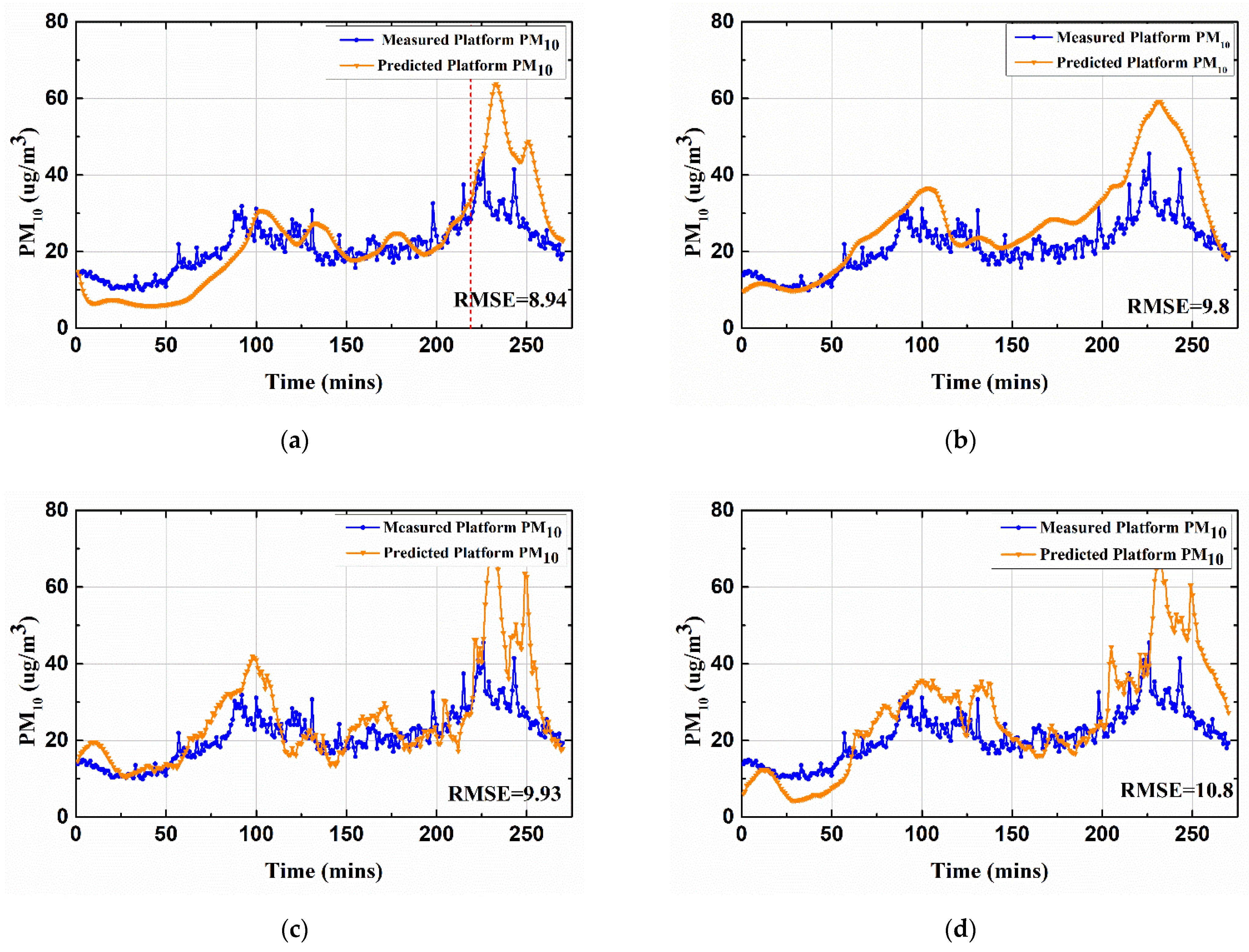
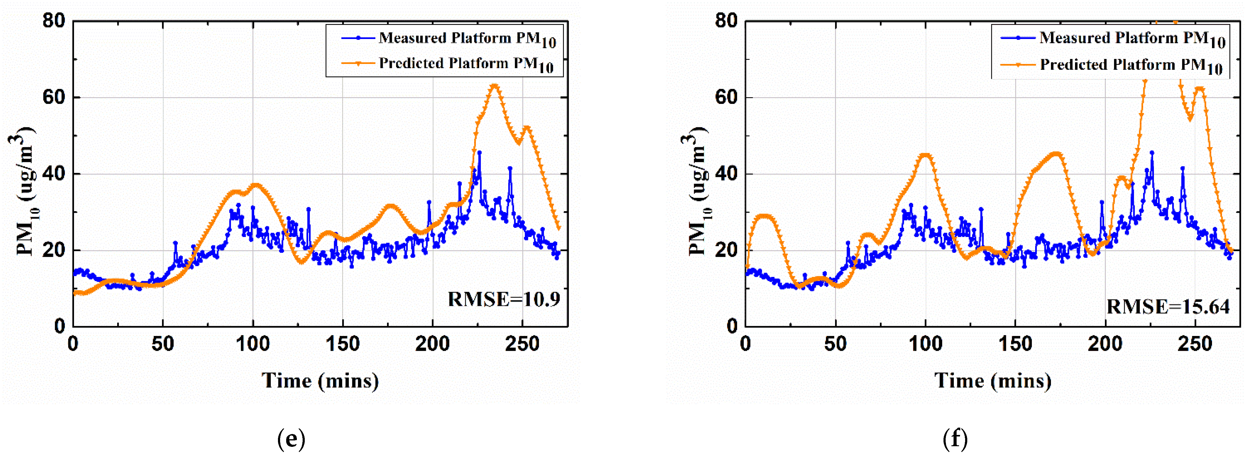
| Comparison Model | ||||||
|---|---|---|---|---|---|---|
| RMSE | MAE | R2 | RMSE | MAE | R2 | |
| Hybrid Deep learning framework (proposed) | 8.94 | 6.44 | 0.55 | 10.1 | 6.81 | 0.35 |
| BILSTM | 9.8 | 7.15 | 0.4 | 11.95 | 7.99 | 0.23 |
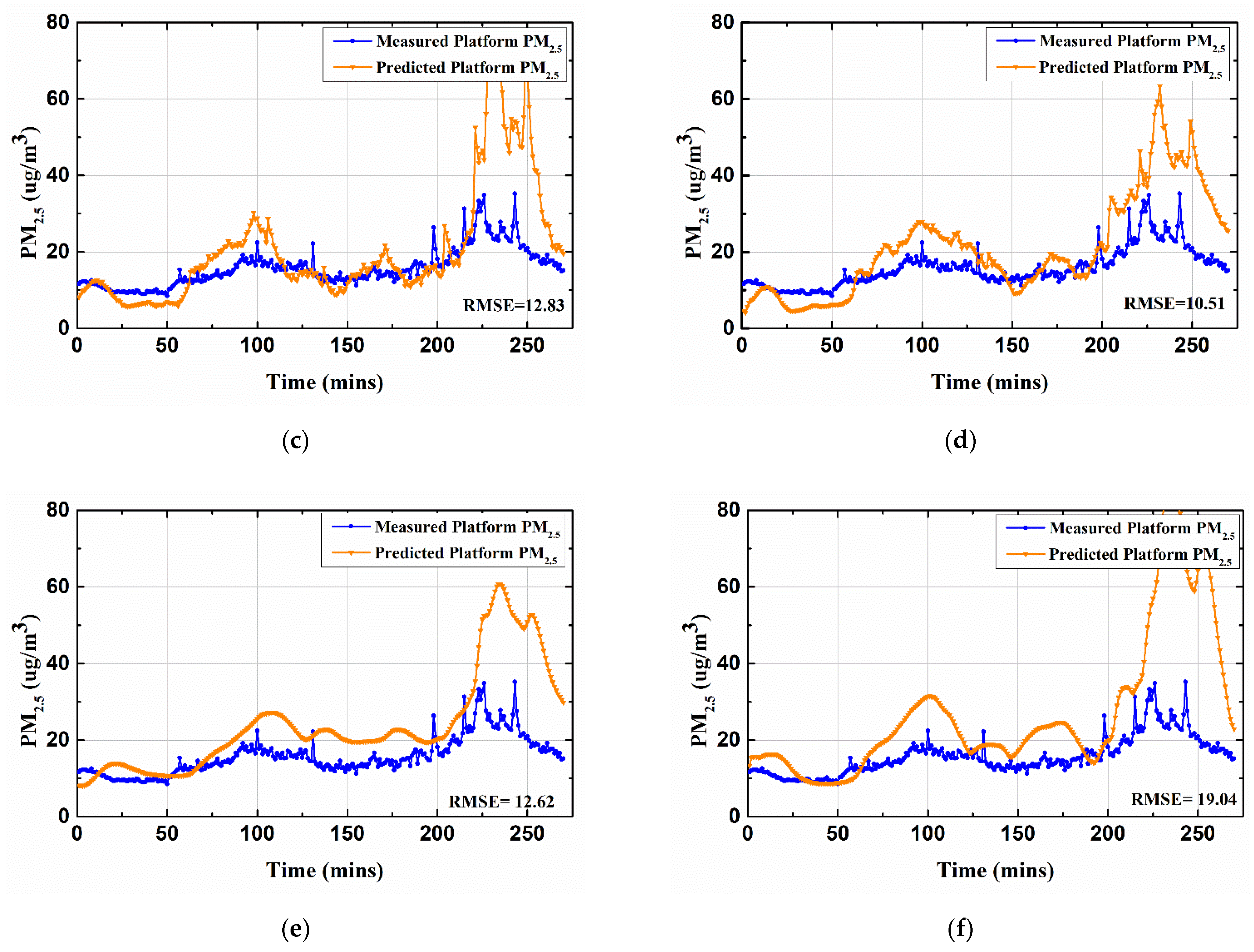
| DNN | 9.93 | 6.37 | 0.37 | 12.83 | 7.33 | 0.31 |
| LSTM | 10.8 | 7.89 | 0.41 | 10.51 | 7.55 | 0.34 |
| RNN | 10.98 | 7.93 | 0.33 | 12.62 | 8.08 | 0.1 |
| CNN | 15.64 | 10.41 | 0.15 | 19.04 | 11.89 | 0 |
Publisher’s Note: MDPI stays neutral with regard to jurisdictional claims in published maps and institutional affiliations. |
© 2022 by the authors. Licensee MDPI, Basel, Switzerland. This article is an open access article distributed under the terms and conditions of the Creative Commons Attribution (CC BY) license (https://creativecommons.org/licenses/by/4.0/).
Share and Cite
Bakht, A.; Sharma, S.; Park, D.; Lee, H. Deep Learning-Based Indoor Air Quality Forecasting Framework for Indoor Subway Station Platforms. Toxics 2022, 10, 557. https://doi.org/10.3390/toxics10100557
Bakht A, Sharma S, Park D, Lee H. Deep Learning-Based Indoor Air Quality Forecasting Framework for Indoor Subway Station Platforms. Toxics. 2022; 10(10):557. https://doi.org/10.3390/toxics10100557
Chicago/Turabian StyleBakht, Ahtesham, Shambhavi Sharma, Duckshin Park, and Hyunsoo Lee. 2022. "Deep Learning-Based Indoor Air Quality Forecasting Framework for Indoor Subway Station Platforms" Toxics 10, no. 10: 557. https://doi.org/10.3390/toxics10100557
APA StyleBakht, A., Sharma, S., Park, D., & Lee, H. (2022). Deep Learning-Based Indoor Air Quality Forecasting Framework for Indoor Subway Station Platforms. Toxics, 10(10), 557. https://doi.org/10.3390/toxics10100557