Development of a Novel Fuzzy Hierarchical Location-Routing Optimization Model Considering Reliability

Abstract

Background: This paper discusses the optimization of a novel fuzzy hierarchical location-routing problem, taking into consideration reliability. The mathematical model presented aims to determine the optimal locations of production centers and warehouses, as well as the optimal routing of vehicles, in order to minimize total costs. Methods: Because of the uncertainty surrounding the demand and transportation cost parameters, a fuzzy programming method was employed to control the model. To solve the mathematical model, both GA and PSO algorithms were used. Results: The results show that as the uncertainty rate increases, the total costs also increase. Additionally, the results indicate that the maximum relative difference percentage between the solutions of the GA and PSO, and the optimal solutions are 0.587 and 0.792, respectively. On the other hand, analysis of numerical examples demonstrates that the Baron Solver is unable to solve large-scale numerical examples. Conclusions: By comparing the results of GA and PSO, it is observed that PSO was able to solve numerical examples in less time than GA, while GA obtained better results than PSO. Therefore, the TOPSIS method was used to rank the different solution methods, which resulted in GA being recognized as an effective algorithm with a utility weight of 0.972.

1. Introduction

The ever-increasing development of urbanization, industries, and especially support industries has resulted in the movement of people and goods becoming a problem with constantly increasing complexity. Urban growth has led to a higher demand in the transportation industry, which in turn has caused major cities and industries to face numerous issues such as traffic congestion, air pollution, long travel times for daily commutes, increased fuel consumption, and vehicle depreciation [1]. To address these traffic problems and the economic, social, and environmental challenges arising from them in big cities, manufacturing industries, and the service sector, a well-equipped and efficient transportation system is necessary. Transportation is a crucial sector of any country’s economy and one of the primary contributors to the cost of finished products [2]. One of the reasons why the vehicle routing problem (VRP) is considered a significant issue in combination optimization and has garnered the attention of many researchers is its practical application in the real world.

Today, many goods distribution companies use multiple warehouses for collecting and distributing goods. However, using a warehouse for distributing goods within the service area may not be economically viable [3]. In certain situations, direct services from the central warehouse to customers may not be possible. In such cases, service is provided through intermediate points, commonly known as urban distribution centers [4]. The Hierarchical Vehicle Routing Problem (HVRP) arises in two-echelon transportation systems, particularly in the field of urban logistics. In these systems, the cargo is transported to a main terminal and then sent to the final customers. The HVRP considers two echelons: the first involves delivering goods from production centers to warehouses, and the second involves delivering goods from warehouses to customers. To minimize the total routing cost at each echelon [2], a constraint on the number of vehicles is imposed. It is evident that the HVRP is an extension of the classical Vehicle Routing Problem (VRP) and, as a result, it is NP-Hard. Thus, finding the optimal solution in polynomial time is impossible. The complexity of this problem is further heightened by the presence of numerous input parameters, including the number of vehicles, customers, and routes [5,6].

In this paper, vehicle routing is not the only consideration; in addition to this decision, the location of potential centers is also of great importance. Therefore, strategic decisions such as determining the location of production centers and warehouses, as well as tactical decisions such as vehicle routing between production centers and warehouses, and between warehouses and customers, are made. The objective function of minimizing total costs is considered in order to achieve these decisions. Due to the lack of access to historical data, demand and transportation costs are considered as uncertainty parameters. Therefore, a fuzzy programming method is proposed to control the model, and Genetic Algorithm (GA) and Particle Swarm Optimization (PSO) are used to solve the model.

This paper is divided into six sections. The second section discusses the literature review. The third section presents a novel fuzzy hierarchical location-routing problem (FHLRP) and utilizes a fuzzy programming method to control the model. In the fourth section, problem-solving methods are presented, and an initial solution is designed for GA and PSO. The fifth section examines the results and includes various numerical examples. Additionally, the prioritization of solution methods is conducted using the TOPSIS method. Finally, the sixth section concludes with discussions on recommendations for future research.

2. Literature Review

Due to the importance of VRP and facility location, extensive research has been conducted over the past decades, resulting in various developments and solutions. For instance, Zhang et al. [7] proposed a VRP that aimed at minimizing both the total distance and CO2 gas emissions. They utilized a hybrid artificial bee colony algorithm to solve this problem. In another study, Ghahremani-Nahr et al. [8] presented a multi-objective model for the food bank network that simultaneously addressed the location-routing inventory and allocation issues. They employed NSGA II and MOGWO algorithms to solve this problem. Alinaghian and Shokouhi [9] developed a mathematical model to solve the multi-depot multi-compartment VRP. The objective function of their model focused on minimizing the number of vehicles and the distances traveled on all routes. To solve this model, they utilized a hybrid adaptive large neighborhood search. Additionally, Brandão [10] designed an open VRP that took into account time windows and employed an iterated local search algorithm to find a solution. Babaee Tirkolaee et al. [11] developed a multi-objective mixed-integer linear programming model for the two-echelon green capacity VRP, considering environmental issues and time window constraints for the perishable product delivery phase. Breunig et al. [12] introduced an algorithm for the two-echelon VRP and examined the results using an exact algorithm. Their goal in this model was to reduce the total vehicle routing costs. Yan et al. [13] dealt with making strategic and tactical decisions in the two-echelon VRP. They presented a model to reduce the costs of locating warehouses and distributing products through different vehicles in the first and second echelon.

Ji et al. [14] modeled an inventory VRP for perishable products with a time window constraint. Their goal was to minimize total costs with respect to uncertain demand. Del-laert et al. [15] investigated the multi-product two-echelon capacity VRP considering time windows. In this study, they presented an accurate method for optimal routing in the first and second echelons, and the results showed the high efficiency of their solution method. Du et al. [16] presented a new model for the two-echelon VRP in which a fleet of homogeneous vehicles is responsible for delivering products to customers. Huang et al. [17] presented a model for a two-echelon VRP in which the location decisions of intermediate warehouses and the optimal routing of vehicle transport are considered. They used a heuristic algorithm with a Hamiltonian graph to solve the problem. Zhou et al. [18] proposed a two-echelon VRP with simultaneous pickup and delivery as well as a soft time window. They used the Tabu search algorithm to find the optimal transport routing. Goli et al. [19] presented a new solution method for a two-echelon distribution system using electric vehicles considering the time window. In the first, the required products are sent from a central warehouse to the satellite stations, and in the second, these products are distributed to different customers. Nozari et al. [20] modeled a multi-depot VRP model where demand and transportation costs were considered as fuzzy numbers. They used a fuzzy robust method to control the model. Hajghani et al. [21] presented a two-echelon vehicle routing-location model under uncertainty, in which distribution center location decisions and vehicle routing decisions are made simultaneously. Zhou et al. [22] presented an exact algorithm for solving the two-echelon VRP for unmanned aircraft. In this model, several drones were responsible for providing services to customers. Jia et al. [23] addressed the optimization of VRP from multiple distribution centers called depots. This issue included determining the appropriate transportation route from warehouses to satellites and delivery from satellites to final customers. Du et al. [24] designed an energy-efficient collaborative delivery network for various express companies to provide fast delivery services to customers. They modeled a two-echelon capacitated VRP considering carbon emissions for rapid delivery network optimization. Sluijk et al. [25] studied the two-echelon VRP with stochastic demand, and they used an efficient algorithm to optimize the paths in the both of the first and the second echelons.

A review of the research literature shows that the models presented for the VRP mainly focus on location-routing-allocation decisions. This means that only one echelon is responsible for archiving the optimum route of the vehicle. However, considering the complexity of the VRP, this paper introduces a novel FHLRP that addresses vehicle routing and facility location at both echelons. This means that in each echelon, vehicle routing and facility location are considered simultaneously. Additionally, in all previous research, the reliability of facility location and vehicle routing has not been taken into account. Based on the literature review, the innovations of the paper can be summarized as follows:

• Designing a comprehensive model of FHLRP.
• Considering reliability in positioning-routing to increase customer satisfaction.
• Using the fuzzy programming method to control the demand and transportation cost parameters due to the lack of access to historical data.

3. Definition of the Problem

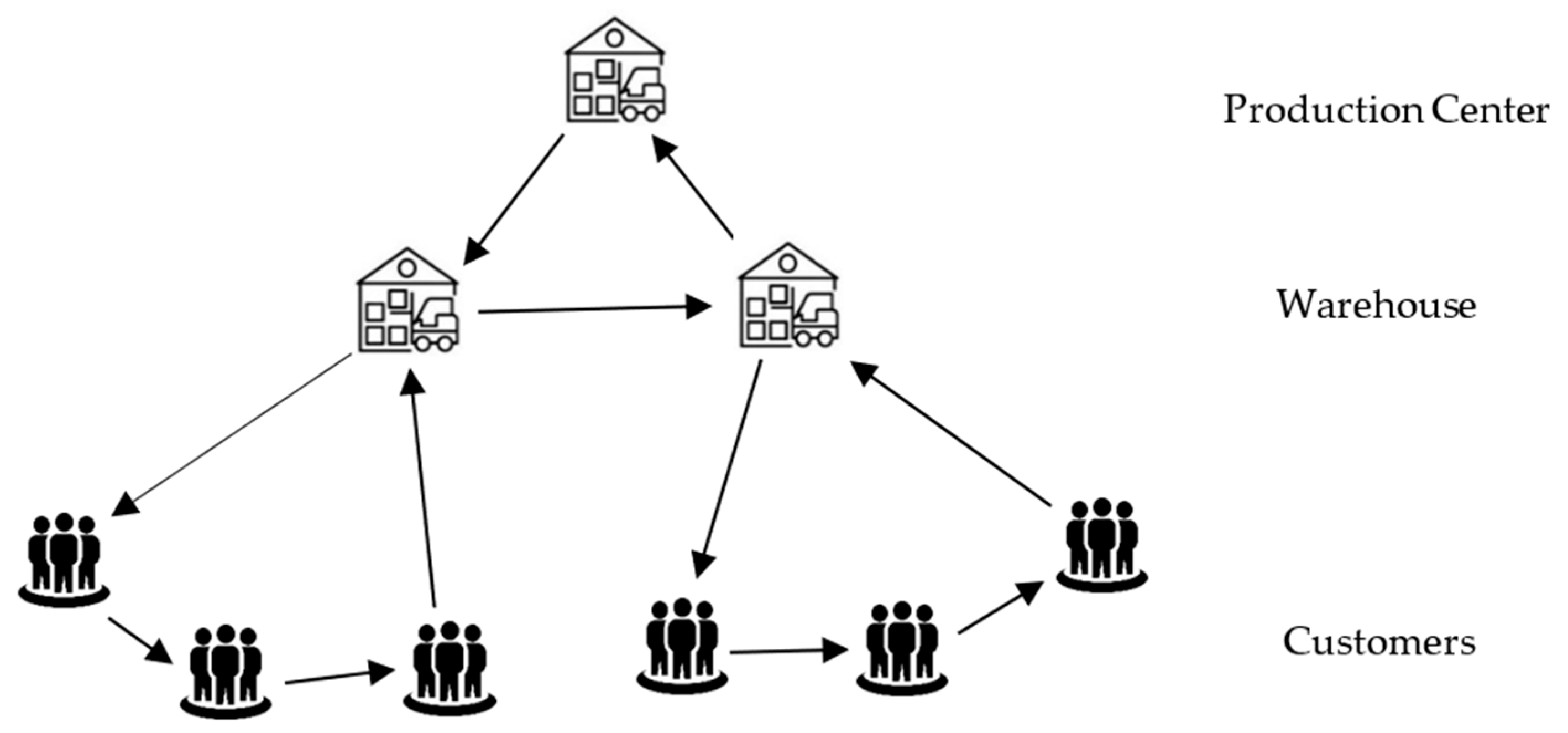
The multi-depot VRP is the general form of VRPs that are used to serve customers. In this problem, each vehicle departs from a depot and returns to the same depot after meeting its customers. This problem has three decision stages. In the first stage, each customer is assigned to a depot and the customers are grouped. Then, in the second stage, a vehicle is assigned to the customers of a group, and finally, in the third stage, the manner and order of meeting the customers is determined by a vehicle. The development of mathematical models for the VRP has led to considering this type of problem at two different echelons, as shown in Figure 1. In this type of problem, which is called an HLRP, the goal of vehicle routing is at the first and second echelons. This type of problem in the first echelon usually uses vehicles with higher capacity, while smaller vehicles are used for vehicle routing from the second echelon. The development of the mathematical model for vehicle routing can lead to a reduction in the total costs of location and routing.

In Figure 1, the network of HLRP including production centers, warehouses, and customers is shown. Adopting strategic decisions, such as determining the location of production centers and warehouses, as well as tactical decisions like vehicle routing between production centers and warehouses and between warehouses and customers, aims to minimize the total costs associated with location and routing. Given the uncertainty in demand and transportation costs, it is recommended to use the fuzzy programming method to manage the model. The model presented in this paper is built on the following assumptions:

• Network levels include production centers, warehouses, and customers.
• All customer demands for different products must be met.
• The amount of demand and transportation costs are uncertain.
• The capacity of production centers and warehouses is known.
• It is a single period and single product model.
• Various types of vehicles are considered.
• The reliability percentage of each vehicle is known.

According to the above assumptions, the optimization model of the FHLRP considering the reliability is presented based on the following symbols. In these symbols, M is a set of potential production centers, $D$ is a set of potential warehouses, $L$ is a set of customers, and $V$ is a set of vehicles ($N_1\in \left\{M\cup D\right\},N_2\in \left\{L\cup D\right\}$).

In this model, the fuzzy programming method is used to deal with uncertainties in the parameters of the created model, i.e., transportation cost and other demand costs. In this method, the linearity of the problem is maintained. In addition, the number of objective functions and constraints remain constant [26]. Due to the computational efficiency and simplicity, the triangular fuzzy distribution method has been used to deal with the inaccurate parameters of the model. Suppose $\tilde{C}$ is a triangular fuzzy number, the membership function of this fuzzy number $\mu \tilde{C}(x)$ is defined as Equation (1):

$$\mu \tilde{C}\left(x\right)=\left\{\begin{array}{cc}{f}_c\left(x\right)=\frac{x-c_p}{c_m-c_p}\hfill & if{c}_p\le x\le c_m\\ 1\hfill & ifx=c_m\\ g_c\left(x\right)=\frac{c_o-x}{c_o-c_m}\hfill & if{c}_m\le x\le c_o\\ 0\hfill & ifx<c_{p}orx>c_o\end{array}\right.$$

(1)

The expected distance $EI$ and the mathematical expectation $EV$ of the triangular fuzzy number are calculated from the following relations:

$$EI\left(\tilde{C}\right)=\left[E_1^c,E_2^c\right]=\left[\underset{0}{\overset{1}{\int }}{f}_c^{-1}\left(x\right)dx,\underset{0}{\overset{1}{\int }}{g}_c^{-1}\left(x\right)dx\right]=\left[\frac{1}{2}\left(c_m+c_p\right),\frac{1}{2}\left(c_o+c_m\right)\right]$$

(2)

$$EV\left(\tilde{C}\right)=\frac{E_1^c+E_2^c}{2}=\frac{c_p+2c_m+c_o}{4}$$

(3)

According to the stated equations, the controlled model of the HLRP is as follows:

$$\begin{array}{ll}MinE\left[OBF\right]=& {\displaystyle \sum _{m\in M}}{fm}_m{Z}_m+{\displaystyle \sum _{d\in D}}{fd}_d{Y}_d+{\displaystyle \sum _{i\in N_2}}{\displaystyle \sum _{j\in N_2}}{\displaystyle \sum _{v\in V}}\left[\frac{c_{vij}^p+2c_{vij}^m+c_{vij}^o}{4}\right]R_{vij}\\ & +{\displaystyle \sum _{i\in N_1}}{\displaystyle \sum _{j\in N_1}}{\displaystyle \sum _{v\in V}}\left[\frac{c_{vij}^p+2c_{vij}^m+c_{vij}^o}{4}\right]X_{vij}+{\displaystyle \sum _{m\in M}}{p}_m{H}_m\\ & +{\displaystyle \sum _{l\in L}}{\displaystyle \sum _{v\in V}}{fv}_v{G}_{vl}+{\displaystyle \sum _{d\in D}}{\displaystyle \sum _{v\in V}}{fv}_v{Q}_{vd}\end{array}$$

(4)

s.t.:

$$\sum _{i\in N_2}\sum _{v\in V}{R}_{vil}\le 1,\hspace{1em}\forall l\in L$$

(5)

$$\sum _{i\in N_2}{R}_{vil}=\sum _{i\in N_2}{R}_{vli}=G_{vl},\hspace{1em}\forall l\in L,v\in V$$

(6)

$$\sum _{d\in D}\sum _{l\in L}{R}_{vdl}\le 1,\hspace{1em}\forall v\in V$$

(7)

$$\sum _{i\in N_2}\sum _{l\in L}\left(\left(1-\alpha \right)\left[\frac{{dem}_l^o+{dem}_l^m}{2}\right]+\alpha \left[\frac{{dem}_l^m+{dem}_l^p}{2}\right]\right)R_{vil}\le c_v,\hspace{1em}\forall v\in V$$

(8)

$$\sum _{i\in L^{\prime }}\sum _{j\in L^{\prime }}{R}_{vij}=\left|L^{\prime }\right|-1,\hspace{1em}\forall v\in V,L^{\prime }\subseteq L,\left|L^{\prime }\right|\ge 2$$

(9)

$$\sum _{d\in D}{B}_{dl}\le 1,\hspace{1em}\forall l\in L$$

(10)

$$\sum _{l\in L}\left(\left(1-\alpha \right)\left[\frac{{dem}_l^o+{dem}_l^m}{2}\right]+\alpha \left[\frac{{dem}_l^m+{dem}_l^p}{2}\right]\right)B_{dl}\le {ca}_d{Y}_d,\hspace{1em}\forall d\in D$$

(11)

$$\sum _{l\in L}{R}_{vdl}+\sum _{i\in N_1}{R}_{vli}-B_{dl}\le 1,\hspace{1em}\forall d\in D,l\in L,v\in V$$

(12)

$$E_{lv}\le c_v\sum _{i\in N_2}{R}_{vil},\hspace{1em}\forall l\in L,v\in V$$

(13)

$$\sum _{l\in L}\sum _{v\in V}{R}_{vdl}=\sum _{i\in N_1}\sum _{v\in V}{X}_{vid}=Y_d,\hspace{1em}\forall d\in D$$

(14)

$$\sum _{d\in D}\sum _{v\in V}{X}_{vmd}\le Z_m,\hspace{1em}\forall m\in M$$

(15)

$$\sum _{j\in N_1}{X}_{vij}=\sum _{j\in N_1}{X}_{vji}=Q_{vi},\hspace{1em}\forall i\in N_1,v\in V$$

(16)

$$\sum _{i\in N_1^{\prime }}\sum _{j\in N_1^{\prime }}{X}_{vij}=\left|N_1^{\prime }\right|-1,\hspace{1em}\forall v\in V,\left|N_1^{\prime }\right|\subseteq N_1,\left|N_1^{\prime }\right|\ge 2$$

(17)

$$\sum _{d\in D}{D}_{dv}\le c_v\sum _{d\in D}\sum _{i\in N_1}{X}_{vij},\hspace{1em}\forall v\in V$$

(18)

$$\sum _{v\in V}{D}_{dv}\le {ca}_d{Y}_d,\hspace{1em}\forall d\in D$$

(19)

$$H_m=\sum _{d\in D}\sum _{v\in V}{D}_{dv}{X}_{vmd},\hspace{1em}\forall m\in M$$

(20)

$$H_m\le {ca}_m{Z}_m,\hspace{1em}\forall m\in M$$

(21)

$$\sum _{i\in N_2}\sum _{j\in N_2}\sum _{v\in V}{e}^{-{\lambda }_v}{R}_{vij}+\sum _{i\in N_1}\sum _{j\in N_1}\sum _{v\in V}{e}^{-{\lambda }_v}{X}_{vij}\ge m\lambda$$

(22)

$$R_{vdl},G_{vl},B_{dl},Y_d,X_{vmd},Z_m,Q_{vd}\in \left\{\mathrm{0,1}\right\}$$

(23)

$$E_{lv},D_{dv},H_m\ge 0$$

(24)

Equation (4) shows the objective function of the mathematical model, which includes minimizing the costs of routing, locating, producing, and deploying multiple vehicles. Equation (5) ensures that each customer is visited only once. Equation (6) guarantees that every vehicle returns to the same warehouse after visiting the customers. Equation (7) indicates that each tour can be completed by at most one vehicle, which means that some vehicles may not be used. Equation (8) states that the amount of product transported by each vehicle does not exceed its capacity. Equation (9) represents the equation related to sub-tour elimination. Equation (10) states that each customer can receive a maximum of one gift from a warehouse. Equation (11) ensures that only the capacity of the selected warehouses can be used. Equation (12) guarantees that if a customer is assigned to a warehouse, one of the vehicles must deliver the product to that customer. Equation (13) shows the maximum quantity of products delivered to each customer. Equation (14) states that if the warehouse is located at node “d”, the vehicle can be moved from that node. Equation (15) shows that if the production center is located at node “m”, the vehicle can pass through that center. Equation (16) states that the vehicle must return to the same center after leaving the production center. Equation (17) represents the equation related to sub-tour elimination. Equation (18) shows the amount of product distributed by each production center, and Equation (19) ensures that this volume of distribution does not exceed the capacity of the center. Equations (20) and (21) also represent the equations related to the volume of products produced by each located production center. Equation (22) guarantees the establishment of the minimum reliability of the entire network by considering the different capabilities of the vehicles in the network. Equations (23) and (24) also represent the type of decision-making variables.

In this section of the paper, the modeling of the FHLRP is discussed. Considering that the problem under investigation is NP-hard, GA, and PSO have been used to solve it. The subsequent section covers the initial solution and parameter tuning of GA and PSO using the Taguchi method.

4. Solution Methods

4.1. Designing the Initial Solution

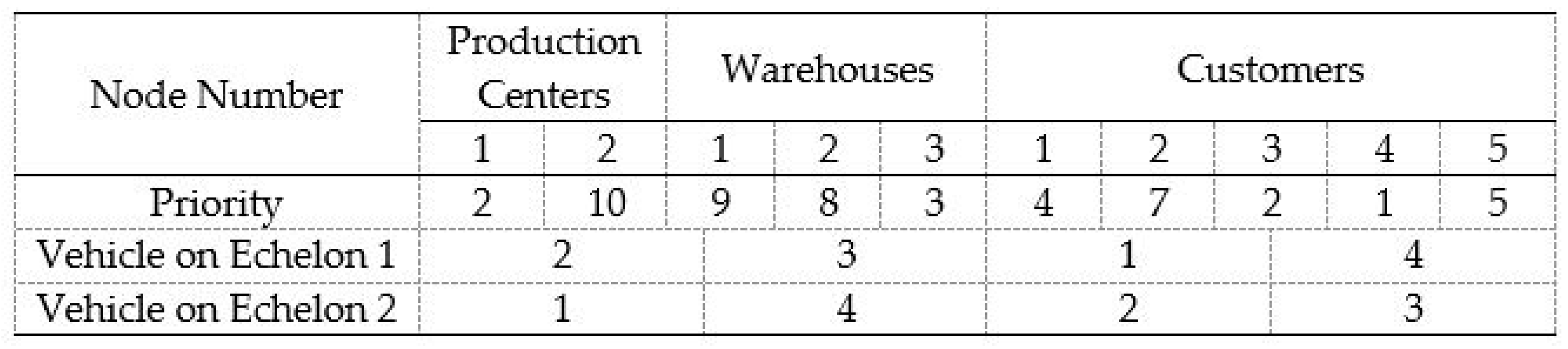
The most important issue in solving mathematical models with GA and PSO is designing the initial solution. This solution should be designed in such a way that it can lead to the exploration of the entire problem space by the algorithms used. In Figure 2, we consider the initial solution for a hypothetical example that includes 2 production centers, 3 warehouses, 5 customers, and 4 types of vehicles.

To decode the solution presented in Figure 2, the following steps are performed in order:

• Part 1: Location

Step 1: Calculate total customer demand.

Step 2: Choose the highest priority among the warehouses and compare the capacity of that center with the total demand (the highest priority among the warehouses is warehouse number 1 with priority 9).

Step 3: If the capacity of this warehouse alone does not meet the demand, choose the warehouse with the next highest priority.

Step 4: Continue step 3 until the warehouse capacity meets the total demand and reduce the priority of unselected warehouses to 0.

Step 5: Select the highest priority among the production centers and compare the capacity of that center with the total demand (the highest priority among the production centers is production center number 2 with priority 10).

Step 6: If the capacity of this center alone does not meet the demand, select the production center with the next highest priority.

Step 7: Continue step 6 until the capacity of production centers meets the total demand and reduce the priority of unselected production centers to 0.

Step 8: Warehouses and production centers whose priority is not 0 are selected as actual warehouses and production centers.

• Part 2: Vehicle routing between warehouse and customers

Step 1: Select the first vehicle from the vehicle preferences in echelon 1 (Vehicle 2 will be selected).

Step 2: Select the highest priority among clients as the first visiting node (client 2 with priority 7 is selected).

Step 3: The sequence of customer visits by the selected vehicle continues until the vehicle capacity is less than the customer demand.

Step 4: If all customers have not been visited, the next vehicle is selected and steps 1 to 3 are repeated.

• Part 3: Vehicle routing between production centers and warehouses

Step 1: Select the first vehicle from the vehicle preferences in echelon 2 (Vehicle 1 will be selected).

Step 2: Select the highest priority among warehouses with no priority 0 as the first visited node (warehouse 1 is selected with priority 9).

Step 3: The sequence of visits to the warehouses by the selected vehicle continues until the vehicle capacity is less than the demand of the warehouses.

Step 4: If all non-priority warehouses have not been visited, the next vehicle is selected and steps 1 to 3 are repeated.

• Part 4: Calculation of the objective function

After determining the main decision variables of the problem, the total cost of the network is calculated.

4.2. Parameter Tuning

At this stage, before solving the large-scale problem using solution methods, GA and PSO parameters are adjusted by the Taguchi method. In the Taguchi method, the appropriate factors must be identified first. Then, the levels of each selection factor and the appropriate test plan for these control factors should be determined. After determining the test plan, the tests are performed and analyzed with the aim of finding the best combination of parameters. In this paper, based on

Table 1. Parameter tuning of GA and PSO by Taguchi method.

Solution Method	Factor	L1	L2	L3	Optimum Value
GA	Max it	100	150	200	200
	N pop	100	150	200	200
	Pc	0.7	0.8	0.9	0.7
	Pm	0.05	0.06	0.07	0.06
PSO	Max it	100	150	200	200
	N particle	100	150	200	200
	C1	1	1.5	2	1.5
	C2	1	1.5	2	2
	w	0.5	0.6	0.8	0.5

, three levels are considered for each factor. The design of the test and its implementation are determined for each algorithm, considering the number of factors and the number of their levels.

According to the minimization of the total costs in the proposed model, the amount of each test should be calculated first. After determining the value of each test, the unscaled value of each test (RPD) is calculated from $\frac{S_i-S_i^{\mathrm{*}}}{S_i^{\mathrm{*}}}$ to analyze the Taguchi test design. In the above relationship, $S_i$ is the value obtained from each Taguchi test and $S_i^{\mathrm{*}}$ is the best value of all tests.

4.3. TOPSIS Method

TOPSIS, as one of the MCDM methods, considers both the distance of each alternative from the positive ideal and the distance of each alternative from the negative ideal point. In other words, the best alternative should have the shortest distance from the positive ideal solution (PIS) and the longest distance from the negative ideal solution. The steps of the TOPSIS method are described below:

• Step 1: Normalize the decision matrix

The following formula can be used to normalize.

$$r_{ij}\left(x\right)=\frac{x_{ij}}{\sqrt{{\sum }_{i=1}^m{x}_{ij}^2}},\hspace{1em}\forall i,j$$

(25)

• Step 2: Calculate the weighted normalized decision matrix

According to the following formula, the normalized matrix is multiplied by the weight of the criteria.

$$v_{ij}\left(x\right)=w_j{r}_{ij}\left(x\right),\hspace{1em}\forall i,j$$

(26)

• Step 3: Determine the positive ideal and negative ideal solutions

The aim of the TOPSIS method is to calculate the degree of distance of each alternative from positive and negative ideals. Therefore, in this step, the positive and negative ideal solutions are determined according to the following formulas.

$$A^{+}=\left(v_1^{+},v_2^{+},\dots ,v_n^{+}\right);A^{-}=\left(v_1^{-},v_2^{-},\dots ,v_n^{-}\right)$$

(27)

So that

$$v_j^{+}=\left\{\left(max{v}_{ij}\left(x\right)|j\in j_1\right),\left(min{v}_{ij}\left(x\right)|j\in j_2\right)\right\};v_j^{-}=\left\{\left(min{v}_{ij}\left(x\right)|j\in j_1\right),\left(max{v}_{ij}\left(x\right)|j\in j_2\right)\right\}$$

(28)

where $j_1$ and $j_2$ denote the negative and positive criteria, respectively.

• Step 4: Distance from the positive and negative ideal solutions

TOPSIS method ranks each alternative based on the relative closeness degree to the positive ideal and distance from the negative ideal. Therefore, in this step, the calculation of the distances between each alternative and the positive and negative ideal solutions is obtained by using the following formulas.

$$d_j^{+}=\sqrt{\sum _{j=1}^n{\left[v_{ij}\left(x\right)-v_j^{+}\left(x\right)\right]}^2},\hspace{1em}\forall i;d_j^{-}=\sqrt{\sum _{j=1}^n{\left[v_{ij}\left(x\right)-v_j^{-}\left(x\right)\right]}^2},\hspace{1em}\forall i$$

(29)

• Step 5: Calculate the relative closeness degree of alternatives to the ideal solution

In this step, the relative closeness degree of each alternative to the ideal solution is obtained by the following formula. If the relative closeness degree has value near to 1, it means that the alternative has shorter distance from the positive ideal solution and longer distance from the negative ideal solution.

$$C_i=\frac{d_j^{-}}{\left(d_j^{+}+d_j^{-}\right)}\forall i$$

(30)

5. Analysis of the Results

5.1. Validation of the Model

In this section, a numerical example is considered to validate the presented mathematical model. The example includes three production centers, four warehouses, six customers, and eight vehicles. Random data has been used due to the lack of access to real-world data. The data are generated based on the uniform distribution function as described in

Table 2. Interval boundaries of deterministic and uncertainty parameters.

Parameter	Value	Parameter	Value
${dem}_l^o$	$~U\left(100,150\right)$	$c_{vij}^o$	$~U\left(30,40\right)$
${dem}_l^m$	$~U\left(150,200\right)$	$c_{vij}^m$	$~U\left(40,50\right)$
${dem}_l^p$	$~U\left(200,250\right)$	$c_{vij}^p$	$~U\left(50,60\right)$
$c_v$	$~U\left(400,500\right)$	$p_m$	$~U\left(2,5\right)$
${ca}_d$	$~U\left(600,800\right)$	${fv}_v$	$~U\left(1000,1500\right)$
${ca}_m$	$~U\left(700,1000\right)$	${fd}_d$	$~U\left(\mathrm{10,000},\mathrm{12,000}\right)$
${fm}_m$	$~U\left(\mathrm{10,000},\mathrm{12,000}\right)$

. These values are sourced from articles related to the topic and are used to justify the solution space.

In the presented numerical example, the results of the first part are presented assuming an α = 0.5, due to the use of the fuzzy programming method in controlling uncertainty parameters. An uncertainty rate of 0.5 represents the encounter of the middle state in the optimization model. The optimal value of the objective function of the stated numerical example is USD 45,823.83 at 97.45 s. These results are the outcome of implementing the model in GAMS 24.8.2 software and using the Baron Solver. The outputs from the numerical example are shown below. Figure 3 displays the location of production centers and warehouses, along with the routing of vehicles on the first and second echelon.

According to Figure 3, it can be seen that production center number (1) was selected from three potential centers, and two warehouses number (2) and (4) were located from four potential warehouses. The total cost obtained from the numerical example in a small size consists of location costs (USD 33,968.04), vehicle deployment cost (USD 10,755.77), transportation cost (USD 550.40), and production cost (USD 3249.62). These reasons show that the biggest costs incurred in the network are location costs or making strategic decisions.

In the following, the cost changes of the whole model presented in different scenarios have been investigated.

Table 3. Total cost changes in different scenarios.

$\mathit{\alpha }$	Total Cost (USD)	Changes (%)
0.1	39,527.61	−13.74
0.2	41,688.30	−9.02
0.3	43,685.58	−4.67
0.4	44,124.15	−3.71
0.5	45,823.83	0
0.6	46,937.18	+2.43
0.7	48,536.33	+5.92
0.8	52,348.66	+14.26
0.9	54,366.47	+18.64
${\mathit{c}}_{\mathit{v}}\left(\mathbf{\%}\right)$	Total Cost (USD)	Vehicle Number
−30	46,238.44	5
−20	46,238.44	5
−10	45,823.83	4
0	45,823.83	4
+10	45,823.83	4
+20	44,259.67	3
+30	43,211.28	3
${\mathit{c}\mathit{a}}_{\mathit{d}}-{\mathit{c}\mathit{a}}_{\mathit{m}}\left(\mathbf{\%}\right)$	Total Cost (USD)	Total Centers
−30	58,947.22	4
−20	58,647.66	4
−10	45,823.83	3
0	45,823.83	3
+20	45,823.83	3
+30	31,246.91	2

shows the changes in the total cost of the problem at different uncertainty rates, vehicle capacity, and production center capacity.

The results from Table 3 indicate that total costs have increased as the uncertainty rate has increased. This increase in costs is attributed to the rise in customer demand. As the demand has increased, along with the stability of other factors, the number of vehicles needed has also increased, resulting in higher overall costs. Additionally, the reduction in vehicle capacity has necessitated the use of more vehicles, further driving up costs for vehicle usage and routing. Consequently, reducing the vehicle capacity by 30% has led to a change in the number of vehicles required, increasing from four to five.

On the other hand, changes in facility capacity also affect total costs. As facility capacity decreases due to a decrease in supply, a larger number of facilities are required to meet all customer demand. This issue results in an increase in the fixed costs of locating the facility, thereby increasing the total costs.

5.2. Analyzing a Small Numerical Example with GA and PSO

In this section, before solving various numerical examples, we have conducted an analysis of a small-sized numerical example using GA and PSO and compared the results with those obtained from Baron. Consequently, by keeping the size and value of the mathematical model’s parameters constant, we present the convergence of the solution methods over 200 consecutive iterations in Figure 4.

After solving the problem using GA and PSO, the total cost obtained by GA is USD 46,093.17 and by PSO is USD 46,187.18. Therefore, the maximum percentage of the relative difference between the solutions of the algorithms and the optimal solution is 0.587% and 0.792%, respectively. Additionally, the problem-solving time for GA was 15.67 s and for PSO was 12.55 s.

Table 4. Location and routing obtained from the solution of a small numerical example.

Solution Methods	Production Centers	Warehouse	Customer	Optimum Routing	Vehicle Number
Baron	1	2-4	-	$M_1\to D_2\to D_4\to M_1$	2
	-	2	1-5	$D_2\to L_5\to L_1\to D_2$	3
	-	2	2	$D_2\to L_2\to D_2$	1
	-	4	3-4-6	$D_4\to L_4\to L_6\to L_3\to D_4$	4
GA	1	2-4	-	$M_1\to D_2\to D_4\to M_1$	3
	-	2	1-2	$D_2\to L_2\to L_1\to D_2$	2
	-	2	3	$D_2\to L_3\to D_2$	1
	-	4	4-5-6	$D_4\to L_4\to L_6\to L_5\to D_4$	4
PSO	2	1-4	-	$M_1\to D_1\to D_4\to M_1$	1
	-	1	4-6	$D_1\to L_4\to L_6\to D_1$	4
	-	1	3	$D_1\to L_3\to D_1$	2
	-	4	1-2-3	$D_4\to L_2\to L_1\to L_3\to D_4$	3

displays the location and routing obtained from solving a small numerical example using different solution methods.

5.3. Analysis of Large Numerical Examples with GA and PSO

After examining the decision variables of the numerical example of small size using different solution methods, it was observed that the maximum percentage of relative difference between the solution methods and Baron is less than 1%. Therefore, numerical examples of different sizes were analyzed.

Table 5. Size of numerical examples in different scales.

Sample Problem	Production Center	Warehouse	Customers	Vehicles
1	5	6	7	6
2	5	6	8	8
3	8	6	10	10
4	8	8	12	12
5	10	8	15	14
6	10	8	18	16
7	12	10	20	18
8	12	10	23	20
9	15	10	28	22
10	15	12	32	24
11	18	12	35	26
12	18	15	40	28
13	20	15	45	30
14	25	18	50	32
15	30	20	60	35

presents the 15 numerical examples in different sizes in ascending order.

After designing various numerical examples, the best solution obtained from running GA and PSO three times is presented in

Table 6. Total costs and solution time obtained from solving different numerical examples.

Sample Problem	Total Cost (USD)			CPU-Time (s)
	Baron	GA	PSO	GAMS	GA	PSO
1	69,745.28	70,391.12	70,370.21	128.49	21.72	18.66
2	88,672.24	89,589.11	89,730.15	331.97	23.63	20.37
3	95,748.66	96,822.96	96,837.32	597.29	27.77	23.94
4	112,343.28	114,075.63	113,857.73	972.66	32.91	28.37
5	-	127,890.05	125,566.02	<1000	40.32	34.76
6	-	141,782.57	142,023.64	<1000	52.40	45.17
7	-	161,659.52	162,441.07	<1000	69.59	59.99
8	-	172,868.33	176,139.36	<1000	89.09	76.80
9	-	192,507.95	194,335.84	<1000	111.87	96.44
10	-	209,109.05	208,593.57	<1000	144.69	124.73
11	-	221,201.84	222,350.19	<1000	193.12	166.48
12	-	235,330.92	235,916.97	<1000	249.01	214.66
13	-	257,636.53	260,863.93	<1000	313.00	269.83
14	-	283,291.13	285,776.63	<1000	400.05	344.87
15	-	298,740.32	299,020.68	<1000	488.21	429.47

. Additionally, this table also includes the time taken to solve different numerical examples using different solution methods.

The results of Table 6 show that Baron was unable to solve numerical examples greater than five, resulting in a solving time of more than 1000 s. Additionally, the results demonstrate that PSO has been more successful in solving various numerical examples in a shorter amount of time compared to GA. On average, GA has exhibited greater efficiency than PSO in the search for a near-optimal solution. 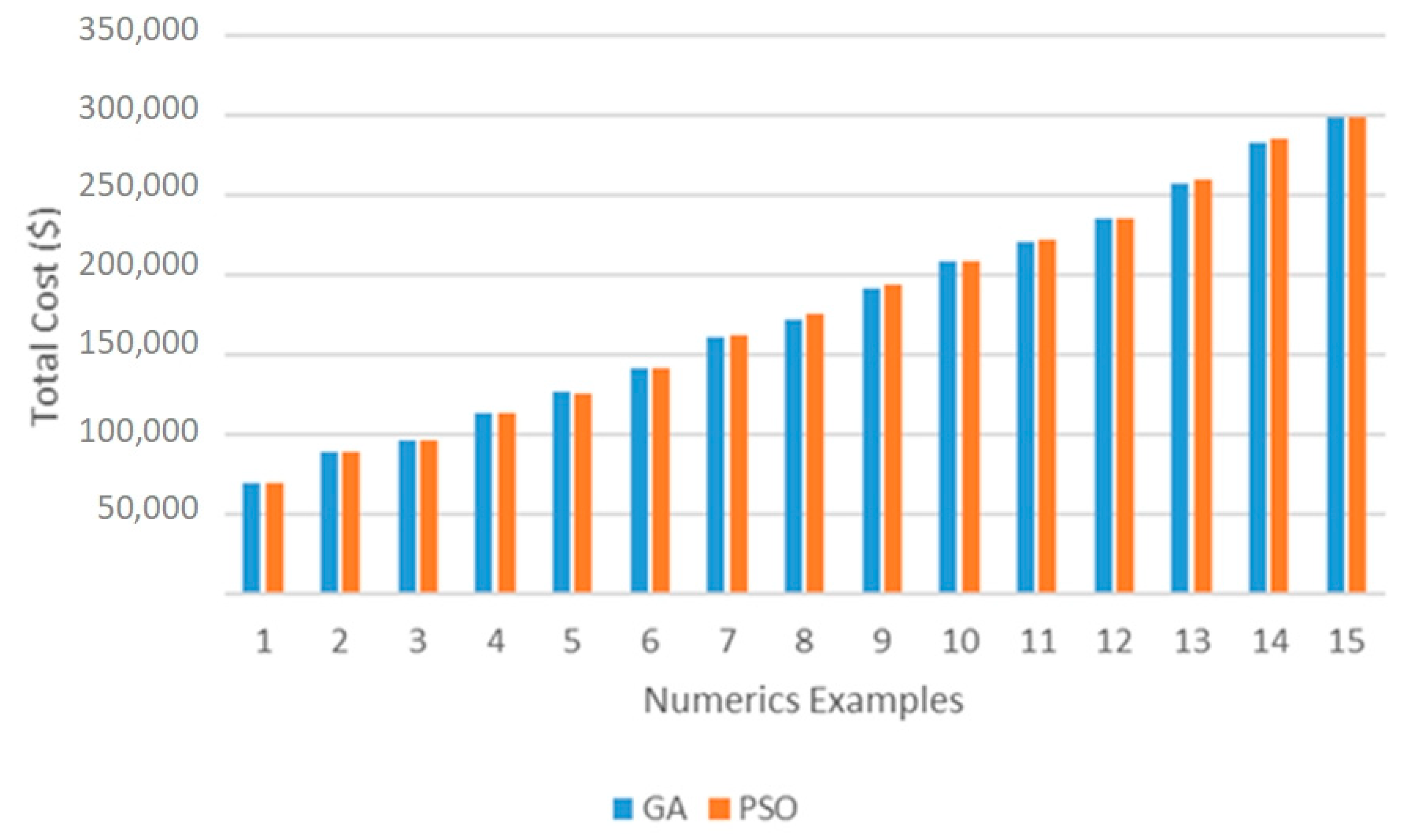Figure 5 and Figure 6 display the best objective function and computational time achieved by different solution methods when dealing with large-sized numerical examples.

The analysis of numerical examples in different sizes showed that GA was more efficient than PSO in obtaining near-optimal solutions. However, PSO achieved the final results in less time. Therefore, since there is no ranking of different solution methods, the TOPSIS method has been used. In this paper, there are two criteria (mean of objective function and mean of CPU-Time) and two alternatives (GA and PSO) that are ranked using the TOPSIS method.

Table 7. Characteristics of criteria, decision, and normalized matrix.

Solution Method	Mean of Objective Function	Mean of CPU-Time
GA	178,193.1	150.49
PSO	178,921.6	130.30
Weight	0.5	0.5
Type	Negative	Negative
Normalized
GA	0.706	0.756
PSO	0.709	0.655

shows the main characteristics of criteria and decisions and the normal matrix.

Table 8. The positive and negative ideal values.

Solution Method	Mean of Objective Function	Mean of CPU-Time
GA	0.353	0.354
PSO	0.327	0.378
	Distance to positive ideal	Distance to positive negative
GA	0.051	0.001
PSO	0.001	0.051

shows both positive and negative ideal values and the distance to the positive and negative ideal solutions.

The results, considering the preference weight of 0.5 for each criterion, show that GA was more efficient than PSO with a preference weight of 0.972.

6. Conclusions

In this paper, a FHLRP model is presented with the main goal of minimizing the costs associated with locating potential warehouses, production centers, and vehicle routing. To address uncertainty, a nonlinear mathematical model is designed and a fuzzy programming method is used to control the uncertainty parameters. The validation results of the mathematical model demonstrate that as the uncertainty rate increases, the total costs also increase, primarily due to an increase in customer demand. Additionally, the results show that a decrease in vehicle capacity leads to a higher number of vehicles needed, resulting in increased costs for vehicle usage and routing. For instance, a 30% reduction in vehicle capacity results in a change from four to five vehicles. Furthermore, the changes in facility capacity have a significant impact on the overall costs of the model. A decrease in facility capacity leads to a higher number of facilities required to fulfill customer demand due to a decrease in supply. Considering the NP-hard nature of the mathematical model, both GA and PSO are employed to solve the problem. The analysis of the numerical example exhibits that the maximum relative difference percentage between the algorithm solutions and the optimal solution is 0.587 and 0.792, respectively. Moreover, GA has a problem-solving time of 15.67 s, while PSO takes 12.55 s. Based on these findings, both algorithms are utilized to solve numerical examples of larger sizes. Further analysis of 15 numerical examples demonstrates the inefficiency of Baron in solving larger numerical examples. In terms of near-optimal solutions, GA proves to be more efficient compared to PSO, though PSO achieves results in less time. Therefore, the TOPSIS method is employed to rank the different solution methods. The results, with a preference weight of 0.5 assigned to each criterion, indicate that GA is more efficient than PSO with a preference weight of 0.972.

One of the limitations in dealing with the problem is the lack of access to real-world data, as well as historical data. Another limitation is the implementation of the mathematical model in the real world, which is hindered by the lack of financial information provided by organizations.

As future suggestions, it is important to consider social aspects in the developed mathematical model. Additionally, the fuzzy robust method should be employed to control the uncertainty parameters of the problem. Opening the Jackson network for distributing items to customers is also recommended. Finally, using hybrid algorithms to solve the problem is suggested.