A New Model for Determining the Price of Product Distribution Based on Fuzzy Logic

Abstract

Background: Distribution is a very important part of logistics and an activity that is present in every area today. One of the basic problems in distribution is how to correctly determine its price. For this reason, this paper presents a model created to determine the price of the product distribution service. Methods: The model first determines the base of the distribution price, which consists of a fixed and a variable part. The fixed part depends on the distance traveled, and the variable part is defined by fuzzy logic. To determine the variable part, a fuzzy logic system was created that depends on four input variables: inaccessibility of the client’s location, driving time, quantity of goods, and unloading time. The reason for applying fuzzy logic is its ability to set the distribution price for each client individually, without generalization. Certain criteria that affect the distribution price such as type of vehicle, quality of service, and type of goods, which could not be represented by fuzzy numbers, were considered as additional corrective factors. Results: The model was tested on hypothetical examples created by the authors from this field and on examples of company that provide distribution services. In the case study, a comparison was made between the distribution price obtained by applying the created fuzzy logic model and the price defined by the model used by the company "X". Conclusions: The model created in this way enables easy adaptation to constant changes in the prices of oil derivatives due to the COVID-19 pandemic and the war but also considers various unpredictable circumstances that may occur during delivery such as roadworks, crowds, vehicle breakdown, location inaccessibility due to bad weather, etc.

1. Introduction

The daily needs of people have led to distribution becoming one of the most represented activities. Whether they need food and necessities, furniture for the house, or home delivery, distribution is necessary. A difference should be made between the distribution of services and the distribution of material products. Namely, the distribution of services is specific and significantly different from the placement of material products, which results from the specific features of the service product. Some of the basic questions posed to a service system include through which distribution channels the service will be delivered, at what time the service will be performed, and where (at which location) the service will be provided. However, the focus of this paper is the distribution of material products and the determination of the price that needs to be paid in the case of the delivery of certain goods from point A to point B. It could be said that the distribution of services is not entirely possible without the distribution of material products.

The price of the distribution service in logistics is very important because it should simultaneously cover all generated costs and make a profit. On the other hand, it must not be too high, because it will reject the client. Strict market requirements, strong competition, and increasingly demanding customers set additional requirements in terms of reducing total costs and increasing business efficiency. To correctly define the price of the distribution service, it is necessary to identify all costs. Logistics costs account for between 25% and 45% of total costs and up to 20% of product prices, depending on the activity and type of business [1]. In logistics, the most important costs are transport and storage costs [2]. Depending on the size of the company, the type of business, the development of the economy, and many other factors, transport costs have the largest share in the total costs of logistics (from 25% to 50%) [1]. The correct determination of the price of the distribution service plays the main role in covering transport costs. However, due to major changes and instability in the market in the last two or three years, the price of distribution is increasingly difficult to define. Unpredictable situations during the distribution of products lead to the fact that the price charged for the provided service in certain situations cannot even cover the costs themselves. For this reason, the goal of this paper was to develop a model for determining the price of distribution services that will be easily adaptable to the increasingly frequent changes in the market in terms of energy prices and the unpredictable circumstances due to the emergence of the COVID-19 pandemic, and which will enable the company to have a more accurate and realistic price that will set it apart from the competition. The available models in the literature for determining the price of the distribution service, such as the models developed in the papers [3,4] are not able to properly respond to the new changes in the market. The models in the papers [3,4] define the cost of distribution in advance before the service is realized so if during the realization of the service the delivery of goods takes a longer time due to congestion or roadworks, those costs will not be included in the price and this will represent a cost for the company. Also, due to the protest and the closure of certain parts of the city, the vehicle may take a different route instead of the planned one, so the distribution costs will be higher, but they will not be taken into account when forming the price because it is defined in advance. The model created in this paper enables all costs to be covered, regardless of irregularities during the realization of goods delivery, and ensures that clients are satisfied with the price. In addition, its objectivity sets the company apart from the competition. Also, it should be emphasized that the model is simple to use and can be very easily applied in practice. It should be noted that no matter how good the pricing model is, it can be even better if the business efficiency of the distribution company is increased. Efficiency can be increased by better utilization of resources, but also by reducing costs, which can be measured and analyzed using the DEA method [5,6,7]. By using the DEA method for decision support, there is an opportunity for the correction of the price of the distribution service, in terms of providing a cheaper service compared to the competition.

In the next chapter of the paper, there is a detailed description of the solved problem and a literature overview. The fourth chapter describes in detail the model developed in this paper, which is used to determine the price of the product distribution service. After that, the model was first tested on hypothetical examples in chapter five, after which a sensitivity analysis of the created model was performed. In chapter six, the model is tested on the example of a company “X”, which provides a distribution service, and has its model for determining the distribution price. Also, in chapter six, managerial implications are given based on model testing. Concluding considerations and future research directions are given at the end of the paper.

2. Problem Description and Literature Review

This chapter aims to identify problems that arise when determining the price of distribution, as well as potential solutions to those problems. Also, in the rest of the chapter, a brief literature analysis on the topic of pricing in distribution will be given.

2.1. Problem Points, Motivation, Potential Solutions, and Novelties

One of the basic problems that arises regarding distribution is how to determine the distribution price properly. It is very difficult to “estimate” the distribution so that all clients are equal and the service provider is satisfied with the profit. In practice, there are numerous ways to determine the price of distribution, from self-assessment in some small companies to very complex models in large companies. The evaluation criteria are numerous, and the priorities differ from distributor to distributor. For some providers, the most important thing will be fuel consumption, while for others, the quality of the service will be more important, to keep their clients. Regardless of the importance of the criteria, some that almost always appear and are key to determining the distribution price are the distance (traveled kilometers), driving time, quantity of transported goods, quality of service, location of the client, and others.

However, the main problem, whether using an independent assessment or a developed model, is the impossibility of accurately and precisely determining the price for each client. For this reason, there is inequality in the treatment of each client, and potentially dissatisfaction or, in the end, termination of use of the distribution service. All this happens due to the generalization of similar situations and not using stochastics. Most distributors use the so-called tabular approach. If, for example, the criterion is kilometers driven, distributors will use a table with certain ranges or classes and their corresponding prices per kilometer [8]. The problem in this case arises if, for example, the distance to client 1 is equal to the left limit of the range, and the distance to client 2 is equal to the right limit of the range. This would mean that according to the distance criterion, these clients will be charged the same price per kilometer, which is not equal for client 1, for whom the distance is shorter in comparison to client 2. A similar problem would occur if the quantity or driving time were taken as a criterion.

The wrong price of the distribution service can also be obtained in case of neglect or exclusion of important criteria. For example, many developed models in practice do not consider the quality of the service, which is a big omission. In this way, damage to the goods during transport or delivery, which happens very often, is not taken into account. In the same way, neglecting quality also means a delay in delivery or delivery of the wrong goods (or quantity). All this should be an integral part of the price through benefits in the case of high-quality service or a certain penalty in the case of poor quality. Also, distributors rarely take into account the location where the client is located, which again causes the wrong price because the location significantly affects fuel consumption. Namely, if there is a client located in a suburban location that requires driving on “open” roads, his price cannot be the same as for a client located in a mountainous area that is reached by rural roads. A big problem when determining the price of distribution is that the price is formed in advance, before the actual realization of the process. In this way, unforeseeable circumstances that may occur during the implementation of the distribution, such as congestion in the city, roadworks, vehicle breakdown, etc., cannot be taken into account in the distribution price. All these unpredictable circumstances can lead to an increase in distribution costs, and therefore the distribution price should be higher. Also, in a situation where the distribution is realized before the scheduled time without interfering factors, the price of the distribution should be lower than the one previously agreed.

It can be concluded that problems in determining the distribution price are the use of deterministic only but also the exclusion of some important criteria. To potentially overcome these problems, it is suggested to apply a fuzzy logic that will take into account stochasticity, as well as an attempt to consider all the key criteria that affect the price. Also, based on what has been described, it can be concluded that one of the important problems when generating the distribution price is the existence of two conflicting parties, clients on the one hand and service providers on the other. For both parties to be satisfied, it is necessary to devise a model that will create a balance between them and define the price in following the real conditions that occurred during the realization of the distribution. However, no interested party would agree to complete uncertainty when defining the distribution price if it were to be defined after the realized service, and not before. Therefore, in this paper, a model was created that consists of two parts, fixed and variable. A fixed part of the price of the distribution is formed before the actual realization of the service so that the users of the service can know the approximate price of the distribution in advance and do not have complete uncertainty about the price. The variable part is formed after the service has been provided and it varies depending on the conditions that occur during the realization of the service. It is this variable part that ensures the balance between two interested parties, who have conflicting interests. By applying the model created in this paper, the generalization of the distribution price for users is overcome. Instead, the service price is generated for each user following the circumstances under which it is realized. In this way, users can sometimes pay less and sometimes more for the same service if that service is provided under different circumstances. The model created in this paper assures service providers that their costs will always be covered. The model also enables lower distribution prices for the user, because when generating the price, service providers do not have to take into account the costs of unforeseen circumstances that may occur during the realization of the service.

In the literature search, no approach was found that defines the cost of distribution in two parts, before and after the realized service. All approaches in the searched literature determine the cost of distribution in advance before the service is realized. The advantage of this approach is that it provides benefits for both service providers and service users. Also, most of the approaches in the literature cannot be applied without major changes in different companies, in different countries, while the approach developed in this paper can be easily applied in practice by modifying the distribution price per kilometer driven. It should be noted that the model developed in this paper is very resistant to various changes in the market due to disruptions such as pandemics, war, crises, etc.

2.2. Literature Review

Although the problem of distribution and determining the price of this service is a very common topic in the field of logistics, most of the papers in the literature refer to the determination of total logistics costs. Logistics costs make up a significant and largest part of business costs, which often exceed 10% of the company’s turnover [9]. For this reason, most scientific papers deal with the analysis of logistics costs in general, the development of models for their calculation, and potential options for their optimization. For example, the paper on “Multiple-method analysis of logistics costs” [9] examines the differences and interdependencies in the logistics costs of trading companies operating in Finland. The authors indicate that total logistics costs consist of six individual components: transportation, warehousing, inventory holding, administrative costs, and transport packaging (loading and unloading). Logistics costs have been investigated through multiple methods, including descriptive analysis, generalized linear mixed models (GLMM), and principal component analysis [9]. Time, number of employees, turnover, industry, and level of internationalization were shown as statistically significant variables of logistics costs. In general, the analysis indicates the need for caution in interpreting changes in logistics costs and simultaneously controlling for the effects of background variables.

Accurately calculating logistics costs has become a real challenge in logistics and supply chain management. It is essential to obtain reliable and accurate cost information to achieve an efficient allocation of resources within logistics service companies. Traditional costing approaches may sometimes not be sufficient to achieve this goal in the case of complex and heterogeneous logistics service structures. Therefore, many authors tend to explore ways to improve the cost calculation methods of logistics service providers. For example, the author Bokor in the paper “Cost Calculation Model for Logistics Service Providers” tries to show how it is necessary to adopt the so-called multi-level technique of allocating costs in logistics practice [10]. After determining the methodological framework, the author develops a calculation scheme and tests it using estimated input data. Based on the theoretical findings and experiences of the pilot project, it is concluded that the improved cost accounting model contributes to making logistics costs more precise and transparent. Moreover, the relationships between costs and performance also become more visible, which significantly increases the efficiency of logistics planning and control.

However, there are also papers in the literature that specifically deal with the distribution service and the costs it causes. One such paper is “Developing a Distribution Pricing Model for the Case Company” by Ketola [3]. This is a case study that was applied to the example of the leading Finnish brewery “Sinebrychoff”. The author first analyzes the current situation in the company, where he first gets acquainted with the current model that the company uses to calculate the distribution price [3]. After the analysis, the author researches the best methods from practice to create a framework for a new price calculation model. Finally, the company is proposed to use a new distribution price model with an explanation of its constituent elements and how to apply it. This study is based on real data obtained through measurement and interview techniques. The interview technique was applied to the employees of the Sinebrychoff company to obtain the real data needed for the analysis.

The problem of determining the price of the distribution service was addressed in the paper “Pricing Strategies of Logistics Distribution Services for Perishable Commodities” [4]. In their study, four logistics service pricing strategies were constructed, including a fixed pricing model, a fixed pricing model with time constraints, a dynamic pricing model, and a dynamic pricing model with time constraints. Each of these strategies is combined with factors such as delivery time, customer satisfaction, etc. Analysis of the average profit of logistics service providers in these four pricing models shows that the average profit in the dynamic pricing model with time constraints is the highest.

In an article published in 2020 by the author Walts, several factors affect the price of a distribution service, and a few ways to determine the price are presented [11]. A “good” price for the distribution service is essential, as it allows the company to stand out from many competitors. Author Walts notes that to be able to determine the right price, it is first necessary to identify all the costs that arise during the realization of the service, such as the cost of boxes, packages, tapes and stickers, labor costs, transport costs, etc. If the price is too low, the company will operate in the red, and if the price is too high, the company will lose business due to competition. For this reason, the application of the right pricing model is of great importance. One way of calculating the price is to form it based on the weight and volume of the goods and the distance traveled. However, the problem arises in the case of irregularly shaped goods and many smaller shipments. Another way to calculate the price is a flat rate for each service performed. Regardless of the quantity of goods, the distance of the client, etc., the same amount is always paid. This model is suitable for use by smaller companies, whose service area is small and homogeneous. The third, widely used way is to provide the distribution service completely free of charge. In that situation, the company has two ways to cover its costs. First, to incorporate delivery costs into their products, thereby increasing the price of the product compared to the competition. Another option is to minimize costs by using collective deliveries and reducing the margin with the expectation of increasing sales. Also, this model is suitable for retail companies. The author of the article singles out four basic elements for calculating the price of the distribution service: distance, volume, mass, and expected delivery time. The remaining factors that can affect the price depend on the type of goods, the specifics of the requirements, and the need for additional workers.

In the paper [12], the authors propose a ranking method when choosing a distribution service provider. In their paper, they emphasize numerous criteria based on which the user chooses a distribution service provider. One of the most important criteria that influence the choice of a company that implements the distribution service is the distribution price. Therefore, the company needs to use a model for determining the distribution price that provides benefits to users through a lower price of the service, higher quality, charging a lower price due to lower costs during the implementation of the service, etc.

The authors of the paper [13] note that for proper cost management in transport logistics, it is necessary to optimize all stages of the transport–logistics process, from the selection of the type of transport and the construction of the supply chain to the planning of routes and the monitoring of the execution of tasks. In the paper, the authors deal with determining the price of goods transportation, considering internal and external influencing factors. The results of the research show that the transport company should have different payment options for the service performed, depending on the type of vehicle with which the service was performed, then they should provide three types of transportation prices: price/m³, t, km, depending on the type of goods, as well as transport distance.

With the emergence of the COVID-19 pandemic, there has been a large expansion of e-commerce and therefore an increase in the demand for the delivery of goods. For this reason, in the last two years, much research has dealt with determining the price of delivery of goods to clients to their home addresses. In addition to the challenge of how to determine the price of the delivery of goods, there is also the question of how to determine the threshold amount that would enable free delivery, which is dealt with by Tsai and Chang in their paper [14]. Tsai and Chang propose a new pricing model that allows consumers to pay partial shipping fees. This model increases the flexibility of consumer choice, thereby increasing the consumer’s willingness to buy, which in turn increases the revenue of the e-commerce platform. The results showed that after the introduction of the new pricing model, sales of the e-commerce platform increased by about 9%. As mentioned, any company engaged in distribution or some other service activity can determine the price of its service in several ways. For companies that have developed large networks and a lot of clients, it is difficult to determine the price based on experience or independent assessment because that price would probably not be valid. In that situation, companies are developing a model to calculate the price, or they are using tools already developed in practice. Today, many approaches have been developed to calculate prices, and many of them can be used in several industries. This chapter discusses three well-known pricing methods that are very useful and relevant for developing a distribution pricing model, namely: activity-based costing model (ABC Model), time-based activity costing model, and performance-based logistics approach. It should be noted that the idea and logic of these approaches will be partly used in the development of a new model for calculating the price of the distribution service.

2.2.1. Activity-Based Costing Method

Since the 1980s, many companies have started using the activity-based costing model (ABC model) to determine costs more accurately. In the ABC model, costs of performed activities can be assigned to products or customers. This model differs from traditional accounting methods in that it assigns to products or customers only the costs of activities that have been realized. Scientists who developed the ABC model point out that it provides answers to four questions [15]. First, what activities do the organization’s resources perform? Second, how much does it cost to carry out those activities? Third, why do these activities need to be performed, and fourth, how many activities are needed for an individual product, service, or customer?

In the activity-based costing process, the first step is to assign resource costs to activities. In the second phase, activity costs are allocated to products or services used for those activities [16]. The diagram shown in Figure 1 represents this process more practically. Before starting to use the ABC model, the company must define the purpose of use. If it is only about strategic decisions, the data do not need to be as precise as they need to be if they are used to control activities.

2.2.2. The Time-Based Method of Activity Costing

The time-based activity costing method was developed in 2004 by Kaplan and Anderson to improve the ABC model. Namely, many organizations have abandoned the traditional ABC model because it is difficult to implement and maintain, as well as because it cannot capture the complexity of large processes with many variables. Since it represents an improved version of the ABC model, this model is often called the “ABC model with time” [17].

Unlike the previous model, in the time-based activity costing model, the company does not have to assign resource costs to activities, products, or customers. It is sufficient that the requested resources are assigned to the activities. For this reason, only the duration of the activity and the cost per time unit are required. In the ABC model with time, one task can contain multiple time units to understand the complexity of the task. On the other hand, when working in the ABC model, only one cost can be assigned to an individual task, where the costs are based more on the average values of larger groups.

The cost per time unit can be calculated based on the costs assigned to a function, department, etc., and working hours. It is important to note that when calculating the cost per time unit, productive working time should be used. The reason for this lies in the fact that even though the working time of an employee is 40 h a week, the productive time still does not amount to that. After reducing arrivals and departures, breaks, and communication, productive working time can be about 80 to 85 percent of the total working time. So, if the costs of the department are EUR 10,000 per week, and the productive time of the employees is 32 h per week, the cost per time unit is EUR 10,000/1920 min = EUR 5.2/min. In practice, this means that each minute of a certain task costs EUR 5.2 for the company. The duration of an activity should be measured or estimated. It is important to note that time does not need to be 100% accurate, but it is accurate enough if it has a variation of 5–10% [17].

Although many emphasize the usefulness of the ABC model over time, some also criticize it [18]. Critics argue that the model is applicable only if time is the only cost driver and that it sometimes requires as much data collection as the ABC model. Also, time estimates are not precise data and can sometimes lead to errors. Nevertheless, it can be concluded that the time-driven ABC model is not only simplified but also easier to update than the previous model.

2.2.3. Performance-Based Logistics

Performance-based logistics (PBL) is a creative logistics approach used in procurement, which was introduced by the US Department of Defense in the 1990s. A performance-based logistics model encourages the service provider to improve its processes, which should lead to better service levels with reduced total costs.

Performance-based logistics is very different from the traditional way of providing services. A traditional contract, which is based on transactions, differs from a PBL contract in the way the customer pays for the results of a service, not in the number of transactions. A contract based on transactions is characterized by the fact that the more the provider produces or provides a service, the more it is paid. This can be recognized as a problem because in this way the contract does not support the service provider to deliver quality and the best possible output for the customer, but as many transactions as possible. In a PBL contract, the customer and the service provider mutually agree on the desired outputs, and the service provider can then decide how to achieve the goal. In practice, this means that the customer does not pay, for example, for the maintenance number of spare parts of a vehicle, but for the effective working time of the vehicle, without breakdowns [19,20]. In Figure 2, the scheme on the left (a) shows a visual representation of the traditional operational model, and the scheme on the right (b) shows the operational model in performance-based logistics.

In the traditional model, the customer pays the supplier based on agreed transactions, which may not even necessarily lead to the desired outcome. Therefore, the customer pays for the number of operations performed on the vehicle. To achieve the desired goal, both parties must cooperate and agree on the terms of the contract.

In the PBL model, the supplier is usually responsible for providing the customer with a support service, such as product repair and maintenance services, in addition to the delivery of the product. The customer pays only for the desired output, which in this case is the agreed level of uptime, instead of the transactions performed by the service provider. As during delivery, products and support services are integrated into “one package”, the service provider can improve its business to ensure the desired outcome and reduce costs. A PBL contract usually includes incentives, which are paid if the service provider succeeds in achieving the outcome agreed in the contract [19,20]. The goal is for the PBL contract to be financially beneficial for both parties. The authors of papers [19,20] pointed out four key points for a successful PBL deal.

First, both parties need to commit to cooperation and understand that the agreement is very important in the business model. Second, the client and the service provider must define the desired outcome of their cooperation, and that outcome must be measurable. Third, the parties should develop a contract that includes a pricing structure and incentives for service providers to achieve the desired outcome. Fourth, the PBL contract should include a performance management program. Therefore, the contract should contain five or fewer performance measures, while it should be clearly defined who, what is measured, and when. Performance measures should be regularly monitored and reported. At the same time, the responsibility of the service provider is to ensure the quality of the performed activities, and the responsibility of the user is to monitor those activities.

As mentioned, the PBL contract includes incentive but can also include penalties. For this purpose, a concept was developed where the upper and lower limits of favorable performance are defined based on historical data. The above-mentioned concept of rewards and punishments is shown in the graphic presented in Figure 3. In the shown graphic, the area of normal or acceptable performance is marked as a dead zone. Anything above the normal falls into the reward zone, and anything below it is in the penalty zone. Reward, dead, and penalty zone boundaries can be reevaluated after new performance data are collected. The purpose of the different zones is to ensure a “win-win” situation for both parties, where the service provider is rewarded for achieving the desired outcome, and the customer gets the result of what he paid for.

3. Model Development

Fuzzy logic can be applied in various areas of business. Some examples of its application are in air and water traffic [22], for regulating traffic lights [22], for determining the justification of investment in the vehicle fleet [23], etc. The purpose of this chapter is to apply fuzzy logic to the described distribution pricing problem to solve it. In other words, fuzzy logic will be used to create a model that will calculate the cost of distribution. First of all, it should be noted that fuzzy logic is a branch of logic that is intended for modeling indistinctive or imprecise statements. Fuzzy logic tries to create a model that will imitate the way a person makes decisions in certain situations. It is suitable for application in situations where there are not enough data, when these data are not precise enough, or when something cannot be described deterministically. Fuzzy logic is defined as logic that uses the degree of belonging of an element to a set, instead of determining whether an element belongs or does not belong to a set [22]. 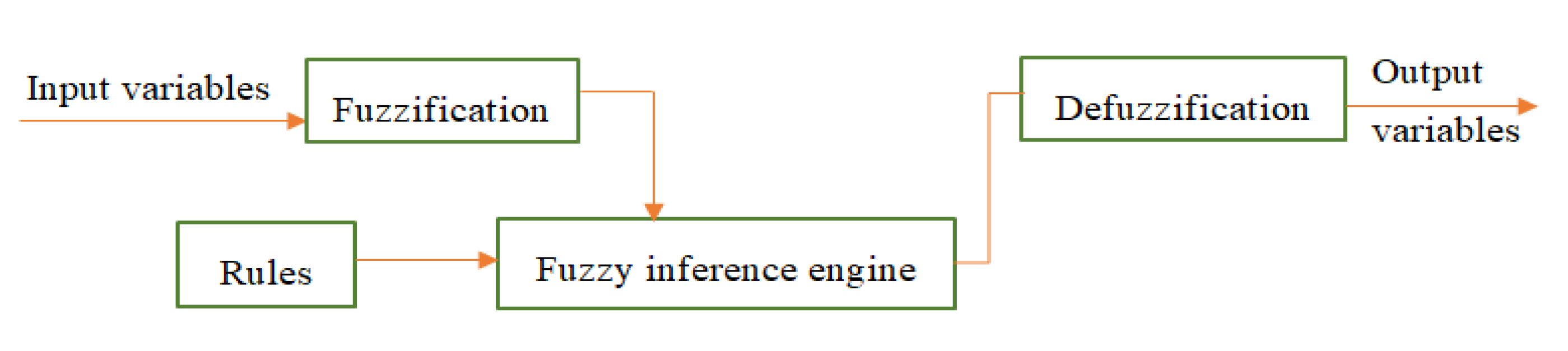The literature used to create a fuzzy logic system, starting from the definition of variables, through the rule base, and up to the defuzzification of one value from the output variable, is the book [22] and the paper [24]. Mat lab and Fuzzy Toolbox will be used to create and implement a fuzzy logic system. The basic elements of the fuzzy logic system, as well as the process of creating that system, are shown in Figure 4.

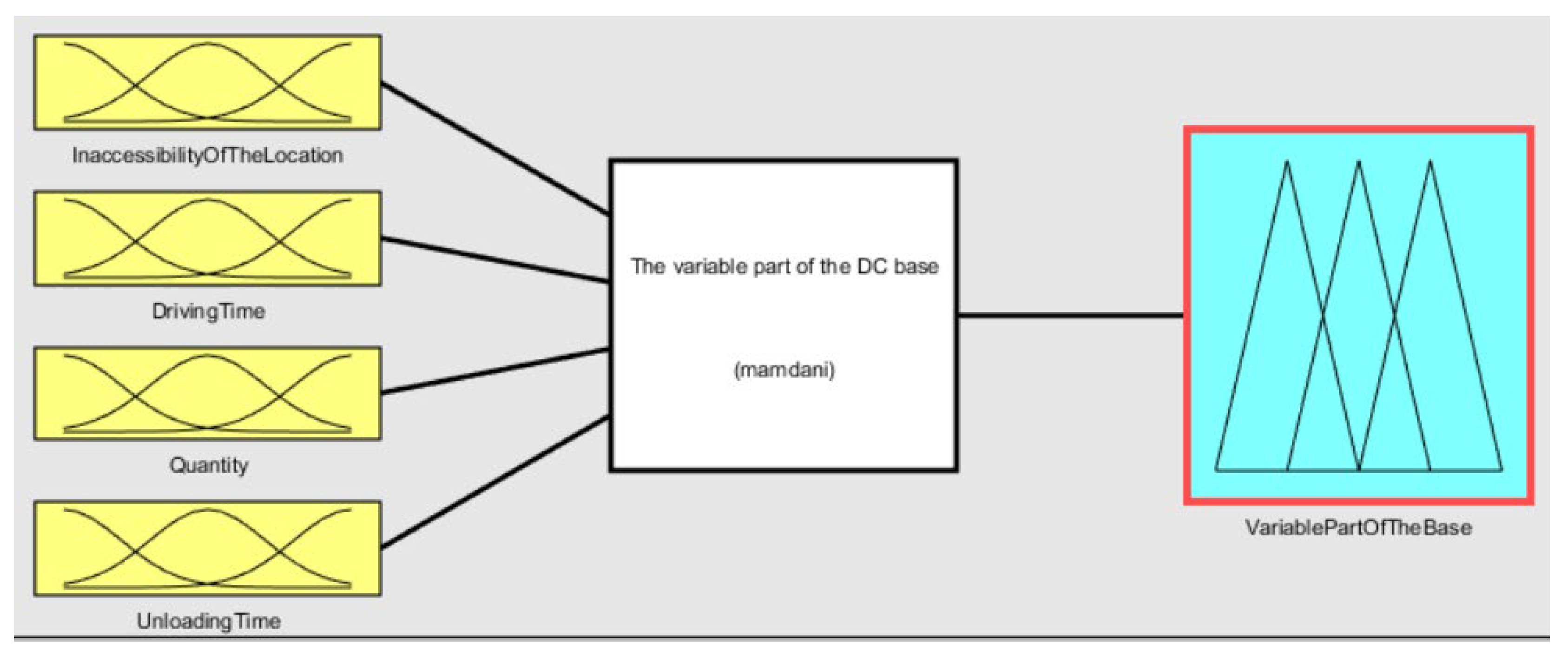
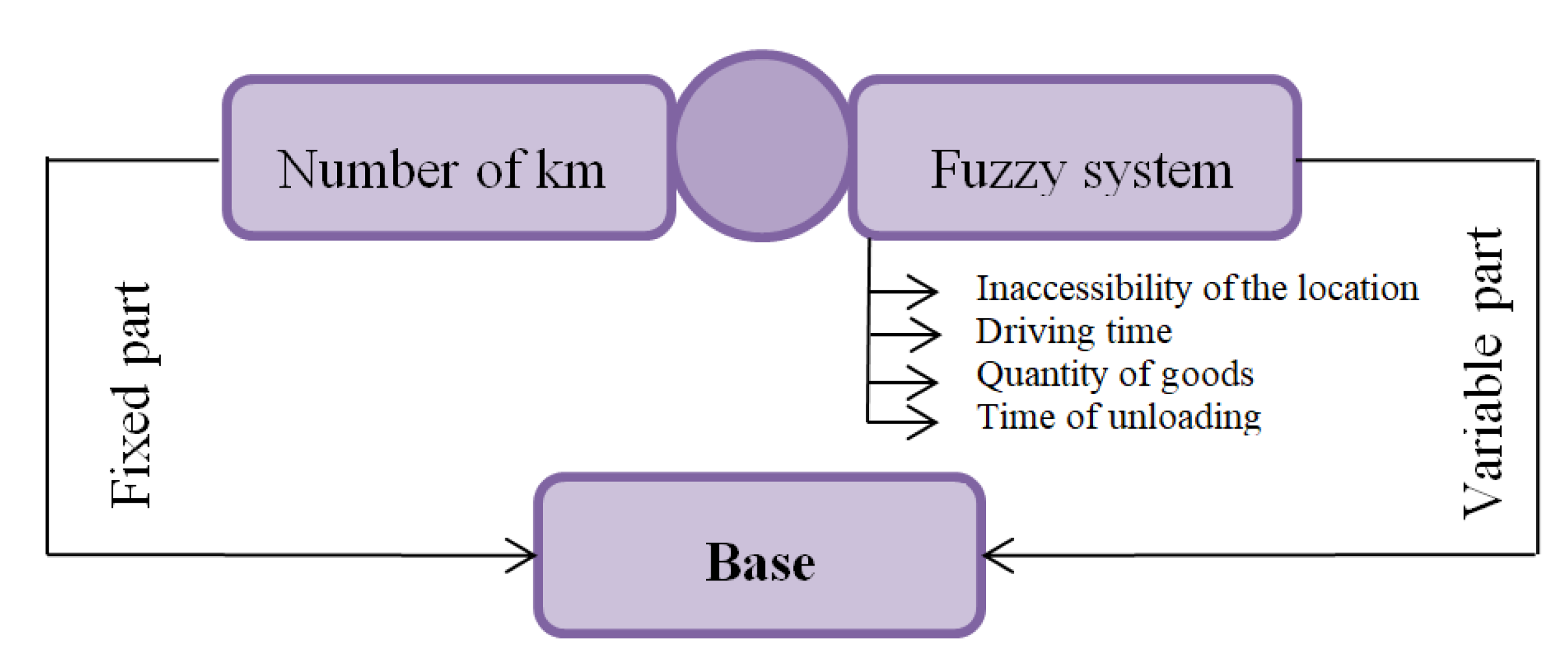
In the beginning, it should be noted that the fuzzy logic will be used to calculate the variable part of the distribution price, while the fixed part will depend only on the distance and the price per kilometer traveled, which can be seen from the scheme shown in Figure 5. The variable part determined by the fuzzy logic depends on four criteria: inaccessibility of the client’s location, driving time, quantity of goods, and unloading time. The idea is that the fixed part of the distribution price is determined before the distribution is realized, and that the additional value calculated using fuzzy logic is added only after the service has been realized. The reason for this is that, for example, the driving time may vary depending on the road conditions, so it will not always be the same for the same delivery. Also, the loading and unloading time depends on the number of pallets being transported, as well as the weight of those pallets, the sensitivity of the goods, etc. so that is also a criterion that cannot be determined in advance. The reason for taking this criterion into account is that the model is formed to determine the price of distribution to vehicles equipped with an unloading crane. In the case of using vehicles that do not have the possibility of unloading, this criterion can be neutralized by setting the value for the unloading time to 0. Customer availability is a criterion that can only be determined after the delivery has been made and is evaluated by the driver. The criterion of the quantity of goods is the only criterion from the fuzzy logic model that can be determined before the realization of the service. The model created in this way is suitable for application today due to the COVID-19 pandemic, the war in Ukraine, and other events in the world that affect the instability of the market. Nowadays, the price of fuel changes on a daily basis, so the idea of this model is that the fixed part of the base allows for a simple correction of the price of transportation due to an increase or decrease in the price of fuel. In this way, both the fixed and variable parts of the distribution price base achieve great flexibility and adaptability to newly emerging situations on the market, as well as during the realization of the distribution service.

Calculating the distribution price in this way considers the stochasticity that is very present in practice, which leads to the fact that two identical deliveries can have a different distribution price due to different conditions in which they were realized. This is the main advantage of this model compared to other models available in the literature. The base used to determine the distribution price is calculated as given by Expression (1), where the first part of the expression is fixed and the second part is variable.

O = F + V = S + c₀ + c_f,

(1)

O—basis for calculating the distribution price

F—fixed part of the base

V—variable part of the base

S—distance traveled during the realization of the distribution

c₀—transport price per kilometer traveled [€/km]

c_f—variable part of the base for the distribution price obtained based on the fuzzy logic system (€)

3.1. Input Variables

The first step in applying fuzzy logic is to define the input and output variables for the defined problem. The cost of distribution can be affected by numerous factors, some of them having a greater and some smaller influence. The biggest influence on the cost of distribution, in addition to the distance traveled, are the factors chosen as input variables, already mentioned at the beginning of this chapter:

• Inaccessibility of the client’s location;
• Driving time to the client;
• Quantity of goods;
• Time of unloading goods.

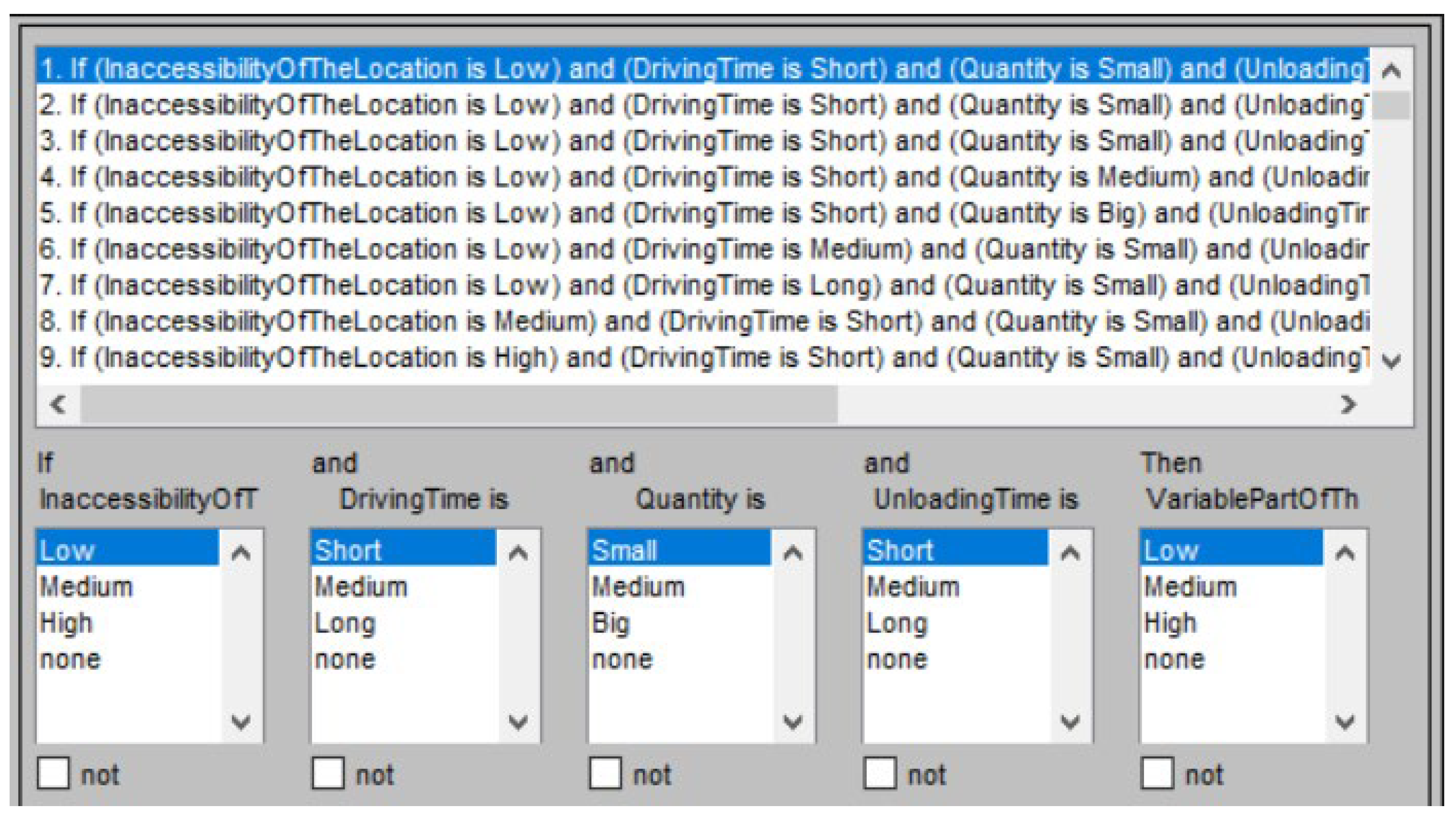
Figure 6 shows what the defined fuzzy logic system for determining the price of the distribution service looks like. From the figure, it can be seen that the four input variables listed above are defined, which determine the variable part of the distribution price base, which is the output variable.

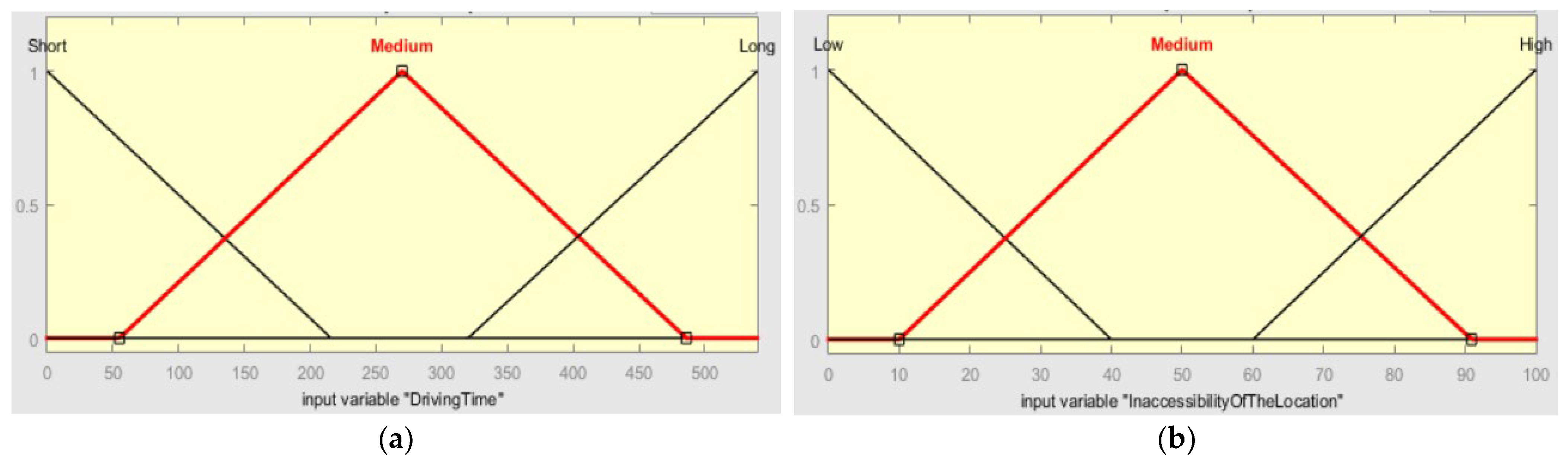
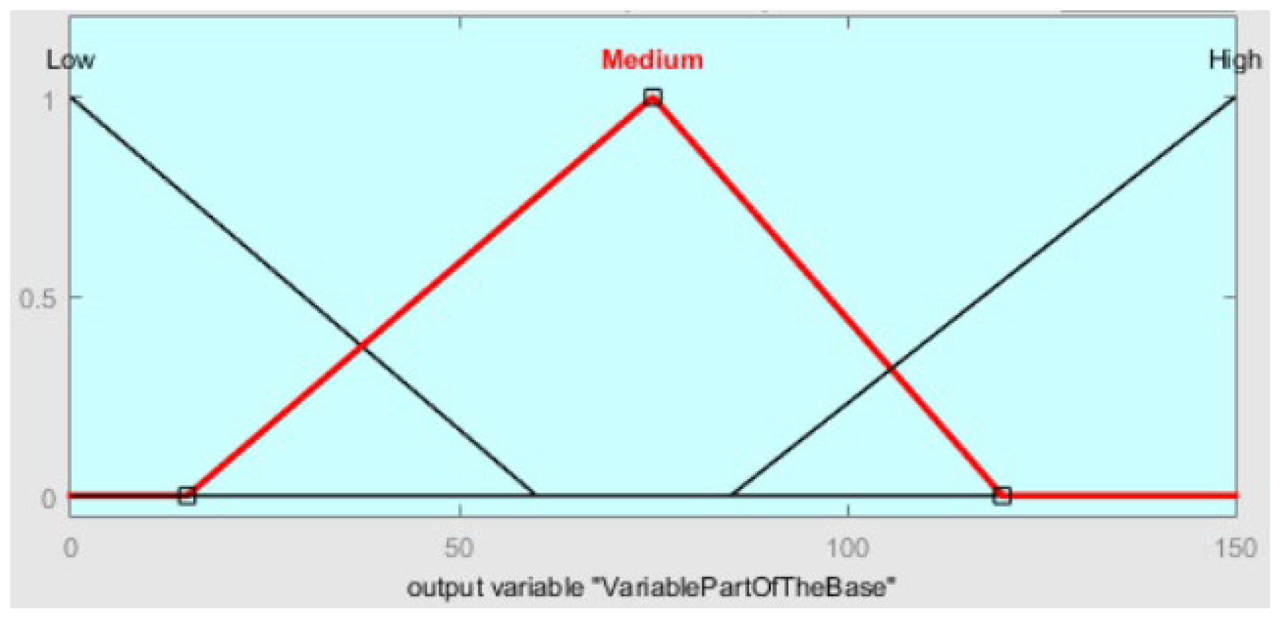
In Figure 7 (below), all four input variables are shown. The model was tested on triangular and trapezoidal fuzzy numbers. Testing on examples from practice led to the conclusion that the model works better when triangular fuzzy numbers are used. In case the model is applied in practice, the model can be updated by introducing a greater number of membership functions to make the model work better. For the purposes of this paper, during testing, the model proved to be good enough with three membership functions for each of the variables. The first input variable is the inaccessibility of the client’s location. The inaccessibility of the client’s location depends on whether he is in the city center or on the outskirts, in a hilly area or the plains. The domain of the first input variable ranges from 0% to 100%, where 100% indicates high inaccessibility to the client location and 0% indicates low. Due to the inaccessibility of the client’s location, when distributing goods, their price also increases. The main reason for this is the fact that vehicles in the central parts of the city move following the “start-stop” principle, and in this way, besides consuming more fuel, depreciation is also higher. The situation is similar when the client is on a hill or mountain, so the vehicle consumes more fuel due to the climb, as well as the brakes when braking. The location of the client as an input variable is represented by three triangular fuzzy numbers. The domain of the first input variable is divided into three intervals. The first fuzzy number is represented by the membership function called “low inaccessibility” and it is defined on the interval from 0% to 40%. The highest degree of belonging to the membership function “low inaccessibility” occurs if the distribution is made to a client whose location is rated with low inaccessibility of 0% (client on the outskirts of the city in the plain) and then it amounts to one. The membership function “medium inaccessibility” is defined on the interval from 10% to 90%. The degree of belonging to the “medium inaccessibility” function is one if the distribution is made to a client whose location is rated as 50% inaccessibility. The third membership function “high inaccessibility” is defined on the interval from 60% to 100%.

The second input variable is driving time and its domain ranges from 0 to 540 min. The driving time, i.e., the duration of the distribution, can be affected by numerous factors and it can very often be longer than planned. This happens in case of congestion, when the delivery is made in the so-called “peak hours”, when the vehicle breaks down, or in a similar situation. The longer the distribution process, the higher the distribution price, given that the driver’s working hours are longer and that the given vehicle is occupied (that is, it is not free for other clients). From Figure 7b, it can be seen that the driving time as the second input variable is represented by three triangular fuzzy numbers, the same as in the case of the previously described variable. The domain of this variable is also divided into three intervals. The first fuzzy number is represented by the membership function called “short time” and it is defined on the interval from 0 to 216 min. The membership function “mean time” is defined on the interval from 55 to 486 min. If the distribution lasts 270 min, the degree of belonging to the “mean time” function is one. The third membership function “long time” is defined on the interval from 320 to 540 min.

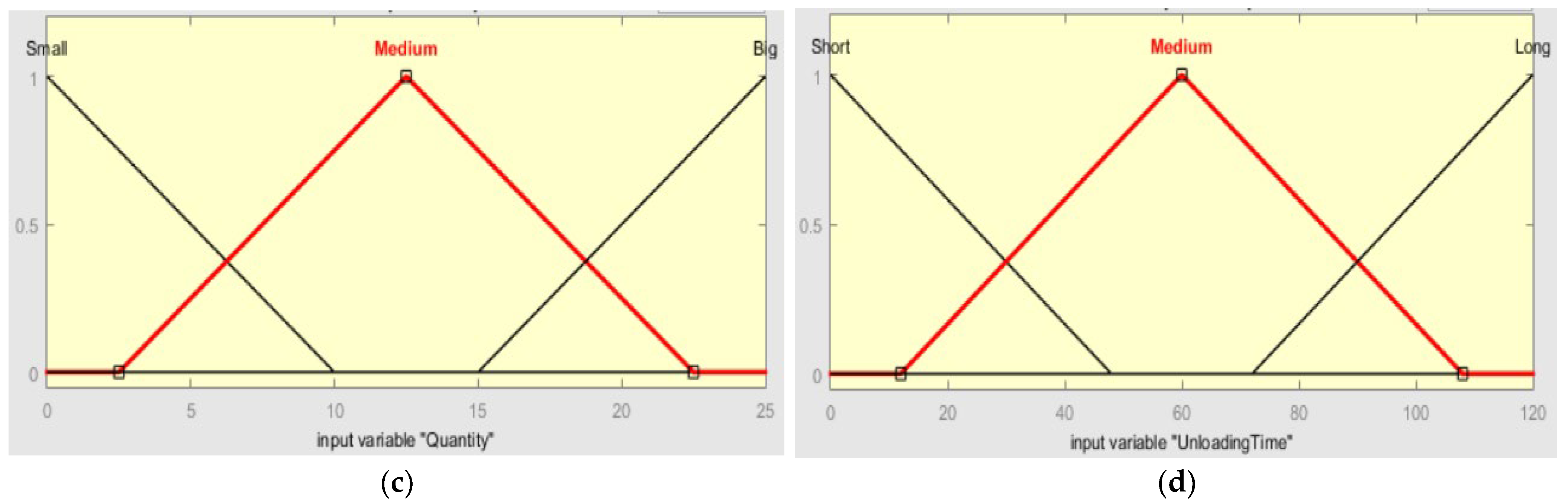
The third input variable is the amount of goods and its domain ranges between 0 and 25 tons, according to the maximum carrying capacity of the semi-truck. This variable depends exclusively on the client and his need for a certain amount of goods. The higher the quantity of goods, the higher the cost of distribution. The reason for this is, first of all, that a larger quantity requires vehicles with a higher load capacity, and these vehicles cause higher costs (they consume more fuel, and the costs of maintenance and registration are higher). Also, a larger quantity of goods for one client decreases the capacity of the cargo space, therefore decreasing the possibility to transport goods for some other clients in the same tour. This is another reason why the price increases as the quantity increases. Like the previous two input variables, the quantity of goods is also represented by three membership functions that have a triangular shape, which can be seen in Figure 7c. The first fuzzy number is represented by the membership function called “small amount” and it is defined on the interval from 0 to 10 t. The membership function “medium amount” is defined on the interval from 2.5 to 22.5 t. If 12.5 t of goods are transported, the degree of belonging to the “medium quantity” function is one. The third membership function, “large quantity”, is defined on the interval from 15 to 25 t.

The fourth input variable is the time it takes for the goods to be loaded or unloaded at the end user’s place. This time depends on several factors. First of all, it depends on the amount of goods, but also on the equipment used, the type of goods, the position of the place where the goods are unloaded, etc. This variable is important because longer loading/unloading times increase the cost of distribution. This is a consequence of the fact that the longer unloading or loading takes, the longer the vehicle and equipment are occupied, and the driver’s working hours are longer. The domain of this input variable ranges from 0 to 120 min. From Figure 7d, it can be seen that the input variable, loading/unloading time, is represented by three triangular membership functions. The first membership function “short time” is defined on the interval from 0 to 48 min. The second membership function is “mean time”, and it is defined on an interval from 12 to 108 min, and the highest degree of belonging to this function is if the loading/unloading time is 60 min when it has a value of one. The third membership function is defined on the interval from 72 to 120 min and is called “long time”.

3.2. Output Variable

After the domains are defined and divided, as well as the membership functions for each input variable, it is necessary to do the same for the output variable. The output variable is the value that should be added to the fixed part of the base, which was calculated only based on the distance traveled and the cost of transport per kilometer traveled. The domain of the output variable ranges from EUR 0 to 150 and, as with the previous variables, it is divided into three intervals and described using three membership functions, which can be seen in Figure 8. The maximum value of the variable part of the base is taken as the right border of the domain and is EUR 150. The first membership function is called “low price” and it is defined on the interval from EUR 0 to 60. The second membership function is called “mean price” and it is defined on the interval from EUR 15 to EUR 120. The degree of belonging to the “average price” function has a value of one if the variable part of the base is EUR 75. For a supplement greater or less than EUR 75, the value of the membership degree decreases, up to a price of 15, that is, EUR 120 when the membership degree is 0. The membership function called “high price” is defined on the interval from EUR 85 to EUR 150.

3.3. Formation of the Fuzzy Rule Base

When the input and output variables, their domains, and membership functions are defined, the next step is to create a fuzzy rule base. To solve the concrete problem, an exclusively expert approach was used to define “if-then” rules. Rules can be defined using the link and/or. Also, for each rule, a weight is determined that refers to the importance of the defined rule and can be in the range from 0 to 1. To solve the problem of determining the price of the distribution service, it is necessary to define 81 different rules. This number is the result of four input variables—four fuzzy numbers and three membership functions within each fuzzy number. Namely, the required number of fuzzy rules is obtained by exponentiation of the total number of membership functions by the total number of variables, i.e., 3⁴ [22]. By creating a fuzzy rule base that has 81 defined rules, every possible scenario is covered. Figure 9 shows the fuzzy rule base created to solve the problem.

3.4. Additional Factors Affecting the Cost of Distribution

In addition to the mentioned input variables, three more factors cannot be represented by a fuzzy number and must be considered when determining the distribution price. These are the type of vehicle used to transport the goods, the service quality, and the type of goods being transported. These parameters will be considered through a coefficient defined according to the importance and impact of a given parameter on the distribution price. All the coefficients from

Table 1. Factors, groups within factors, and coefficients.

Factors	A Group within Factors and Assigned Coefficients
Type of vehicle	Van			Truck			Semi-truck
	0.65			0.35			0
Quality of service	1	2	3	4	5	6	7	8	9
	−4%	−3%	−2%	−1%	0%	1%	2%	3%	4%
Type of goods	Perishable			Special handling			Sensitive to moisture
	0.2			0.1			0.05

were defined by experts, based on the experience of employees in company “X”. The idea is to multiply the corresponding coefficient with the calculated basis of the distribution price according to expression (1). The resulting value is added to (or subtracted from) the calculated base, to obtain the final price of the distribution service. Table 1 shows the factors, the groups formed within those factors, and the coefficients belonging to them.

The first factor that is very important and should have an impact on the distribution price is the type of vehicle. The reason for this is that the type of vehicle used for distribution directly affects fuel consumption, and therefore should also affect the price of distribution. With this factor, it is defined that from the base, that is, from the price calculated after adding the variable part given by the model, it is necessary to subtract the value obtained by multiplying the base with the coefficient. This is defined due to the assumption that the base is calculated for distribution carried out by semi-trucks. In such a situation, when a semi-truck is used, the coefficient is 0 and there will be no basis reduction. However, when smaller vehicles are used, fuel consumption is also lower, so the cost of distribution should be lower. For this reason, the coefficient is 0.65 for vans and 0.35 for trucks. The coefficients are defined proportionally with the consumption of vehicles of that type, and if it is considered that the truck consumes 35% less fuel compared to the semi-truck, then the basis must be reduced by the amount of the basis*0.35. It should be noted that this factor considers the driver’s labor costs, as well as vehicle maintenance costs. Namely, driving larger vehicles such as a semi-truck requires more qualified drivers compared to vans and solo trucks, so the distribution price should be different. Likewise, the maintenance of semi-trucks and solo trucks is much more expensive compared to vans in terms of more expensive equipment (tires and other parts), more expensive vehicle registration, more expensive repairs, and the like.

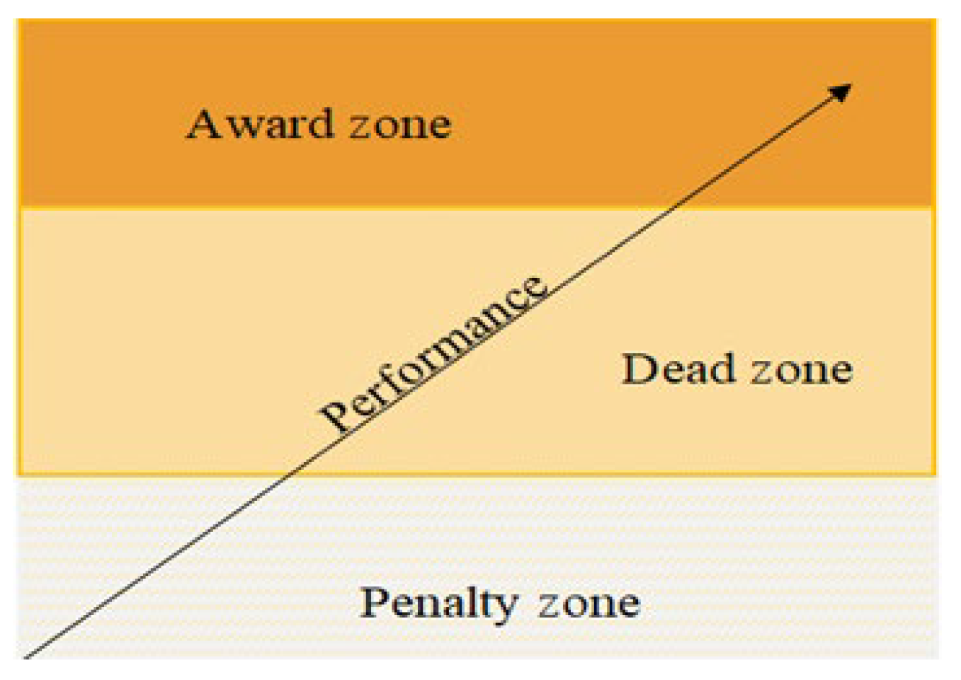
An essential part of the distribution price should be the quality of the service. Quality should be included in the price in such a way that if the distributor does his job properly, he will be rewarded for it, or if he is not, he will be punished. For example, if the distributor respects the client’s time windows, delivers the right goods to the right place, or in some way increases the value of the service to the end user, then he should be rewarded by increasing the distribution price. Conversely, if there is a delay in delivery, if the goods are damaged in transit, or if the distributors deliver the wrong goods, then they should bear the consequences by reducing the cost of distribution. Accordingly, the service quality factor can be rated from 1 to 9. The customer is obliged to rate the quality of the service after each realized distribution service. In this way, the distributor receives an average rating for the quality of his services, based on which he has the right to charge more or less for his service. If his average score is less than 5, the distributor will be obliged to charge less for his service, and if his service has an average score higher than 5, he has the right to increase the total price of the distribution of goods. The final price of the distribution service is obtained when the calculated value is increased or decreased by the corresponding percentage from Table 1, depending on the average score that the distributor has on the quality account.

The quality of the service will be included in the price of distribution and through penalties that distributors pay in the case of deviations. This approach is most often used in practice, and that is why, in the case of some irregularities, the quality factor is best considered through the aforementioned penalties [1]. The proposal is that in the case of certain defects, the distribution price is reduced by 10–30%. The percentage of the price reduction depends on how much the deviation affects the client and his further workflow. Some of the deviations are delivery delays, damage during delivery, lack of documentation, and the like. On the other hand, if the distributor does not deliver the goods to the client, the client is not obliged to pay the distribution contractor, i.e., the penalty is 100%. The most common penalties that reduce the cost of distribution by 10–30% are [25]: unjustified delay to the place of loading more than 60 min, unjustified delay to the place of loading more than 30 min (when it comes to a meat, fruit, and vegetables warehouse), failure to arrive at the place of loading, late invoicing or incorrect invoice, non-delivery of route documentation by the service provider, behavior of the driver deviating from the contractual obligations, delay in returning packaging for meat-containers and ships by 7:00 p.m., non-receipt of return packaging at the facility-pallets, ships, and others, non-compliance with transport conditions related to HACCP regulations

When it comes to the factor of the type of goods, for the developed model, three categories of goods will be considered: perishable goods, goods that require special handling, and goods sensitive to moisture. Perishable goods include foods such as milk, meat, eggs, fish, and the like. The mentioned goods are transported in refrigerators that provide them with the appropriate temperature regime. Refrigerators belong to a type of vehicle that is very expensive from the distributor’s point of view in terms of fuel consumption, but also maintenance. Refrigerators for the transport of perishable goods must work non-stop and maintain the temperature during transport, so the fuel consumption is much higher compared to classic vehicles, and therefore the cost of distribution. Namely, even when the driver takes a break of 11 h, the refrigerator must work for all 11 h, so that the product does not spoil. In the case when the transport of perishable goods takes up to 9 h, then the distribution price must be increased by using a coefficient of 0.2. On the contrary, if the transport lasts more than 9 h and includes the mentioned break of 11 h, then the distribution price needs to be additionally increased by the amount of the costs of operating the cold store during those 11 h.

As for goods that require special handling, this includes dangerous, expensive, and breakable goods. Unlike the previous one, ordinary vehicles are used in this category, so the distribution price does not need to be increased due to fuel consumption. The main reason for the increase in the distribution price for this category of goods is the greater responsibility of the transport company. There are much greater risks when transporting the mentioned types of goods than in the case of ordinary goods. If some expensive goods are being transported, there must be adequate protection in the form of an alarm to prevent theft, and this requires additional costs for the carrier. Also, if some dangerous goods are being transported, it requires special caution and a way of handling them so that there are no explosions and other unwanted consequences. Due to the aforementioned facts, the coefficient 0.1 will be used for goods that require special treatment to increase the distribution price.

The third category includes goods that are sensitive to moisture, such as building materials, wheat, barley, and corn. These types of goods do not require a special temperature regime, but only to protect the goods from weather conditions by placing a tarpaulin. In that case, putting a tarpaulin increases the weight of the vehicle, and thus the fuel consumption, so it is necessary to increase the cost of distribution. Given that the consumption is much lower compared to a refrigerator, and the risk is much lower compared to goods that require special treatment, then for goods that are sensitive to moisture, a coefficient of 0.05 should be used to increase the distribution price.

It should be noted that the aforementioned division into three categories was made for the developed model for calculating the distribution price. Since there are many different types of goods, it is possible to make a much more detailed and precise classification in the case of developing some more complex models for calculating the distribution price. As before, the distribution price in the case of a certain type of goods is increased by adding to the base the amount obtained by multiplying the base and the corresponding coefficient.

4. Testing the Fuzzy Logic Model on Hypothetical Data

In the previous chapter, a fuzzy logic system was created, which aims to determine the variable part of the distribution service price base. The created model must be tested on a sufficiently large number of cases for its validity to be confirmed. This means checking the way the model “behaves” and the solutions it gives when different input variables are entered. According to experts, if the model gives good output results for various scenarios, then it can be considered valid according to experts. However, practice has shown that it is the best to use the model created in this way as a pilot project, and then work on its improvement during use. It is also possible to determine the efficiency of the model created in this way by applying the DEA method, as was done in the paper [5], in which the DEA method was used to determine the efficiency of the distribution center’s operations.

The model was first tested on hypothetical examples generated by experts in this field. The test cases are generated in such a way as to cover the largest number of cases that may arise in practice when providing a distribution service. When determining the distribution price, it is first necessary to calculate the value of the fixed part of the base, and then, by applying the created fuzzy logic system, calculate the variable part of the base, which depends on the availability of the client’s location, driving time, quantity of goods, and loading/unloading time. To obtain the final price of distribution, it is necessary to consider other factors, namely the type of vehicle, the quality of service, and the type of goods, through the assigned coefficients. The created model was tested on a total of 12 scenarios, for which it gave fairly good results. The obtained results, i.e., fixed and variable parts of the base, for all 12 scenarios will be shown in

Table 2. Test results.

Scen.	S [km]	F [€]	Values of Input Variables				V [€]	Res.
			Customer Location [%]	Time [min]	Quantity [t]	Time of Unloading [min]		O [€]
1.	30	60	70	80	3	15	42.7	102.7
2.	110	220	80	120	7	35	75.3	295.3
3.	105	210	10	150	24	45	59.1	269.1
4.	95	190	60	100	2	25	45.7	235.7
5.	35	70	90	70	3	18	40.7	110.7
6.	240	480	30	360	19	40	73.6	553.6
7.	18	36	65	40	2	20	37	73
8.	74	148	20	95	6	26	50.3	198.3
9.	80	160	30	105	17	26	61.2	221.2
10.	22	44	75	35	2.5	22	48.5	92.5
11.	140	280	85	215	7	25	78.3	358.3
12.	120	240	20	180	23	45	64.4	304.4

.

Once the distribution price base is calculated, it is necessary to include other important factors to obtain the final price of the distribution service. Factors related to the type of vehicle, quality of service, and type of goods will be included in the price through previously defined coefficients in Chapter 3. The final distribution price will be calculated according to the following Expression (2):

CD = O ± O × COEFFICIENT,

(2)

CD—the cost of distribution service.

It should be noted that an amount is added to the base, i.e., a + sign is used in the case of the quality factor when the service provider has an average rating for quality higher than 5 and in the case when the goods fall into one of the three defined categories. In those situations, the factor will increase the cost of distribution. However, if the quality score is less than 5, the distribution price will be reduced. On the other hand, the amount is subtracted from the base, i.e., the “−” sign is used in the case of the vehicle type factor. As already mentioned, this happens since the base is formed for the type of semi-truck.

Table 3. The final cost of distribution.

Scen.	Factors			Result
	Type of Vehicle	Quality of Service	Type of Goods	Cost of Distribution [€]
1.	Van	5	Special handling	46.21
2.	Truck	7	Perishable	251
3.	Semi-truck	3	Without a request	263.71
4.	Van	1	Perishable	120.2
5.	Truck	9	Without a request	75.27
6.	Semi-truck	7	Sensitive to moisture	592.3
7.	Van	9	Without a request	28.47
8.	Truck	2	Without a request	122.94
9.	Semi-truck	4	Perishable	263.22
10.	Van	6	Without a request	33.29
11.	Truck	8	Special handling	279.47
12.	Semi-truck	5	Without a request	304.4

will show other factors and the final cost of distribution for each scenario. Out of a total of 12 scenarios, the first scenario will be described in more detail below.

In the first example, it is assumed hypothetically that 3 tons of certain goods need to be distributed over a distance of 30 km. At the same time, the transportation of those goods lasted 80 min, while the unloading operations lasted 15 min. The mentioned parameters are at the same time the values of the input variables for the created fuzzy logic system, and the distance parameter is the input for calculating the fixed part of the base. Defuzzification, i.e., obtaining a single value from the output variable, was realized using the center of gravity method. To the obtained fixed part of EUR 60, it is necessary to add the variable part of the base of EUR 42.7, which gives a fuzzy logic system.

However, the resulting price of EUR 102.7 is not the final distribution price. To arrive at the final price, it is necessary to include the factors of type of vehicle, quality of service, and type of goods. In the specific example, a van is used for the transport of goods, where the distributor has a service quality rating of 5, determined based on previously performed services, and the type of goods being transported belongs to the group of goods with special handling requirements. Given that it is a van, i.e., a vehicle that achieves the lowest fuel consumption, its basis must be reduced using a coefficient of 0.65. On the other hand, as the distributor has a score of 5 for quality, this parameter will not affect the cost of distribution, because the coefficient assigned to the score of 5 is equal to zero. Since the goods being transported have special handling requirements, it is necessary to increase the base using a coefficient of 0.1. During the realization of the delivery, there were no major irregularities, so the distributor will not pay any penalties. Therefore, the final distribution price is CD = EUR 46.21 and was obtained as follows: CD = 102.7 − (102.7 * 0.65) + (102.7 * 0) + (102.7 * 0.1) = EUR 46.21.

The cost of distribution for the remaining 12 scenarios is determined in the same way as for the first one, which is explained in detail. Depending on the vehicle, quality rating, and type of goods, the base is increased or decreased following the assigned coefficients.

5. Sensitivity Analysis of the Fuzzy Logic Model

To confirm the validity of the created model, a sensitivity analysis of the fuzzylogic system was also performed in this paper. The goal of sensitivity analysis is to identify the most sensitive input variable of the fuzzy logic system, whose change has the greatest effect on the output value. The sensitivity analysis was performed in such a way that the value of each of the input variables was increased first by 10%, and then by 30%. Also, the sensitivity analysis was performed when the values of the input variables were reduced by 10%, and then by 30%. Based on the described changes in input values, it was analyzed how the output value of the fuzzy logic system changes.

Table 4. Sensitivity analysis.

Scen.	Input	Input Values	V [€]	V [€] Input Increase by 10%	V [€] Input Increase by 30%	V [€] Input Decrease by 10%	V [€] Input Decrease by 30%	V [€] Average Change
1	Customer location [%]	70	42.7	45.3	48.4	40	35.4	4.575
	Time [min]	80	42.7	45.4	49.5	39.4	32.5	5.75
	Quantity [t]	3	42.7	43.8	45.5	39.8	37.8	2.925
	Time of unloading [min]	15	42.7	42.7	45.6	40.8	37.8	2.425
2	Customer location [%]	80	75.3	75.5	75.9	74.2	59.4	4.45
	Time [min]	120	75.3	78.1	82.8	72.8	67.4	5.175
	Quantity [t]	7	75.3	76.8	81.4	75.1	72.5	2.65
	Time of unloading [min]	35	75.3	75.5	75.8	74.4	72.4	1.125
3	Customer location [%]	30	73.6	73.6	78.4	73.6	73.2	1.3
	Time [min]	360	73.6	81.3	84.2	65.4	63.4	9.175
	Quantity [t]	19	73.6	73.7	78.1	73.2	64.4	3.55
	Time of unloading [min]	40	73.6	76.5	79.1	70.5	70.1	3.75

shows three examples for which the output value of the fuzzy logic system, which represents the variable part of the distribution price base, was determined. From Table 4, it can also be seen how the output value of the model increases or decreases as the value of each of the input variables changes. In the first example, the inaccessibility of the location was assessed as 70%, the transport time was 80 min, the amount of transported goods was 3t, and the unloading time of the goods lasted 15 min. For the described example, the variable part of the distribution price was 42.7e. In the following columns of the table, it can be seen how the output value of the model is changed by changing each of the input variables individually. For example, by increasing the value related to the inaccessibility of the location by 10%, the variable part of the distribution price base increases from EUR 42.7 to EUR 45.3. Extending the transport time by 10% leads to an increase in the variable part of the distribution price base from EUR 42.7 to EUR 45.4. In this example, the input variable quantity is less sensitive to a change in value than the previous two variables. An increase in the quantity transported by 10% increases the variable part of the distribution price base from EUR 42.7 to EUR 43.8. Regarding the input variable unloading time, it can be said that in the case of a 10% increase in value, it is the least sensitive, because it does not lead to a change in the output value of the model. Also, for the first example, Table 4 shows the changes in the output value of the model in three other cases: an increase in the value of each of the input variables by 30%, a decrease in the value of each of the input variables by 10%, a decrease in the value of each of the input variables by 30%.

To be able to compare the input variables from the aspect of their influence on the output value, the average change in the output value was determined for each input variable. The average value of the change in the output value for a specific input variable is determined based on four different magnitudes of change in the input variable. In this way, it can be seen from Table 4 that the average change in the output value of the model in the case of a change in the value of the input variable location inaccessibility is EUR 4.5. In the same way, it was obtained that the average change in the output value of the model due to the change in the transport time is EUR 5.75, the quantity is EUR 2.9, and the unloading time is EUR 2.4. Based on the obtained results, it can be concluded that in the first example, the most sensitive input variable is the transport time, because the change in its value has the greatest impact on the variable part of the distribution price base. In the following two examples, as well as in the first one, it was found that transport time is the most sensitive input variable. Based on that, it can be concluded that it has the greatest influence on the formation of the variable part of the distribution price base. The inaccessibility of the location was identified as the second most sensitive factor, while the third most sensitive factor was the amount of transported goods. The sensitivity analysis of the model created in this paper aimed to confirm the validity of the fuzzy logic model in addition to identifying the most sensitive input variable.

6. Model Testing on the Example of the “X” Company

The originally developed model for calculating the distribution price was tested through some hypothetical examples to verify its validity. Now it is necessary to check what results the model gives when it is tested on a concrete example of a company that provides a distribution service. The testing will be carried out in the “X” company for the sale of building materials and their distribution [8]. In the following part, some basic information about the company and its activities will first be given. Then, the distribution of the company will be described, that is, how the distribution process takes place, with which vehicles, in which area, etc. Finally, the developed model will be applied to real examples of the distribution of the “X” companies. In addition, the obtained results will be compared with the price that the company charges in given situations, all to check the validity of the developed model. The paper presents examples of the distribution of goods in the “X” company which, according to experts, can best demonstrate the advantages of the created model concerning the approach applied by the “X” company.

6.1. “X” Company and Its Distribution

The “X” company for the sale of building materials and their distribution was founded in 2005 in Western Serbia, in the town of Lajkovac. This is a sales company, i.e., a warehouse of building materials, which, in addition to sales, provides the service of distribution of its goods, as well as those of others. Some of the basic materials sold by this company are cement, lime, tiles, timber, pellets, blocks, bricks, pipes, sheets, sand, gravel, and more. The company has its vehicle fleet for transporting goods, as well as transshipment machinery for loading and unloading them. Also, the goods are stored in their premises, whereby part of the goods that are not sensitive to moisture and weather are stored outdoors, while the other part of the goods that are sensitive to moisture are stored in a closed part of the warehouse. As for the employees, the company operates successfully with only four employees, two of whom are the owners of the company. One employee does long-distance procurement and distribution, another does daily distribution in the area, the third is at the warehouse and issues goods, i.e., he is in charge of loading/unloading goods, and the fourth sells goods and is responsible for documentation.

As previously mentioned, the company provides the service of distribution of its own and other parties’ goods. As for the area where the distribution is carried out, there are no spatial restrictions, although the most common deliveries are to the surrounding towns and villages near Lajkovac (“X” depot). However, there are also frequent deliveries to Kikinda, Beočin, and Kosjerić, where return tours are usually organized to deliver construction materials to the warehouse.

Deliveries are made by company vehicles. The company owns two semi-trucks with a carrying capacity of up to 25 t, which are used on long distances, one of which is a MAN brand, and the other is a SCANIA brand. Two DAF and MAN trucks are used for transporting goods up to 7 tons, both of which have a crane that is used for loading and unloading goods. For shorter distances, the Opel Kadet pickup truck is used for goods with a load capacity of up to 1t. The distribution is carried out by two qualified drivers, one of whom makes deliveries on shorter distances, with vehicles of smaller capacity, while the other is in charge of transporting goods with semi-trucks (“X” warehouse).

It should be noted that the company has different semi-trailers at its disposal and that the choice of a semi-trailer to be placed on the semi-truck depends on the type of goods being transported. Namely, open semi-trailers transport goods that are not sensitive to the weather, such as bricks, blocks, roof tiles, and the like. On the other hand, a closed semi-trailer or a semi-trailer with a tarpaulin is used in the case of sensitive goods such as cement, pellets, and lime. In addition to two semi-trailers (with and without tarpaulin), the company also has one multi-purpose semi-trailer that can tip and can also transport palletized goods. This semi-trailer allows bulk goods to be transported in one direction and palletized goods in the other direction.

6.2. Method of Calculating the Distribution Price in the “X” Company

When it comes to the distribution price, the company calculates in two ways depending on the situation. The first way is through the application, which takes into account the location of the delivery, the mileage covered, the origin of the goods, and the number of pallets transported. Another way of calculating the price implies that the base is multiplied by the number of kilometers traveled, to which are added the costs of unloading (if any). The basis is 120 dinars/km (1 €/km), and it is the same in both directions, that is, whether the truck is going full or empty. This way of calculating the price is used in some situations, for example when the application does not work or it is necessary to calculate the price outside the point of sale. Figure 10 shows the layout of the application used by the company, followed by an explanation of it.

When entering the application, the distributor has the option to choose whether it is a matter of transporting goods to a new or an existing location. The existing locations are those that are frequently used and can be seen in Figure 10. Own goods are only transported to these locations, with the option to select the number of pallets to be transported. This information is important for unloading operations. In the case when up to three pallets are transported, the model takes one unloading price, and in the case when more than three pallets are transported, another price. If you choose a new location at the beginning, you must first enter the name of the place and the number of kilometers. This is followed by the selection of the origin of the goods being transported, i.e., whether they are your own or customers, as well as the number of pallets. If the customer’s goods are transported, the cost of distribution will be higher than in the case of own goods. It should be noted that the company’s model was created in such a way that it immediately calculates the cost of transportation for the total kilometers traveled, i.e., in both directions of travel.

It can be concluded that when calculating the distribution price, the company takes into account the origin of the goods, the number of pallets, and the mileage traveled. As a disadvantage of the currently used model, it can first be noted that it does not consider the vehicle load, i.e., the amount of goods being transported. The fact that the type of goods being transported is not taken into account, and clients who require sensitive goods and those who need ordinary goods are treated the same are also disadvantages. Some other shortcomings are certainly the neglect of location and quality factors that are included in the newly developed price calculation model.

6.3. Testing the Developed Model on the Example of the “X” Company

This part of the paper aims to apply the previously developed model using fuzzy logic to some real situations in company “X”. The model will be tested through three examples, that is, the distribution price will be determined in three different scenarios. In doing so, completely different situations will be considered in terms of mileage, type of vehicle used, location, and the like, all to better verify the validity of the developed model.

6.3.1. Discussion 1: Distribution of Crushed Stone in Kikinda

In the first iteration, it was necessary to transport 20 tons of goods from Lajkovac to Kikinda, covering 224 km. The mentioned transport lasted 200 min, and the loading and unloading operations lasted 20 min. The above information is real and was obtained from a driver who performs distribution on the mentioned route in the “X” company. These data represent the values of the input variables for the model developed in this paper. By applying the created model, it is obtained that the basis of the distribution price is O = EUR 509.7, of which the fixed part is EUR 448, and the variable part is EUR 61.7.

As before, to arrive at the final distribution price, it is necessary to include other factors that affect the price. In this case, the customer’s goods, namely crushed stone, were transported to Kikinda. For transportation, a semi-truck with a specialized semi-trailer that has the possibility of tipping was used. Also, this semi-trailer ensures that on the way back from Kikinda, palletized goods (for example roof tiles) that are needed for sale at the warehouse are returned. Since the basis of the distribution price is formed for the semi-truck, in this situation no value should be deducted from the basis. As for the type of goods, it does not affect the price in this case because crushed stone does not belong to goods that are sensitive to moisture. Since there were no complaints or damage during transport, the distribution price does not need to be reduced due to the poor quality of the service, but it is necessary to increase it due to the distributor’s quality rating, which is 8. Therefore, it can be concluded that in this example, the ultimate price equal to CD = 509.7 + (509.7 * 0.03) = EUR 524.99.

“X” company charged RSD 56,800 (EUR 483.4) for the previously described transport of crushed stone to Kikinda. It can be concluded that in this example, the model developed in this paper and the model used by the company give a price that differs by about EUR 50. Figure 11 shows the price given by the company’s model for the described example 1. It should be noted that the field related to the number of pallets was not checked because the object of transport was bulk goods.

6.3.2. Discussion 2: Distribution of Building Materials in Lazarevac (Šopić)

In the second example, it was necessary to transport 0.5 tons of goods from Lajkovac to Šopić, i.e., a place near the city of Lazarevac. At the same time, 18 km are covered, transport takes 10 min, loading and unloading takes 10 min, and the inaccessibility of the location is rated at 60%, considering that it passes through the center of the city of Lazarevac. The model created in the paper provides a distribution price basis of O = EUR 105.7, of which the fixed part is EUR 36, and the variable part is EUR 69.7.

To obtain the final distribution price, it is necessary to include all the factors that affect the price. Unlike the previous example, in this situation, the company sold its goods to the client and enabled him to deliver the purchased goods to the town of Šopić, near Lazarevac. In particular, it was necessary to transport three corrugated sheets, 30 m of lath, and 50 screws. Since the quantity of goods is smaller and the distance is shorter, the mentioned truck of the “X” company, Opel Kadett, was used for transportation. Considering the similarity between that vehicle and the van, the coefficient assigned to the van in the developed model, i.e., 0.65, will be used to reduce the base. As for the factor of the type of goods, in this case, they do not affect the cost of distribution, because the goods that are transported do not need special conditions. On the service quality account, it is necessary to increase the base by 0.03, considering that the quality rating is 8. The final price of distribution in this example would amount to CD = EUR 40.16 according to the developed model and be obtained as follows: CD = 105.7 − (105.7 * 0.65) + (105.7 * 0.03) = EUR 40.16.

In the case of transporting its goods to Šopić, the company charged 4100 dinars (EUR 34.89). As in the previous situation, the prices of the observed models differ, but not significantly, by around EUR 5. The price difference occurs because the company does not consider the factors of location and type of vehicle, but only the kilometers traveled, the origin of the goods, and the number of pallets to be unloaded. Certainly, it can be concluded that the developed model using the fuzzy logic system gives solutions very close to the real price.

6.3.3. Discussion 3: Distribution of Fodder in Kosjerić

The third example refers to the transport of 6 tons of customers’ goods from Lajkovac to Kosjerić, which covers a distance of 77 km in one direction. The transport lasted 221 min due to roadworks, loading and unloading operations 25 min, and the inaccessibility of the location was rated at 95% due to the mountainous areas to be crossed. The model created in the paper gives a base amounting to CD = EUR 237.4, of which the fixed part is EUR 154, and the variable part is EUR 83.4.

After the distribution price base is obtained, other factors need to be included to arrive at the final price. Since the goods being transported are fodder and belong to the type of goods that are sensitive to weather conditions and must not get wet, it is necessary to use a means of transport with a tarpaulin. In this case, one of the trucks with a crane is used, given that the quantity of goods is three pallets, i.e., 6 tons. Since the type of vehicle is a truck, the basis must be reduced through a coefficient of 0.35. In the previous two examples, the factor of the type of goods did not affect the price because ordinary goods were transported. Now it is a type of goods that are sensitive to moisture, so the basis should be increased through a coefficient of 0.05. As there were no complaints, damages, or delays, there are no penalties from the aspect of service quality this time either, which would affect the price reduction, except for the service quality rating, which is 8, which leads to an increase in the distribution price. If all the mentioned factors are considered, the final distribution price can be reached, which is CD = EUR 173.3, which is obtained as follows: 237.4 −(237.4 * 0.35) + (237.4 * 0.05) + (237.4 * 0.03) = EUR 173.3.

“X” company charged 20,050 dinars (EUR 170.63) for the aforementioned transport and distribution service. This once again shows that the price is approximate compared to the model using fuzzy logic. In this example, the difference between the prices is about EUR 3. In this example, the advantage of this model can be seen the most, which is its adaptability to specific situations during delivery, such as roadworks. By applying the model developed in this paper, the distribution price included a longer delivery time than expected, due to roadworks. The developed model takes into account additional factors that increased the cost of distribution, namely the type of goods and location. “X” company is advised to introduce additional factors to determine the distribution price more precisely. The reason why there is not a bigger difference in the cost of distribution is that in the model used by the company, the boxes related to the origin of the goods and the number of pallets is checked. Both data increase the price considering that fodder is being transported; other people’s goods and three or more pallets are being unloaded.

6.4. Managerial Insights

Based on the testing of the developed model for determining the distribution price on hypothetical examples, but also on examples from practice, it can be concluded that the model is very suitable for application in practice. Compared to the approach used by the “X” company, the model developed in this paper defines a price similar to the company’s model, but taking into account several factors and having the possibility to correct the price in case of some unforeseen circumstances that occur during the realization of the service.

The model developed in this paper is very suitable for application in companies from the aspect of their assurance that their costs will always be covered. Also, the model enables the generation of lower prices for users when the service is provided without unpredictable circumstances (crowds, roadworks, excessive unloading time, etc.). The developed pricing approach is very simple and very easy to apply in practice and suitable for application in conditions such as pandemics, war, and other types of disruptions when the costs of the company providing the service can vary significantly from day to day due to market crises. The only condition for the application of the developed model is that it be accepted by the users, given the existence of a certain level of uncertainty about the final price that they should pay for the received service. It is most important to explain to users that by applying this model they can obtain lower prices for the requested service in most cases (when the service is provided without unforeseen circumstances), compared to the price that would be generalized and defined by applying existing models in the literature and practice. Also, it would be necessary to build a certain level of trust between the company providing the service and the user of the service so that the users are sure that the companies will not abuse the variable part of the service price to charge a higher amount. As an advantage of the created model, it should be noted that it also takes into account the quality of the service provided, so due to a high rating for quality, the company can make extra profit, but also the user can pay for a lesser service due to poor quality.

7. Conclusions

The distribution service brings with it numerous challenges and problems. One of the basic ones, which is present every day, is the determination of the distribution price. The existing methods used for this purpose will not always give the true price that needs to be paid for this service. Such methods would lead to a situation where two clients who need the distribution of goods at different distances and at different times pay the same price because a tabular approach is used. This should not be the case, because in this way one of the clients will be harmed. By applying the fuzzy logic system for determining the distribution price, an individual price will be generated for each client and each delivery, depending on the circumstances in which the delivery was made. This was exactly the aim of this paper, with the ultimate intention to ensure equality and satisfaction of the demands of all interested parties in every situation, as well as the adaptability of the model to constant changes in the price of fuel on the market.

If we consider two clients who require distribution in the same city, but in different locations, the created fuzzy logic model will give different prices for those two clients, which would not be the case if a tabular approach were used. Also, two similar deliveries for the same client may have a different price that depends on road conditions, i.e., driving time due to some unexpected situations, inaccessibility of the client due to possible crowds, and unloading time in case of specific client requests. Accordingly, it can be said that the developed model is better compared to the previously used methods of price calculation because it more accurately determines the price of distribution and ensures equal treatment of each client. Likewise, the tests that were performed in the fourth and fifth chapters of the paper showed that the model is valid considering that it gave quite realistic solutions for the given hypothetical situations. Testing on a real example of the “X” company showed that the model can be applied in the field of distribution and that it gives prices that are very realistic and much more precise than those charged in practice.

Although there was a tendency in the paper to consider most of the criteria that are important for the price and to improve the model as much as possible, it can be concluded that the disadvantage of the created fuzzy logic system is that this model does not consider all possible factors that influence the cost of distribution. For this reason, if a company intends to implement this model in its business, it is first recommended that it be introduced as a pilot project. After the introduction of the pilot project, further improvement of this model would be carried out in terms of corrections of currently defined intervals, definition of new membership functions, or introduction of new variables that are determined to have an important impact on the price.

The scientific contribution is that there are no similar works in the literature based on these inputs (inaccessibility of location, delivery time, quantity, and unloading time), and precisely these corrective factors (type of vehicle, quality of service, and type of goods) that are developed for real logistics systems. Also, the contribution of this paper is that a unique approach to the formation of the distribution price has been developed in two parts, before the realization of the service and after the realization of the service. By applying this model, companies do not have to include unpredictable costs in the distribution price, which allows them to offer a lower price and thus be more competitive in the market. Another contribution of the model is that it provides benefits for both the company providing the service and the user of the service. The model created in this paper is very suitable for application due to various disturbances such as pandemics, war, and crises because in these situations only the price of transport per kilometer traveled is corrected. All this creates an excellent basis for future research. The practical contribution is the universality of the approach covering all potential scenarios. With certain modifications and adaptations, the approach can be used in other areas as well.

As far as possible improvements to the model are concerned, it is recommended that, in addition to the type of vehicle, the age is also considered, since the age of the vehicle can affect fuel consumption. Also, when it comes to the location factor, it could be expanded by considering the type of roads used in distribution. In this way, the toll costs that appear in the case of using the highway would have to be included. Finally, although the factor of the type of goods was included in the model, it was not possible to include all types of goods that require special treatment. If necessary, a more detailed classification could be made with associated coefficients that would increase the cost of distribution. In addition, the model developed in this paper can be combined with some of the approaches developed so far in the literature that consider ecological criteria and thus create a hybrid model [26]. To check the validity of the model, the model can be tested on a larger number of examples from practice or on a larger number of companies that distribute various goods.

References

1. Andrejić, M.; Kilibarda, M.; Pajić, V. A framework for assessing logistics costs. In Quantitative Models in Economics; University of Belgrade, Faculty of Economics: Belgrade, Serbia, 2018; pp. 361–377. [Google Scholar]
2. Santoso, S.; Nurhidayat, R.; Mahmud, G.; Arijuddin, A.M. Measuring the Total Logistics Costs at the Macro Level: A Study of Indonesia. Logistics 2021, 5, 68. [Google Scholar] [CrossRef]
3. Ketola, S. Developing a Distribution Pricing Model for the Case Company. Master’s Thesis, Helsinki Metropolia University of Applied Sciences, Helsinki, Finland, 2017. [Google Scholar]
4. Li, T.; Chen, Y.; Li, T. Pricing Strategies of Logistics Distribution Services for Perishable Commodities. Algorithms 2018, 11, 186. [Google Scholar] [CrossRef]
5. Andrejić, M.; Kilibarda, M.; Pajić, V. Measuring efficiency change in time applying malmquist productivity index: A case of distribution centres in Serbia. Facta Univ. Ser. Mech. Eng. 2021, 19, 499–514. [Google Scholar] [CrossRef]
6. Rahimi, H.; Minouei, M.; Fathi, M. Financial Distress of Companies Listed on the Tehran Stock Exchange using the Dynamic Worst Practice Frontier-based DEA Model. Adv. Math. Financ. Appl. 2022, 7, 507–525. [Google Scholar] [CrossRef]
7. Fathi, M.R.; Rahimi, H.; Minouei, M. Predicting financial distress using the worst-practice-frontier data envelopment analysis model and artificial neural network. Nankai Bus. Rev. Int. 2023, 14, 295–315. [Google Scholar] [CrossRef]
8. Company Used in Case Study; STZUR i Autoprevoznik “X”: Lajkovac, Serbia, 2022.
9. Engblom, J.; Solakivi, T.; Toyli, J.; Ojala, L. Multiple-method analysis of logistics costs. Int. J. Prod. Econ. 2012, 137, 29–35. [Google Scholar] [CrossRef]
10. Bokor, Z. Cost calculation model for logistics service providers. Promet -Traffic Transp. 2012, 24, 515–524. [Google Scholar] [CrossRef]
11. SKUVAULT. Available online: https://www.skuvault.com/blog/how-inventory-reduction-actually-helps-you-make-more-money/ (accessed on 22 November 2022).
12. Mohaghar, A.; Fathi, M.R.; Jafarzadeh, A.H. A supplier selection method usig ar-dea and fuzzy vikor. Int. J. Ind. Eng. Theory Appl. Pract. 2013, 20, 387–400. [Google Scholar]
13. Zhumatayeva, G.; Nurgalieva, M.; Bayburayeva, Z.; Musabyaeva, B.; Taran, I. Features of determining the cost of transport services. Rep. Natl. Acad. Sci. Repub. Kazakhstan 2020, 2, 73–80. [Google Scholar] [CrossRef]
14. Tsai, C.; Chang, C. Development of a Partial Shipping Fees Pricing Model to Influence Consumers’ Purchase Intention under the COVID-19 Pandemic. Energies 2022, 15, 1846. [Google Scholar] [CrossRef]
15. Kaplan, R.S.; Cooper, R. Cost & Effect: Using Integrated Cost Systems to Drive Profitability and Performance; Harvard Business Scholl Press: Boston, UK, 1997. [Google Scholar]
16. Pirttilä, T.; Hautaniemi, P. Activity-Based Costing and Distribution Logistics Management. Int. J. Prod. Econ. 1995, 41, 327–333. [Google Scholar] [CrossRef]
17. Kaplan, R.S.; Anderson, S.R. Time-Driven Activity-Based Costing. Harv. Bus. Rev. 2004, 131–138. [Google Scholar] [CrossRef]
18. Everaert, P.; Bruggeman, W.; Sarens, G. Cost modeling in logistics using time-driven ABC: Experiances from a wholesaler. Int. J. Phys. Distrib. Logist. Manag. 2008, 3, 172–191. [Google Scholar] [CrossRef]
19. Vitasek, K.; Geary, S. Performance-Based Logistics—Next Big Thing? ProLogis Supply Chain. Rev. Summer 2007, 1–10. [Google Scholar]
20. Vitasek, K.; Geary, S. Performance-Based Logistics Redefines Department of Defense Procurement. World Trade 2008, 21, 62–65. [Google Scholar]
21. Sols, A.; Nowic, D.; Dinesh, V. Defining the Fundamental Framework of an Effective Performance-Based Logistics (PBL) Contract. Eng. Manag. J. 2007, 19, 40–50. [Google Scholar] [CrossRef]
22. Teodorović, D.; Šelmić, M. Računarska Inteligencija u Saobraćaju; Univerzitet u Beogradu Saobraćajni fakultet: Beograd, Srbija, 2019. [Google Scholar]
23. Stojić, G.; Sremac, S.; Vasiljković, I. A fuzzy model for determining the justifiability of investing in a road freight vehicle fleet. Oper. Res. Eng. Sci. Theory Appl. 2019, 1, 62–75. [Google Scholar] [CrossRef]
24. Račić, Ž. Fuzzification—Decision Making in Terms of Uncertainty. Economics 2018, 6, 87–94. [Google Scholar] [CrossRef]
25. Andrejić, M. Modeli Merenja i Unapređenja Efikasnosti Logističkih Procesa Distribucije Proizvoda. Ph.D. Thesis, Univerzitet u Beogradu Saobraćajni Fakultet, Beograd, Srbija, 2015. [Google Scholar]
26. Wang, J.; Hu, X.; Chi, L.; Zhou, H. Urban Traffic Congestion Pricing Model with the Consideration of Carbon Emissions Cost. Sustainability 2014, 6, 676–691. [Google Scholar] [CrossRef]
Figure 1. The application process of the ABC model [3].
Logistics 07 00062 g001
Figure 2. (a) Traditional operating model [3]; (b) operating model in performance-based logistics.
Logistics 07 00062 g002
Figure 3. Graph for the concept of rewards and punishments [21].
Logistics 07 00062 g003
Figure 4. Basic elements of the fuzzy logic system.
Logistics 07 00062 g004
Figure 5. Scheme for determining the basis of the distribution price.
Logistics 07 00062 g005
Figure 6. Fuzzy logic system for determining the price of distribution service.
Logistics 07 00062 g006
Figure 7. Input variables: (a) location inaccessibility; (b) driving time; (c) quantity; (d) time of unloading.
Logistics 07 00062 g007aLogistics 07 00062 g007b
Figure 8. Output variable—variable part of the distribution price base.
Logistics 07 00062 g008
Figure 9. Fuzzy rule base.
Logistics 07 00062 g009
Figure 10. Example of the price calculation for an existing location.
Logistics 07 00062 g010
Figure 11. Distribution price charged by the company in example 1.
Logistics 07 00062 g011