Impact of Circular Economy and Key Operational Parameters on Steel Supply Chain Performance Under a Dedicated Warehousing Policy: A Multi-Objective Case Study

Abstract

Background: Egypt is one of the top steel producers in the Middle East and Africa, yet it faces acute water scarcity and rising energy costs, making it a critical context for studying trade-offs among carbon emissions, water ecological effects, and operational cost in steel supply chain. Methods: Using a multi-objective optimization model based on real data from a major Egyptian steel manufacturer, this study evaluates trade-offs among cost, tardiness, and environmental impact measured by carbon emissions and water ecological effects. Unlike prior studies, this study demonstrates that dedicated warehousing enables batch-level traceability of returned scrap while reducing material handling travel time and carbon emissions. The AUGMECON method generates Pareto-optimal solutions, and sensitivity analysis is conducted on six parameters: scrap take-back rate, demand variability, raw material price, energy cost, production capacity, and carbon tax. Results: Demand and raw material prices dominate performance: a 5% demand increase raises cost by 8.6%, and a 15% raw material price increase raises cost by 32.7%. The knee-point solution achieves 58.18 billion EGP, 0.99 months tardiness, and 2096 million kg CO₂ over nine months. Conclusions: This study quantifies the impact of the circular economy and operational parameters on steel supply chain performance under a dedicated warehousing policy.

1. Introduction

The steel industry is considered the backbone of global industries by supplying materials for infrastructure, transportation, manufacturing, and construction. Steel manufacturing processes are among the most energy-intensive and carbon-emitting industrial activities, accounting for approximately 7–9% of global CO₂ emissions [1]. Egypt is one of the leading steel producers in the Middle East and Africa, with an annual crude steel output of approximately 10 million tons, ranking among the top countries in the region [1,2]. To obtain deeper insight into the operational performance, this study focuses on one of Egypt’s largest steel manufacturers. The company operates four integrated steel plants with an annual production capacity exceeding 6 million tons, making it one of the highest-capacity producers in the Middle East and Africa. It manages large-scale warehouses and an extensive distribution network serving hundreds of domestic customers alongside export markets in Europe, Asia, and the Middle East. In response to rising global competition and stricter environmental regulations, steel manufacturers and decision makers seek environmentally sustainable and efficient supply chain strategies to reduce the ecological impact, as well as improve energy and resource utilization. Steel manufacturers face growing pressure to simultaneously reduce operational costs, improve on-time delivery performance, and lower carbon emissions. These objectives are often conflicting: faster delivery may require more energy-intensive transportation, while emission reduction might necessitate costly technology upgrades or changes in raw material sourcing.

The steelmaking supply chain has received growing interest due to its high energy consumption and significant contribution to global CO₂ emissions. This requires the integration of multiple decisions, including raw material procurement, production planning, warehousing and inventory, packaging, and distribution centers, while simultaneously optimizing economic and environmental performance [3]. Increasing global competition and stricter sustainability regulations force steel manufacturers to develop optimization approaches to improve resource utilization and operational performance.

Prior studies on steel supply chains have focused on strategic-level optimization, including the network design structure, facility location, and capacity expansion. These approaches are typically intended to reduce costs or increase profit. However, they often neglect short- and medium-term decisions, such as production allocation, managing warehousing and inventory operations, packaging selection, and scheduling transportation and delivery, which all have significant effects on the overall supply chain performance.

Sustainability considerations have driven extensive research to integrate energy efficiency, environmental impact, and circular economy (CE) principles into steel supply chain modeling [4]. As a strategic alternative, the circular economy (CE) has emerged to maintain resource value through the reuse, recycling, and remanufacturing of materials [5]. Energy consumption has been treated as both a cost driver and an environmental performance indicator. Several studies have developed production planning models that account for energy usage. Other studies have considered carbon emission reduction using carbon trading or tax policies.

Under a dedicated warehousing policy, each product-packaging combination is assigned to a fixed storage location. This policy influences sustainability performance as it reduces material handling travel time within the warehouse, lowering energy consumption and associated carbon emissions compared to shared or random storage policies. In addition, it enables traceability of returned scrap to its original batch, supporting reverse logistics and circular economy objectives. Thus, dedicated warehousing is not just a storage policy but has an important effect on both operational efficiency and environmental performance.

Multi-objective optimization plays a crucial role in modern supply chains, reflecting the trade-offs among cost, service level, and sustainability objectives. Many solution techniques have been applied, including goal programming, multi-objective MILP, and metaheuristic algorithms. However, there is still a need for a comprehensive model that captures the trade-offs among total cost, energy consumption, and due-date satisfaction, while simultaneously integrating production, transportation decisions, and warehousing and packaging processes, particularly under a dedicated storage policy and circular economy constraints.

The main contributions of this study are:

• Integration of dedicated warehousing with circular economy principles in a steel supply chain optimization model.
• Simultaneous optimization of total cost, order tardiness, and environmental impact (carbon emissions and water ecological effects) using real operational data.
• Provides practical insights for supply chain managers in the Middle East and Africa based on real data from a major Egyptian steel manufacturer.
• Comprehensive sensitivity analysis on six operational parameters (demand, raw material price, energy cost, production capacity, carbon tax, and scrap take-back rate), identifying demand and raw material price as the most significant drivers of performance.
• Managerial insights through Pareto frontier analysis and knee-point identification, offering a balanced compromise solution for cost, service level, and sustainability.

The paper is organized as follows. Section 2 reviews the relevant literature to identify and highlight the gaps in the literature covered by the model in this paper. Section 3 and Section 4 present the model assumption, notation, and mathematical formulation. Section 5 discusses the AUGMECON method for solving the model. The numerical results of the paper are described in Section 6. Section 7 discusses the findings. Finally, conclusions and future research directions are presented in Section 8.

2. Literature Review

The optimization of the supply chain of steel manufacturing has attracted significant attention due to its complexity, capital intensity, and environmental impact. This section provides a literature review of previous research in the steel manufacturing supply chains, highlighting the key contributions, model characteristics, and major methodological developments. Recent studies can be classified into strategic network design and tactical planning, environmental considerations and energy optimization, and integrated production-distribution.

2.1. Classification by Decision Level

Steel supply chain optimization models can be classified into three decision levels according to planning horizon and scope of decisions: strategic, tactical, and operational. Distinguishing among these levels is important because each level involves different decision variables, time scales, data requirements, and solution methods. Furthermore, the integration of circular economy principles and sustainability objectives manifests differently at each level. Strategic decisions determine long-term network configuration and technology choice; tactical decisions govern medium-term material flows and inventory policies; operational decisions address short-term scheduling and execution. The literature review below organizes existing studies according to this classification.

At the strategic level, models focus on long-term decisions such as facility location, network design, and capacity expansion. Pourmehdi et al. [6] designed a closed-loop steel supply chain network under scenario-based uncertainty using fuzzy goal programming, considering profit maximization, resource consumption, CO₂ emissions, and social indicators. Their results showed that small profit reductions cause significant environmental impact reductions. Khalili-Fard et al. [4] integrated circular economy principles into strategic network design using data-driven robust optimization to address uncertainty in demand and costs, minimizing operational cost and environmental impact, including emissions, energy consumption, and resource utilization, while also considering reverse logistics such as scrap collection and recycling. Askary et al. [3] proposed a robust multi-objective MIP model for optimizing the steel supply chain with sustainability considerations, incorporating facility location, material flow allocation, and production line efficiency under uncertainty using scenario-based robust optimization, validated on a real-world case study from the Iranian steel industry. Gajdzik, Wolniak, and Grebski [7] investigated carbon and energy intensity of BF-BOF steel production in Poland using time-series analysis, proving that deep decarbonization requires a radical shift to hydrogen-based direct reduction. Ba-Shammakh [8] examined cost-effective CO₂ mitigation strategies in integrated steel plants by proposing a mixed-integer nonlinear programming model that compares energy efficiency, fuel switching, and carbon capture.

At the tactical level, models address medium-term decisions, including production planning, inventory management, and distribution allocation. Sabzevari Zadeh and Sahraeian [9] introduced a MILP model for the tactical planning of a multi-period, multi-commodity steel supply chain, integrating production, blending, distribution, and transportation decisions with the objective of minimizing total cost under deterministic demand. Manatkar et al. [10] introduced a multi-objective, multi-echelon model for steel retail distribution networks combining facility location, inventory levels, and transportation routing, considering cost minimization and service level maximization using evolutionary algorithms. Borji et al. [11] proposed a MILP model that maximizes economic profit and minimizes environmental impact using AUGMECON to achieve CO₂ reductions while decreasing profit. Lin et al. [12] developed a multi-objective model for integrated production planning under uncertainty, combining interval parameters and solving using evolutionary algorithms. Rosyidi, Hapsari, and Jauhari [13] designed integrated production planning for a Hot Strip Mill unit in Indonesia to maximize total profit across sectors. Azzamouri, Hovelaque, and Giard [14] introduced an MILP for phosphate supply chains integrating multiple mines and transportation modes (rail and pipeline). Pelser et al. [15] presented an integrated cost-modeling approach to reduce energy and production planning costs in a steel-manufacturing facility in a developing-economy context. The present study falls within this category, focusing on a nine-month planning horizon with monthly decisions.

At the operational level, models focus on short-term scheduling and execution. Yuan et al. [16] developed both single and multi-objective optimization models to minimize energy consumption and operational cost in steel production, indicating that integrated optimization of material and energy flows enhances overall efficiency. Wang et al. [17] investigated energy-efficient scheduling by connecting energy consumption to waiting time in steelmaking processes, reducing reheating requirements through integrated scheduling of continuous casting and hot rolling operations. Yao et al. [18] introduced a carbon emissions model based on mass and energy conservation principles for blast furnaces, integrating it into a bi-objective optimization framework solved with the Generalized Reduced Gradient method. Hu, He, and Zhao [19] proposed a multi-objective optimization model for energy distribution in steel manufacturing using a two-stage approach that minimizes energy costs and then maximizes equivalent electrical efficiency, generating Pareto trade-off fronts. Zäpfel and Wasner [20] addressed the challenge in steel-coil warehousing of sequencing and routing storage/retrieval tasks within a steel supply chain warehouse, formulating the warehouse as a generalized job-shop model considering sequencing, routing, and blocking constraints. Liu et al. [21] addressed integrated planning for iron-ore concentrate production and distribution using Lagrangian relaxation.

2.2. Sustainability, Circular Economy, and Environmental Optimization

Recent studies have increasingly integrated environmental objectives into steel supply chain optimization. Borji et al. [11] used AUGMECON to trade off profit against CO₂ emissions. Yuan et al. [16] optimized material and energy flows simultaneously. Ba-Shammakh [8] compared multiple CO₂ reduction strategies, including energy efficiency, fuel switching, and carbon capture. Yao et al. [18] developed a carbon emission model based on mass and energy conservation. Hu, He, and Zhao [19] focused on energy distribution optimization.

Circular economy principles have gained attention as a strategy to reduce raw material consumption and emissions. Khalili-Fard et al. [4] integrated scrap collection and recycling into a sustainable steel supply chain model using data-driven robust optimization. Pourmehdi et al. [6] considered recycling and reuse under scenario-based uncertainty. However, these studies treat the circular economy as a binary feature without quantifying the impact of the take-back rate: the proportion of scrap returned from customers. Moreover, none of these studies examines how the circular economy interacts with warehousing policies or how the take-back rate affects cost, service level, and emissions simultaneously. This study addresses this gap by explicitly modeling the scrap take-back rate as a parameter and analyzing its sensitivity.

2.3. Warehousing and Production-Distribution Integration

Several studies have addressed detailed production and logistics decisions at operational and tactical levels. Zäpfel and Wasner [20] addressed sequencing and routing storage/retrieval tasks within a steel supply chain warehouse, formulating the warehouse as a generalized job-shop model. Lin et al. [12] developed a multi-objective model for integrated production planning under uncertainty. Liu et al. [21] addressed integrated planning for iron-ore concentrate production and distribution. Rosyidi et al. [13] designed an integrated production planning for a Hot Strip Mill unit. Azzamouri et al. [14] integrated multiple mines and transportation modes. Pelser et al. [15] presented an integrated cost-modeling approach for steel manufacturing facilities.

On the operational logistics side, Mahdavipour et al. [22] applied a sustainability-driven MILP framework to optimize the use of new and reclaimed steel in construction, highlighting the importance of integrating logistics constraints with circular material flows.

Despite these developments, most existing studies address specific components of the system separately, such as production, energy, or distribution, without systematically analyzing how their interactions affect overall performance. In particular, the integration of dedicated warehousing policies—where each product-packaging combination is assigned to fixed storage locations—remains underexplored in tactical steel supply chain models.

Although the integration of Industry 4.0 and 5.0 technologies (e.g., IoT, digital twins, and AI-based planning) is beyond the scope of this study, the recent literature highlights their potential for future extensions in steel supply chains [23,24,25,26,27]. The present deterministic MILP framework can serve as a core engine for such digital transformations, where real-time data streams could replace the current deterministic parameters for adaptive re-optimization. The present study provides a foundation for such extensions by developing a tractable multi-objective MILP model that can serve as a core optimization engine within a digital supply chain framework.

To provide a structured overview,

Table 1. Summary of selected steel supply chain optimization studies and related industrial applications.

	Objective Type	Solution Method	Decision Level	Circular Economy	Warehousing Policy	Case Study Region
Sabzevari Zadeh & Sahraeian (2010) [9]	Single Objective	MILP	Tactical	No	Not specified	Iran
Manatkar et al. (2019) [10]	Multi-objective	Evolutionary algorithms	Tactical	No	Not specified	India
Borji et al. (2023) [11]	Multi-objective	AUGMECON + MILP	Tactical	No	Not specified	Iran
Khalili-Fard et al. (2024) [4]	Multi-objective	Robust optimization + MILP	Strategic	Yes	Not specified	Iran
Pourmehdi et al. (2020) [6]	Multi-objective	Fuzzy goal programming	Strategic	Yes	Not specified	Iran
Askary et al. (2024) [3]	Multi-objective	Robust optimization + MILP	Tactical	No	Not specified	Iran
Gajdzik et al. (2025) [7]	Emission intensity analysis	Econometric time-series	Strategic	No	N/A	Poland
Yuan et al. (2023) [16]	Multi-objective	Fuzzy sets approach	Operational	No	N/A	China
Wang et al. (2020) [17]	Single Objective	Linear programming solver	Operational	No	N/A	China
Ba-Shammakh (2019) [8]	Multi-objective	MINLP	Strategic	No	N/A	General
Yao et al. (2018) [18]	Multi-objective	Generalized Reduced Gradient	Operational	No	N/A	China
Hu, He, and Zhao (2023) [19]	Multi-objective	Two-stage optimization	Operational	No	N/A	China
Zäpfel & Wasner (2006) [20]	Maximum throughput	Generalized job shop	Operational	No	Dedicated	Germany
Lin et al. (2016) [12]	Multi-objective	Evolutionary algorithm	Tactical	No	Not specified	China
Liu et al. (2019) [21]	Single Objective	Lagrangian relaxation	Operational	No	Not specified	China
Rosyidi et al. (2021) [13]	Single Objective	MILP	Tactical	No	Not specified	Indonesia
Azzamouri et al. (2022) [14]	Single Objective	MILP	Tactical	No	Not specified	Morocco
Pelser et al. (2022) [15]	Single Objective	Integrated cost modeling	Tactical	No	Not specified	South Africa
This study	Multi-objective	AUGMECON + MILP	Tactical	Yes	Dedicated	Egypt

summarizes selected studies in terms of objective types, solution methods, decision level, circular economy integration, warehousing policy, and case study region.

2.4. Research Gaps and Contributions

Based on the literature review, the following gaps are identified:

• Limited quantitative evidence on circular economy impacts: Most studies assume the circular economy is beneficial, but do not quantify how varying the scrap take-back rate affects cost, service level, and emissions in a real-world setting.
• Neglect of warehousing and packaging decisions: Previous tactical models focus on production and transportation but rarely integrate warehousing (especially dedicated storage policies) and packaging decisions, which significantly affect material flow efficiency and tardiness.
• Most steel supply chain optimization studies are based on data from Iran, China, India, or Europe. Empirical studies using real operational data from African or Middle Eastern steel manufacturers (such as Egypt) are extremely rare.
• No integration of dedicated warehousing with circular economy: No previous study has examined how dedicated warehousing policies interact with circular economy (scrap take-back) in a multi-objective framework.

The present study addresses these gaps by:

• Using real operational data from a major Egyptian steel manufacturer;
• Explicitly modeling dedicated warehousing with fixed storage location assignments;
• Quantifying the impact of scrap take-back rate on cost, tardiness, and emissions;
• Providing a comprehensive sensitivity analysis on six key operational parameters;
• Offering a foundation for future integration with digital supply chain technologies.

3. Problem Description and Assumptions

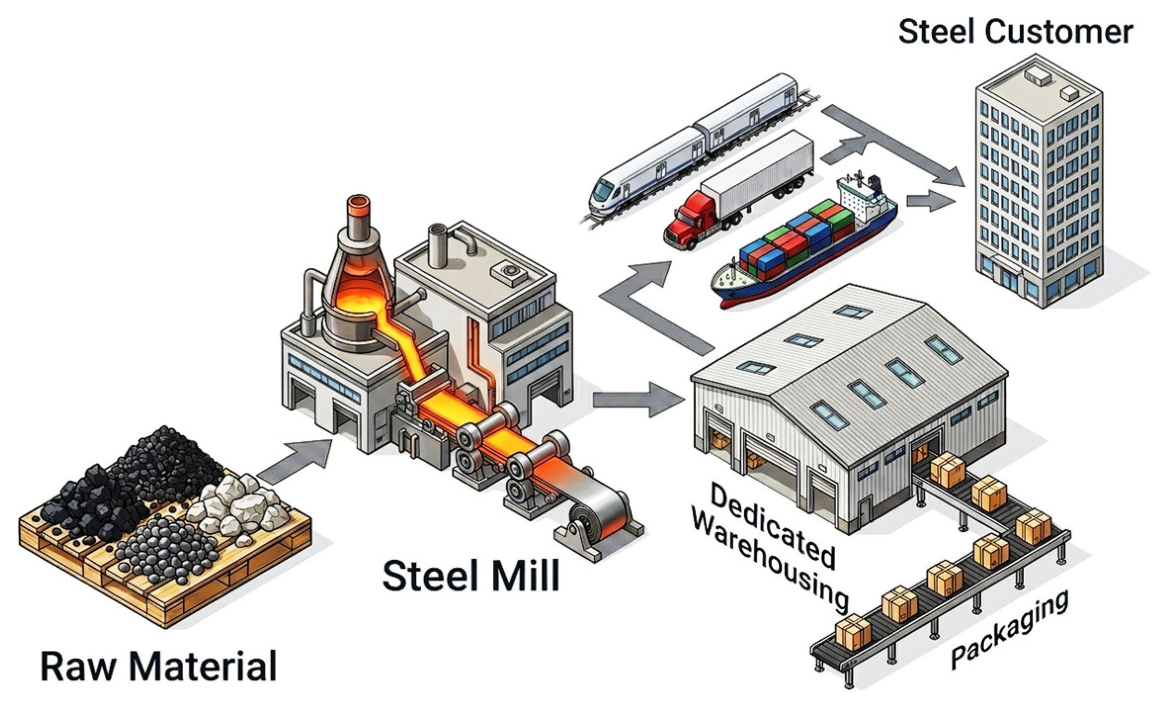
The supply chain network under consideration consists of four echelons: suppliers, steel manufacturing plants, warehouses, and customer zones, as shown in Figure 1. In the forward flow, raw materials (iron ore, pitch coke, ferro-alloys, scrap, and gypsum) are procured from multiple suppliers and shipped to steel plants. At each plant, steel products (long products: rebar and wire rod; flat products: hot-rolled coils) are produced. Finished products are then packaged (options: no packaging, wire tying, plastic packaging, VCI paper, or premium export packaging) and moved to dedicated warehouses for storage before final delivery to customers. The model also incorporates a reverse logistics loop where scrap steel is collected from customers, processed at a collection center, and returned to plants as raw material, completing the circular economy cycle. The problem involves determining optimal material flows, production quantities, inventory levels, transportation mode selection, and storage location assignments over the planning horizon. For the environmental objectives, the reduction in carbon emissions, water wastage, and energy consumption is targeted.

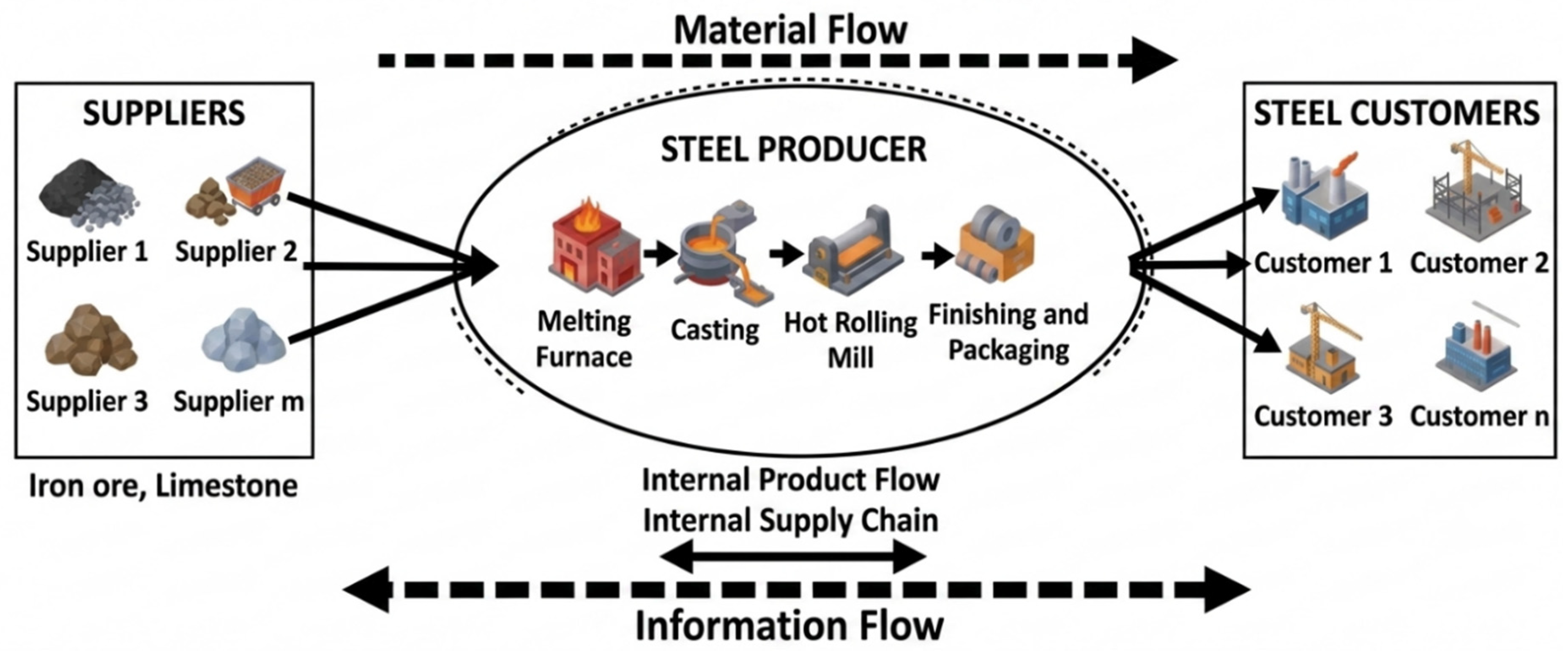
Figure 2 provides a more detailed view of the internal and external supply chain relationships. It distinguishes between material flow, internal product flow, and information flow. The figure illustrates how information and materials circulate across the network.

Three conflicting objectives are considered in this study: (1) minimizing total supply chain cost, (2) minimizing customer tardiness, and (3) minimizing environmental impact.

In order to facilitate the construction of the mathematical model, the following assumptions are made:

• Demand is deterministic and known for each month of the planning horizon.
• Production capacity at each plant is fixed and known.
• Transportation capacity for each mode is fixed per month.
• Storage capacity at each warehouse is limited.
• Each storage location can hold only one product type at a time.
• Processing times, loading times, unloading times, and travel times are deterministic.
• Backlogging is permitted; Shortage is allowed but penalized through the tardiness objective function.
• No quantity discounts are considered for raw material purchase; all unit costs are constant.
• A hybrid make-to-stock (MTS) and make-to-order (MTO) strategy is considered. Production is planned based on demand forecasts over the planning horizon, and finished goods are held in inventory (MTS). However, customer-specific packaging options and the possibility of backlogging (penalized through the tardiness objective) introduce MTO characteristics, as orders may be delayed or customized to individual customer requirements.

We acknowledge that real-world steel supply chains are characterized by considerable uncertainty in customer demand, travel times (due to traffic, port delays, or customs), and processing times (due to equipment availability or quality variations). However, this study adopts a deterministic modeling approach for the following reasons. First, the primary objective is to develop a tractable, exact multi-objective MILP framework that integrates dedicated warehousing with circular economy principles; deterministic parameters allow us to establish a baseline model and validate its structure. Second, the tactical planning horizon (monthly periods over one year) enables the use of reasonably stable forecasts, and many steel plants operate with master production schedules based on confirmed orders and safety stock policies that absorb moderate fluctuations. Third, this deterministic model serves as a foundation for future robust optimization or stochastic programming extensions, which are beyond the scope of the present work but acknowledged as a clear limitation and research direction. Therefore, while we recognize the presence of uncertainty, the current model provides a necessary first step toward more advanced methods.

The model adopts a dedicated warehousing policy, where each product-packaging combination is assigned to a fixed storage location. From a managerial perspective, this policy offers four advantages over shared or randomized storage. First, it enables batch-level traceability of returned scrap to its original source, which is essential for quality control and circular economy compliance. Second, it reduces unproductive labor hours and energy consumption by minimizing search and travel time for material handling equipment, directly lowering operational costs. Third, it simplifies inventory audits and cycle counting because storage locations are predetermined, improving inventory accuracy and reducing stock discrepancies. Fourth, it provides predictable travel paths, which enhances worker safety and enables more reliable productivity planning. While dedicated warehousing requires more storage space than shared policies, the trade-off is justified in the context of steel supply chains where traceability, cost control, and safety are managerial priorities.

4. The Mixed-Integer Linear Programming (MILP) Model

4.1. Notations

The notations used for the developed mathematical model are summarized in

Table 2. Notations used in the mathematical model.

Category	Symbol	Description
Indexes and sets	t ∈ T	set of time periods
	i ∈ I	set of products
	k ∈ K	set of packaging options
	s ∈ S	set of $\mathrm{suppliers}$
	r ∈ R	set of raw materials
	p ∈ P	set of steelmaking plants
	w ∈ W	set of warehouses
	l ∈ L	set of locations
	c ∈ C	set of customers
	m ∈ M	$\mathrm{set} \mathrm{of} \mathrm{transportation} \mathrm{modes}$ (truck, rail, ship)
	d ∈ D	set of collection centers for scrap
	q ∈ Q	set of qualities of collected scrap
	e ∈ E	set of energy sources/technologies
	a ∈ A	set of water resources
Demand and capacity parameters	${\mathrm{D}}_{\mathrm{i},\mathrm{c},\mathrm{k},\mathrm{t}}$	demand of product i of packaging k for customer $c$ in period $t$(ton)
	$Du{e}_{i,c,k,t}$	due date for product i of packaging k for customer $c$ in period $t$
	BOM	Bill of materials: amount of raw material r required per ton of product i (ton/ton)
	${\mathrm{S}\mathrm{R}\mathrm{C}}_{\mathrm{s},\mathrm{r},\mathrm{t}}$	supply capacity of suppliers for raw material r in period t (ton)
	${\mathrm{P}\mathrm{C}}_{\mathrm{i},\mathrm{p},\mathrm{t}}$	production capacity of product $i$ at plant $p$ during period $t$ (ton)
	${\mathrm{S}\mathrm{C}}_{\mathrm{i},\mathrm{w}}$	storage capacity of product $i$ at warehouse $w$(ton)
	$\mathrm{C}\mathrm{a}\mathrm{p}\mathrm{L}\mathrm{o}\mathrm{c}\mathrm{a}\mathrm{t}\mathrm{i}\mathrm{o}\mathrm{n}$	storage capacity of location l in warehousing w (ton)
	${\mathrm{S}\mathrm{C}\mathrm{R}\mathrm{C}}_{\mathrm{d},\mathrm{q},\mathrm{t}}$	collection capacity of collection center d of scrap of quality q in period t (ton)
	${\mathrm{T}\mathrm{C}}_{\mathrm{m},\mathrm{t}}$	transportation capacity of transportation mode m per trip during period t (ton)
	${\mathrm{E}\mathrm{C}\mathrm{p}}_{\mathrm{e},\mathrm{p},\mathrm{t}}$	energy usage capacity for energy source e in plant p in period t (KW·h)
	${\mathrm{E}\mathrm{C}\mathrm{w}}_{\mathrm{e},\mathrm{w},\mathrm{t}}$	energy usage capacity for energy source e in warehouse w in period t (KW·h)
	${\mathrm{W}\mathrm{C}}_{\mathrm{a},\mathrm{p},\mathrm{t}}$	water resource capacity for water resource a in plant p in period t (${\mathrm{m}}^3)$
Cost parameters	${fCs}_s$	fixed cost of selecting supplier s in period $t$ ($)
	${fCp}_p$	fixed cost of using plant p in period $t$ ($)
	${fCd}_d$	fixed cost of establishing collection center d in period $t$ ($)
	${fCw}_w$	fixed cost of operating warehouse $w$ in period $t$ ($)
	${fCm}_m$	fixed cost of utilizing transportation mode m in period $t$ ($)
	${cp}_{p,i,t}^{prod}$	unit production cost of product $i$ at plant $p$ in $period t$ ($)
	${ck}_{k,i}^{pack}$	unit packaging cost for product $i$ using packaging $k$ ($)
	${cs}_{r,s,t}^{pur}$	purchasing cost of raw material r from supplier s during period $t (\mathrm{\$}/\mathrm{t}\mathrm{o}\mathrm{n})$
	${cq}_{d,q,t}^{collect}$	collection cost of scrap of quality q in collection center d during period $t (\mathrm{\$}/\mathrm{t}\mathrm{o}\mathrm{n})$
	${\mathrm{h}}_{w,i}$	inventory holding cost per unit of product $i$ at warehouse $w$ per period $(\mathrm{\$}/\mathrm{t}\mathrm{o}\mathrm{n})$
	${csp}_{s,p,m}^{trans}$	transferring cost per unit from supplier s to plant p using mode $m$ $(\mathrm{\$}/\mathrm{t}\mathrm{o}\mathrm{n})$
	${cpw}_{p,w,m}^{trans}$	transferring cost per unit from plant p to warehouse w using mode $m$ $(\mathrm{\$}/\mathrm{t}\mathrm{o}\mathrm{n})$
	${cwc}_{w,c,m}^{trans}$	transferring cost per unit from warehouse w to customer c using mode $m$ $(\mathrm{\$}/\mathrm{t}\mathrm{o}\mathrm{n})$
	${cdq}_{d,p,m}^{trans}$	transferring cost per unit from collection center d to plant p using mode $m (\mathrm{\$}/\mathrm{t}\mathrm{o}\mathrm{n})$
	${cm}_m^{trans}$	transportation cost for transportation mode m per each trip $(\mathrm{\$}/\mathrm{t}\mathrm{r}\mathrm{i}\mathrm{p})$
	${Cp}_{e,p,t}$	unit energy cost for energy source e in plant p during period $t (\mathrm{\$}/\mathrm{K}\mathrm{W}·\mathrm{h})$
	${Cw}_{e,w,t}$	unit energy cost for energy source e in warehouse w during period $t$ ($/KW·h)
	${Ca}_{a,p,t}$	unit water cost for water resource a in plant p during period $t$ ($/${\mathrm{m}}^3$)
Time parameters	${\tau pw}_{p,w,m}$	travel time from plant $p$ to warehouse $w$ using mode $m$
	${\tau wc}_{w,c,m}$	travel time from warehouse $w$ to customer $c$ using mode $m$
	${\tau k}_{i,k}^{pack}$	packaging time per unit of product $i$ with packaging $k$
	${\tau l}_{p,w}^{load},{\tau u}_w^{unloaad}$	fixed loading/unloading times per trip
	${Pr\tau }_{i,p}$	processing time for product i in plant p (time/ton)
	$Ma{x}_{Monthly}$	maximum allowable tardiness limit for each customer c at period t
Environmental parameters	${ep}_{p,i,t}^{prod}$	energy consumption per unit of product $i$ at plant $p$ during period t (KW·h/ton)
	${ew}_{w,i,t}$	energy consumption per unit stored in warehouse $w$ during period t (kW·h/unit)
	${\mathrm{a}}_{p,i,t}$	water usage per unit of product i at plant p in period t (${\mathrm{m}}^3$/ton)
	${\alpha }_m^{{CO}_2}$	average carbon emission for mode $m (\mathrm{t}\mathrm{o}\mathrm{n}/\mathrm{t}\mathrm{r}\mathrm{i}\mathrm{p})$
	${\beta }_e^{{CO}_2}$	average carbon emissions for energy source e $(\mathrm{t}\mathrm{o}\mathrm{n}/\mathrm{K}\mathrm{W}·\mathrm{h})$
	${\delta }_a$	average ecological effect of water resource a (1/${\mathrm{m}}^3)$
	${\alpha }_m^{max}, {\alpha }_m^{min}$	max/min carbon emission of transportation mode m
	${\beta }_e^{max}, {\beta }_e^{min}$	max/min carbon emission of energy source e
	${\mathrm{\delta }}^{max}, {\mathrm{\delta }}^{min}$	max/min ecological effect of water usage
	$\tau$	Take-back policy to return scrap (%)
Additional modeling parameter	$\mathrm{M}$	large positive constant
Material flow decision variables	${\mathrm{x}}_{\mathrm{p},\mathrm{i},\mathrm{k},\mathrm{t}}$	quantity of product $\mathrm{i}$ produced at plant $\mathrm{p}$ using package k in period $\mathrm{t} \left(\mathrm{t}\mathrm{o}\mathrm{n}\right)$
	${\mathrm{Y}\mathrm{S}}_{\mathrm{r},\mathrm{s},\mathrm{p},\mathrm{m},\mathrm{t}}$	quantity of raw material r shipped from supplier s to plant p using mode m in period $t$ $\left(\mathrm{t}\mathrm{o}\mathrm{n}\right)$
	${\mathrm{Y}\mathrm{D}}_{\mathrm{q},\mathrm{d},\mathrm{p},\mathrm{m},\mathrm{t}}$	quantity of scrap with quality q shipped from collection center d to plant p using mode m in period $t \left(\mathrm{t}\mathrm{o}\mathrm{n}\right)$
	${\mathrm{Y}\mathrm{P}}_{\mathrm{p},\mathrm{w},\mathrm{i},\mathrm{k},\mathrm{m},\mathrm{t}}$	quantity of product $i$ of package k shipped from plant p to warehouse $w$ using mode m in period $t$ (ton)
	${\mathrm{Y}\mathrm{W}}_{\mathrm{w},\mathrm{c},\mathrm{i},\mathrm{k},\mathrm{m},\mathrm{t}}$	quantity of product $i$ of package k shipped from warehouse $w$ to customer $c$ using mode $m$ in period $t$ (ton)
Inventory decision variables	${\mathrm{I}}_{\mathrm{w},\mathrm{i},\mathrm{k},\mathrm{t}}$	inventoried quantity of product $i$ of package k at warehouse w at end of period (ton)
	Si,k,p,w,l,t	quantity of product i of package k is shipped from production plant p to location l in warehouse w in period t
	${\mathrm{Q}\mathrm{l}\mathrm{o}\mathrm{c}}_{\mathrm{i},\mathrm{k},\mathrm{l},\mathrm{w},\mathrm{t}}$	quantity of product i of packaging k stored in location l in warehouse w at time t
	R i,k,l,w,c,t	quantity of product i of package k is retrieved from location l in warehouse w in period t
Time and tardiness decision variables	${\mathrm{B}\mathrm{a}\mathrm{c}\mathrm{k}\mathrm{l}\mathrm{o}\mathrm{g}}_{\mathrm{i},\mathrm{k},\mathrm{c},\mathrm{t}}$	amount delayed of product i of packaging k for customer c at time t
	max_tardyc,t	maximum tardiness per customer c
	${Rel}_{\mathrm{i},\mathrm{k},\mathrm{p},\mathrm{t}}$	release time at which product $i \mathrm{o}\mathrm{f} \mathrm{p}\mathrm{a}\mathrm{c}\mathrm{k}\mathrm{a}\mathrm{g}\mathrm{i}\mathrm{n}\mathrm{g} k$ departs plant $p$ in period $t$
	${WarArr}_{\mathrm{i},\mathrm{k},\mathrm{p},\mathrm{l},\mathrm{w},\mathrm{m},\mathrm{t}}$	arrival time of product $i \mathrm{o}\mathrm{f} \mathrm{p}\mathrm{a}\mathrm{c}\mathrm{k}\mathrm{a}\mathrm{g}\mathrm{i}\mathrm{n}\mathrm{g} k$ from plant p to location l in warehouse w using mode $m at time t$
	${Arr}_{\mathrm{i},\mathrm{k},\mathrm{w},\mathrm{c},\mathrm{m},\mathrm{t}}$	arrival time of product $i \mathrm{o}\mathrm{f} \mathrm{p}\mathrm{a}\mathrm{c}\mathrm{k}\mathrm{a}\mathrm{g}\mathrm{i}\mathrm{n}\mathrm{g} k$ from warehouse w at customer $c$ using mode $m$
	${\mathrm{C}\mathrm{o}\mathrm{m}\mathrm{p}}_{\mathrm{i},\mathrm{p},\mathrm{t}}$	production completion time for product $i$ in plant $p$ in period $t$
Number of trips decision variables	${\mathrm{N}\mathrm{T}\mathrm{s}\mathrm{p}}_{\mathrm{s},\mathrm{p},\mathrm{m},\mathrm{t}}$	number of trips of transportation mode m from supplier s to plant p in period t
	${\mathrm{N}\mathrm{T}\mathrm{p}\mathrm{w}}_{\mathrm{p},\mathrm{w},\mathrm{m},\mathrm{t}}$	number of trips of transportation mode m from plant p to warehouse w in period t
	${\mathrm{N}\mathrm{T}\mathrm{d}\mathrm{p}}_{\mathrm{d},\mathrm{p},\mathrm{m},\mathrm{t}}$	number of trips of transportation mode m from collection center d to plant p in period t
	${\mathrm{N}\mathrm{T}\mathrm{w}\mathrm{c}}_{\mathrm{w},\mathrm{c},\mathrm{m},\mathrm{t}}$	number of trips of transportation mode m from warehouse w to customer c in period t
Normalized environmental decision variables	$Z_m^{{CO}_2}$	normalized value of the total carbon emission of transportation modes
	$Z_e^{{CO}_2}$	normalized value of the total carbon emission of energy consumption
	$Z^a$	normalized value of the ecological effect of water usage
Resource consumption decision variables	$W_{a,p,t}$	water usage at plant p for water resource a in period $t \left({\mathrm{m}}^3\right)$
	${Ep}_{e,p,t},{Ew}_{e,w,t}$	energy consumed at plant p/warehouse w in period $t (\mathrm{K}\mathrm{W}·\mathrm{h})$
Binary decision variables	${\mathrm{S}\mathrm{s}}_{\mathrm{s},\mathrm{t}}$	$\in \left\{\mathrm{0,1}\right\}$: 1 if supplier s is selected in period $t$
	${\mathrm{S}\mathrm{p}}_{\mathrm{p},\mathrm{t}}$	$\in \left\{\mathrm{0,1}\right\}$: 1 if plant p is equipped in period $t$
	${\mathrm{S}\mathrm{i}}_{\mathrm{i},\mathrm{p},\mathrm{t}}$	$\in \left\{\mathrm{0,1}\right\}$: 1 if product i is produced in plant p in period $t$
	${\mathrm{S}\mathrm{s}\mathrm{p}}_{1\mathrm{m},\mathrm{t}}$	$\in \left\{\mathrm{0,1}\right\}$: 1 if mode $m$ is used in period $t$ from supplier to production plant
	${\mathrm{S}\mathrm{d}\mathrm{p}}_{2\mathrm{m},\mathrm{t}}$	$\in \left\{\mathrm{0,1}\right\}$: 1 if mode $m$ is used in period $t$ from collection center to production plant
	${\mathrm{S}\mathrm{p}\mathrm{w}}_{3\mathrm{m},\mathrm{t}}$	$\in \left\{\mathrm{0,1}\right\}$: 1 if mode $m$ is used in period $t$ from production plant to warehousing
	${\mathrm{S}\mathrm{w}\mathrm{c}}_{4\mathrm{m},\mathrm{t}}$	$\in \left\{\mathrm{0,1}\right\}$: 1 if mode $m$ is used in period $t$ from warehousing to customer
	${\mathrm{S}\mathrm{d}}_{\mathrm{d},\mathrm{t}}$	$\in \left\{\mathrm{0,1}\right\}$: 1 if collection center d is established in period $t$
	${\mathrm{S}\mathrm{w}}_{\mathrm{w},\mathrm{t}}$	$\in \left\{\mathrm{0,1}\right\}$: 1 if warehouse $w$ is operated in period $t$
	${De}_{i,k,l,w}$	$\in \left\{\mathrm{0,1}\right\}$:1 if location l in warehouse $w$ is dedicated to product i of packaging k
	${\mathrm{L}\mathrm{o}\mathrm{c}}_{\mathrm{i},\mathrm{k},\mathrm{l},\mathrm{w},\mathrm{t}}$	$\in \left\{\mathrm{0,1}\right\}$: 1 if location l in warehouse w is occupied by product i of package k in period t
	${ShipD}_{i,k,l,w,c,t}$	$\in \left\{\mathrm{0,1}\right\}$: 1 if product i of package k is transported from location l in warehouse w to customer c at period t
	Ziklwcmt	$\in \left\{\mathrm{0,1}\right\}$: used for linearization
	Y	auxiliary binary variable used for linearization of nonlinear constraints

. They are categorized according to their types (parameters or decision variables) and according to their usage in the model.

Considering the notations of this paper, the proposed model is introduced in the following subsections. First, the objective functions of the model are presented, and then the model constraints are explained.

4.2. Objective Functions

The objective functions of the suggested model are minimizing total expected cost, minimizing the environmental effects, and minimizing expected tardiness.

The total expected costs can be divided into four sections: total fixed cost for selection or establishment, total transportation costs, total energy and water resources costs, and total production or procurement costs. The first objective of the total cost of the system is illustrated in Equation (1)

$$\min TC=c_1+c_2+c_3+c_4$$

(1)

Equation (2) represents the five fixed costs of selecting supplier s, utilizing steel plant p, establishing collection center d, operating warehouse w, and using transportation mode m, respectively.

$$\begin{gathered} c_1={\sum }_{s,t}{fCs}_s · {\mathrm{S}\mathrm{s}}_{s,t}+{\sum }_{p,t}{fCp}_p · {\mathrm{S}\mathrm{p}}_{p,t}+{\sum }_{d,t}{fCd}_d · {\mathrm{S}\mathrm{d}}_{d,t}+{\sum }_{w,t}{fCw}_w· {\mathrm{S}\mathrm{w}}_{\mathrm{w},\mathrm{t}}+ \\ {\sum }_{m,t}{fCm}_m · {(\mathrm{S}\mathrm{s}\mathrm{p}}_{1m,t}+{\mathrm{S}\mathrm{d}\mathrm{p}}_{2\mathrm{m},\mathrm{t}}+{\mathrm{S}\mathrm{p}\mathrm{w}}_{3\mathrm{m},\mathrm{t}}+{\mathrm{S}\mathrm{w}\mathrm{c}}_{4\mathrm{m},\mathrm{t}}) \end{gathered}$$

(2)

Equation (3) considers transportation cost of raw material r from supplier s to steel plant p using transportation mode m, transportation cost of scrap of quality q from collection center d to steel plant p using transportation mode m, transportation cost of product i from steel plant p to warehouse w using transportation mode m, transportation cost of product i from warehouse w to customer c using transportation mode m, and costs based on the number of trips respectively.

$$\begin{array}{c}{c}_2={\sum }_{s,p,m,r,t}{csp}_{s,p,m}^{trans}· {\mathrm{Y}\mathrm{S}}_{\mathrm{r},\mathrm{s},\mathrm{p},\mathrm{m},\mathrm{t}}+{\sum }_{d,p,m,q,t}{cdq}_{d,p,m}^{trans} · {\mathrm{Y}\mathrm{D}}_{\mathrm{q},\mathrm{d},\mathrm{p},\mathrm{m},\mathrm{t}}+{\sum }_{p,w,m,i,k,t}{cpw}_{p,w,m}^{trans} ·{\mathrm{Y}\mathrm{P}}_{\mathrm{p},\mathrm{w},\mathrm{i},\mathrm{k},\mathrm{m},\mathrm{t}}+\hfill \\ {\sum }_{w,c,m,i,k,t}{cwc}_{w,c,m}^{trans}· {\mathrm{Y}\mathrm{W}}_{\mathrm{w},\mathrm{c},\mathrm{i},\mathrm{k},\mathrm{m},\mathrm{t}}+{\sum }_m{cm}_m^{trans}({\sum }_{s,p,t}{\mathrm{N}\mathrm{T}\mathrm{s}\mathrm{p}}_{\mathrm{s},\mathrm{p},\mathrm{m},\mathrm{t}}+{\sum }_{p,w,t}{\mathrm{N}\mathrm{T}\mathrm{p}\mathrm{w}}_{\mathrm{p},\mathrm{w},\mathrm{m},\mathrm{t}}+{\sum }_{d,p,t}{\mathrm{N}\mathrm{T}\mathrm{d}\mathrm{p}}_{\mathrm{d},\mathrm{p},\mathrm{m},\mathrm{t}}+\hfill \\ {\sum }_{w,c,t}{\mathrm{N}\mathrm{T}\mathrm{w}\mathrm{c}}_{\mathrm{w},\mathrm{c},\mathrm{m},\mathrm{t}})\hfill \end{array}$$

(3)

Equation (4) represents the energy and water usage cost in production plant p and warehouse w.

$$c_3={\sum }_{e,p,t}{Cp}_{e,p,t} · {Ep}_{e,p,t}+{\sum }_{e,w,t}{Cw}_{e,w,t} · {Ew}_{e,w,t}+{\sum }_{a,p,t}{Ca}_{a,p,t}· W_{a,p,t}$$

(4)

Equation (5) represents other costs of production, packaging, raw material purchasing, and collection.

$$\begin{gathered} c_4={\sum }_{p,i,k,t}{(cp}_{p,i,t}^{prod}+{ck}_{k,i}^{pack})·{\mathrm{x}}_{\mathrm{p},\mathrm{i},\mathrm{k},\mathrm{t}}+{\sum }_{s,r,p,m,t}{cs}_{r,s,t}^{pur}·{\mathrm{Y}\mathrm{S}}_{\mathrm{r},\mathrm{s},\mathrm{p},\mathrm{m},\mathrm{t}}+{\sum }_{p,d,q,m,t}{cq}_{d,q,t}^{collect}·{\mathrm{Y}\mathrm{D}}_{\mathrm{q},\mathrm{d},\mathrm{p},\mathrm{m},\mathrm{t}}+ \\ {\sum }_{w,i,k,t}{\mathrm{h}}_{w,i} ·{\mathrm{I}}_{\mathrm{w},\mathrm{i},\mathrm{k},\mathrm{t}} \end{gathered}$$

(5)

The second objective is to minimize the normalized environmental impact from transportation emissions, energy-related emissions, and water ecological effects, as illustrated in Equation (6). To combine the three environmental components into a single objective function, each component is normalized using the min–max method. This allows all components to be aggregated into a single environmental objective when objectives have different units and magnitudes.

$$min EE = Z_m^{{CO}_2}+Z_e^{{CO}_2}+Z^a$$

(6)

The first term represents the normalized value of the total carbon emissions of the transportation modes and is calculated based on average carbon emission of transportation mode m and number of trips it made as illustrated in Equation (7) while Equation (8) is the normalized value of carbon emission of each energy source in production plants and warehousing and the corresponding amount of used energy and Equation (9) is the normalized ecological effect of water determined by the amount of source a and its effect.

$$Z_m^{{CO}_2} ={\displaystyle \frac{\left({\alpha }_m^{{CO}_2}\left[{\sum }_{s,p,t}{\mathrm{N}\mathrm{T}\mathrm{s}\mathrm{p}}_{\mathrm{s},\mathrm{p},\mathrm{m},\mathrm{t}}+{\sum }_{d,p,t}{\mathrm{N}\mathrm{T}\mathrm{d}\mathrm{p}}_{\mathrm{d},\mathrm{p},\mathrm{m},\mathrm{t}}+{\sum }_{p,w,t}{\mathrm{N}\mathrm{T}\mathrm{p}\mathrm{w}}_{\mathrm{p},\mathrm{w},\mathrm{m},\mathrm{t}}+{\sum }_{w,c,t}{\mathrm{N}\mathrm{T}\mathrm{w}\mathrm{c}}_{\mathrm{w},\mathrm{c},\mathrm{m},\mathrm{t}}\right]\right)-{\alpha }_m^{min}}{{\alpha }_m^{max}-{\alpha }_m^{min}}}$$

(7)

$$Z_e^{{CO}_2} ={\displaystyle \frac{\left({\beta }_e^{{CO}_2} · {\sum }_{p,t} {Ep}_{e,p,t}+{\sum }_{w,t}{Ew}_{e,w,t})\right)-{\beta }_e^{min}}{{\beta }_e^{max}-{\beta }_e^{min}}}$$

(8)

$$Z^a ={\displaystyle \frac{\left({\delta }_a · {\sum }_{p,t}{W}_{a,p,t})\right)-{\delta }^{min}}{{\delta }^{max}-{\delta }^{min}}}$$

(9)

The third objective function is minimizing the expected tardiness as shown in Equation (10).

$$\mathrm{m}\mathrm{i}\mathrm{n} TD = \sum _{c,t}{max\text{\_}\mathrm{t}\mathrm{a}\mathrm{r}\mathrm{d}\mathrm{y}}_{c,t}$$

(10)

4.3. Constraints

4.3.1. Material Flow Constraints:

Equations (11) and (12) ensure global demand fulfillment and ensure that all production is shipped through warehouses before reaching customers. Equation (13) links production quantities to plant activation status. Demand satisfaction with backlog is ensured by Equations (14) and (15). Raw material requirements, including scrap recycling, are determined by Equation (16), while Equation (17) maintains inventory balance at each warehouse.

$$\sum _{\mathrm{p},\mathrm{t}}{\mathrm{x}}_{\mathrm{p},\mathrm{i},\mathrm{k},\mathrm{t}} \ge \sum _{\mathrm{c},\mathrm{t}}{\mathrm{D}}_{\mathrm{i},\mathrm{c},\mathrm{k},\mathrm{t}}\hspace{1em}\hspace{1em}\forall \mathrm{i},\mathrm{k}$$

(11)

$${\mathrm{x}}_{\mathrm{p},\mathrm{i},\mathrm{k},\mathrm{t}}=\sum _{\mathrm{w},\mathrm{m}}{\mathrm{Y}\mathrm{P}}_{\mathrm{p},\mathrm{w},\mathrm{i},\mathrm{k},\mathrm{m},\mathrm{t}}\hspace{1em}\hspace{1em}\forall \mathrm{i},\mathrm{k},\mathrm{p},\mathrm{t}$$

(12)

$$\begin{gathered} \sum _{\mathrm{k}}{\mathrm{x}}_{\mathrm{p},\mathrm{i},\mathrm{k},\mathrm{t}} \le \mathrm{M}· {\mathrm{S}\mathrm{i}}_{\mathrm{i},\mathrm{p},\mathrm{t}}\hspace{1em}\hspace{1em}\forall \mathrm{i},\mathrm{p},\mathrm{t} \\ \sum _{\mathrm{k}}{\mathrm{x}}_{\mathrm{p},\mathrm{i},\mathrm{k},\mathrm{t}} \ge {\mathrm{S}\mathrm{i}}_{\mathrm{i},\mathrm{p},\mathrm{t}} \end{gathered}$$

(13)

$$\sum _{\mathrm{w},\mathrm{m}}{\mathrm{Y}\mathrm{W}}_{\mathrm{w},\mathrm{c},\mathrm{i},\mathrm{k},\mathrm{m},\mathrm{t}} \le {\mathrm{D}}_{\mathrm{i},\mathrm{c},\mathrm{k},\mathrm{t}}\hspace{1em}\hspace{1em}\forall \mathrm{i},\mathrm{k},\mathrm{c},\mathrm{t}$$

(14)

$$\sum _{\mathrm{w},\mathrm{m},\mathrm{t}}{\mathrm{Y}\mathrm{W}}_{\mathrm{w},\mathrm{c},\mathrm{i},\mathrm{k},\mathrm{m},\mathrm{t}} = \sum _{\mathrm{t}}{\mathrm{D}}_{\mathrm{i},\mathrm{c},\mathrm{k},\mathrm{t}}\hspace{1em}\hspace{1em}\forall \mathrm{i},\mathrm{k},\mathrm{c}$$

(15)

$$\sum _{\mathrm{s},\mathrm{m}}{\mathrm{Y}\mathrm{S}}_{\mathrm{r},\mathrm{s},\mathrm{p},\mathrm{m},\mathrm{t}} +\sum _{\mathrm{q},\mathrm{d},\mathrm{m}}{\mathrm{Y}\mathrm{D}}_{\mathrm{q},\mathrm{d},\mathrm{p},\mathrm{m},\mathrm{t}-1}\ge \sum _{\mathrm{i},\mathrm{k}}{{\mathrm{B}\mathrm{O}\mathrm{M}}_{\mathrm{r},\mathrm{i}}·\mathrm{x}}_{\mathrm{p},\mathrm{i},\mathrm{k},\mathrm{t}}\hspace{1em}\hspace{1em}\forall \mathrm{r},\mathrm{p},\mathrm{t}|{\mathrm{Y}\mathrm{D}}_{\mathrm{q},\mathrm{d},\mathrm{p},\mathrm{m},\mathrm{t}}=0 \mathrm{a}\mathrm{t} \mathrm{t}=1$$

(16)

$${\mathrm{I}}_{\mathrm{w},\mathrm{i},\mathrm{k},\mathrm{t}}={\mathrm{I}}_{\mathrm{w},\mathrm{i},\mathrm{k},\mathrm{t}-1}+\sum _{\mathrm{p},\mathrm{m}}{\mathrm{Y}\mathrm{P}}_{\mathrm{p},\mathrm{w},\mathrm{i},\mathrm{k},\mathrm{m},\mathrm{t}}-\sum _{\mathrm{c},\mathrm{m}}{\mathrm{Y}\mathrm{W}}_{\mathrm{w},\mathrm{c},\mathrm{i},\mathrm{k},\mathrm{m},\mathrm{t}}\hspace{1em}\hspace{1em}\forall \mathrm{w},\mathrm{i},\mathrm{k},\mathrm{t}|{\mathrm{I}}_{\mathrm{w},\mathrm{i},\mathrm{k},\mathrm{t}}=0 \mathrm{a}\mathrm{t} \mathrm{t}=1$$

(17)

4.3.2. Capacity Constraints

Equation (18) ensures the capacity constraint of suppliers. Equation (19) encompasses the production capacity. Equations (20) and (21) illustrate the warehousing and collection centers’ capacity. Equations (22)–(25) determine the required number of trips for each transportation mode between every two nodes. Equations (26)–(29) define the capacity constraints for transportation modes between every two nodes.

$$\sum _{\mathrm{p},\mathrm{m}}{\mathrm{Y}\mathrm{S}}_{\mathrm{r},\mathrm{s},\mathrm{p},\mathrm{m},\mathrm{t}} \le {\mathrm{S}\mathrm{s}}_{\mathrm{s},\mathrm{t}}·{\mathrm{S}\mathrm{R}\mathrm{C}}_{\mathrm{s},\mathrm{r},\mathrm{t}}\hspace{1em}\hspace{1em}\forall \mathrm{s},\mathrm{r},\mathrm{t}$$

(18)

$$\sum _{\mathrm{k}}{\mathrm{x}}_{\mathrm{p},\mathrm{i},\mathrm{k},\mathrm{t}}\le {\mathrm{S}\mathrm{p}}_{\mathrm{p},\mathrm{t}}·{\mathrm{P}\mathrm{C}}_{\mathrm{i},\mathrm{p},\mathrm{t}}\hspace{1em}\hspace{1em}\forall \mathrm{p},\mathrm{i},\mathrm{t}$$

(19)

$$\sum _{\mathrm{k}}{\mathrm{I}}_{\mathrm{w},\mathrm{i},\mathrm{k},\mathrm{t}} \le {\mathrm{S}\mathrm{w}}_{\mathrm{w},\mathrm{t}}·{\mathrm{S}\mathrm{C}}_{\mathrm{i},\mathrm{w}}\hspace{1em}\hspace{1em}\forall \mathrm{i},\mathrm{w},\mathrm{t}$$

(20)

$$\sum _{\mathrm{p},\mathrm{m}}{\mathrm{Y}\mathrm{D}}_{\mathrm{q},\mathrm{d},\mathrm{p},\mathrm{m},\mathrm{t}} \le {\mathrm{S}\mathrm{d}}_{\mathrm{d},\mathrm{t}}· {\mathrm{S}\mathrm{C}\mathrm{R}\mathrm{C}}_{\mathrm{d},\mathrm{q},\mathrm{t}}\hspace{1em}\hspace{1em}\forall \mathrm{d},\mathrm{q},\mathrm{t}$$

(21)

$$\sum _{\mathrm{r}}{\mathrm{Y}\mathrm{S}}_{\mathrm{r},\mathrm{s},\mathrm{p},\mathrm{m},\mathrm{t}} \le {\mathrm{T}\mathrm{C}}_{\mathrm{m},\mathrm{t}} · {\mathrm{N}\mathrm{T}\mathrm{s}\mathrm{p}}_{\mathrm{s},\mathrm{p},\mathrm{m},\mathrm{t}}\hspace{1em}\hspace{1em}\forall \mathrm{s},\mathrm{p},\mathrm{m},\mathrm{t}$$

(22)

$$\sum _{\mathrm{i},\mathrm{k}}{\mathrm{Y}\mathrm{P}}_{\mathrm{p},\mathrm{w},\mathrm{i},\mathrm{k},\mathrm{m},\mathrm{t}} \le {\mathrm{T}\mathrm{C}}_{\mathrm{m},\mathrm{t}} · {\mathrm{N}\mathrm{T}\mathrm{p}\mathrm{w}}_{\mathrm{p},\mathrm{w},\mathrm{m},\mathrm{t}}\hspace{1em}\hspace{1em}\forall \mathrm{p},\mathrm{w},\mathrm{m},\mathrm{t}$$

(23)

$$\sum _{\mathrm{q}}{\mathrm{Y}\mathrm{D}}_{\mathrm{q},\mathrm{d},\mathrm{p},\mathrm{m},\mathrm{t}} \le {\mathrm{T}\mathrm{C}}_{\mathrm{m},\mathrm{t}} · {\mathrm{N}\mathrm{T}\mathrm{d}\mathrm{p}}_{\mathrm{d},\mathrm{p},\mathrm{m},\mathrm{t}}\hspace{1em}\hspace{1em}\forall \mathrm{d},\mathrm{p},\mathrm{m},\mathrm{t}$$

(24)

$$\sum _{\mathrm{i},\mathrm{k}}{\mathrm{Y}\mathrm{W}}_{\mathrm{w},\mathrm{c},\mathrm{i},\mathrm{k},\mathrm{m},\mathrm{t}} \le {\mathrm{T}\mathrm{C}}_{\mathrm{m},\mathrm{t}} · {\mathrm{N}\mathrm{T}\mathrm{w}\mathrm{c}}_{\mathrm{w},\mathrm{c},\mathrm{m},\mathrm{t}}\forall \mathrm{w},\mathrm{c},\mathrm{m},\mathrm{t}$$

(25)

$$\mathrm{M}·{\mathrm{S}\mathrm{s}\mathrm{p}}_{1\mathrm{m},\mathrm{t}}\ge \sum _{\mathrm{r},\mathrm{s},\mathrm{p}}{\mathrm{Y}\mathrm{S}}_{\mathrm{r},\mathrm{s},\mathrm{p},\mathrm{m},\mathrm{t}}\hspace{1em}\hspace{1em}\forall \mathrm{m},\mathrm{t}$$

(26)

$$\mathrm{M}·{\mathrm{S}\mathrm{d}\mathrm{p}}_{2\mathrm{m},\mathrm{t}}\ge \sum _{\mathrm{d},\mathrm{q},\mathrm{p}}{\mathrm{Y}\mathrm{D}}_{\mathrm{q},\mathrm{d},\mathrm{p},\mathrm{m},\mathrm{t}}\hspace{1em}\hspace{1em}\forall \mathrm{m},\mathrm{t}$$

(27)

$$\mathrm{M}·{\mathrm{S}\mathrm{p}\mathrm{w}}_{3\mathrm{m},\mathrm{t}}\ge \sum _{\mathrm{p},\mathrm{w},\mathrm{i},\mathrm{k}}{\mathrm{Y}\mathrm{P}}_{\mathrm{p},\mathrm{w},\mathrm{i},\mathrm{k},\mathrm{m},\mathrm{t}}\hspace{1em}\hspace{1em}\forall \mathrm{m},\mathrm{t}$$

(28)

$$\mathrm{M}·{\mathrm{S}\mathrm{w}\mathrm{c}}_{4\mathrm{m},\mathrm{t}}\ge \sum _{\mathrm{w},\mathrm{c},\mathrm{i},\mathrm{k}}{\mathrm{Y}\mathrm{W}}_{\mathrm{w},\mathrm{c},\mathrm{i},\mathrm{k},\mathrm{m},\mathrm{t}}\hspace{1em}\hspace{1em}\forall \mathrm{m},\mathrm{t}$$

(29)

4.3.3. Dedicated Warehousing Constraints

Equations (30) and (31) control location assignment: each storage location holds at most one product type, each product has at least one dedicated location, and only one product type can occupy a location at any time. Equation (32) limits incoming flows to available dedicated storage capacity. Equation (33) restricts storage to pre-assigned locations only. Equation (34) ensures retrieved quantities do not exceed stored inventory. Equation (35) balances demand fulfillment with backlogging across all locations. Equation (36) distributes incoming shipments across storage locations. Equation (37) links positive shipments to binary shipping decisions. Equation (38) enforces per-location storage capacity. Equation (39) allows retrieval only from locations where products are stored. Equation (40) ensures storage occurs only in dedicated locations within capacity limits. Finally, Equation (41) guarantees that customer shipments are sourced entirely from retrieved quantities across storage locations.

$$\begin{gathered} \sum _{\mathrm{i},\mathrm{k}}{\mathrm{D}\mathrm{e}}_{\mathrm{i},\mathrm{k},\mathrm{l},\mathrm{w}}\le 1\hspace{1em}\hspace{1em}\forall \mathrm{l},\mathrm{w} \\ \sum _{\mathrm{l},\mathrm{w}}{\mathrm{D}\mathrm{e}}_{\mathrm{i},\mathrm{k},\mathrm{l},\mathrm{w}}\ge 1\hspace{1em}\hspace{1em}\forall \mathrm{i},\mathrm{k} \end{gathered}$$

(30)

$$\sum _{\mathrm{i},\mathrm{k}}{\mathrm{L}\mathrm{o}\mathrm{c}}_{\mathrm{i},\mathrm{k},\mathrm{l},\mathrm{w},\mathrm{t}}\le 1\hspace{1em}\hspace{1em}\forall \mathrm{l},\mathrm{w},\mathrm{t}$$

(31)

$$\sum _{\mathrm{p},\mathrm{m}}{\mathrm{Y}\mathrm{P}}_{\mathrm{p},\mathrm{w},\mathrm{i},\mathrm{k},\mathrm{m},\mathrm{t}}\le \sum _{\mathrm{l}}{\mathrm{D}\mathrm{e}}_{\mathrm{i},\mathrm{k},\mathrm{l},\mathrm{w}} · \mathrm{C}\mathrm{a}\mathrm{p}\mathrm{L}\mathrm{o}\mathrm{c}\mathrm{a}\mathrm{t}\mathrm{i}\mathrm{o}\mathrm{n}\hspace{1em}\hspace{1em}\forall \mathrm{i},\mathrm{k},\mathrm{w},\mathrm{t}$$

(32)

$${\mathrm{L}\mathrm{o}\mathrm{c}}_{\mathrm{i},\mathrm{k},\mathrm{l},\mathrm{w},\mathrm{t}}\le {\mathrm{D}\mathrm{e}}_{\mathrm{i},\mathrm{k},\mathrm{l},\mathrm{w}}\hspace{1em}\hspace{1em}\forall \mathrm{i},\mathrm{k},\mathrm{l},\mathrm{w},\mathrm{t}$$

(33)

$$\sum _{\mathrm{c},\mathrm{m}}{\mathrm{Y}\mathrm{W}}_{\mathrm{w},\mathrm{c},\mathrm{i},\mathrm{k},\mathrm{m},\mathrm{t}}\le \sum _{\mathrm{l}}{\mathrm{Q}\mathrm{l}\mathrm{o}\mathrm{c}}_{\mathrm{i},\mathrm{k},\mathrm{l},\mathrm{w},\mathrm{t}}\hspace{1em}\hspace{1em}\forall \mathrm{i},\mathrm{k},\mathrm{w},\mathrm{t}$$

(34)

$$\sum _{\mathrm{w},\mathrm{m}}{\mathrm{Y}\mathrm{W}}_{\mathrm{w},\mathrm{c},\mathrm{i},\mathrm{k},\mathrm{m},\mathrm{t}}+{\mathrm{B}\mathrm{a}\mathrm{c}\mathrm{k}\mathrm{l}\mathrm{o}\mathrm{g}}_{\mathrm{i},\mathrm{k},\mathrm{c},\mathrm{t}-1}={\mathrm{D}}_{\mathrm{i},\mathrm{c},\mathrm{k},\mathrm{t}}\hspace{1em}\hspace{1em}\forall \mathrm{i},\mathrm{k},\mathrm{c},\mathrm{t}|{\mathrm{B}\mathrm{a}\mathrm{c}\mathrm{k}\mathrm{l}\mathrm{o}\mathrm{g}}_{\mathrm{i},\mathrm{k},\mathrm{c},\mathrm{t}=1}=0$$

(35)

$$\sum _{\mathrm{p},\mathrm{m}}{\mathrm{Y}\mathrm{P}}_{\mathrm{p},\mathrm{w},\mathrm{i},\mathrm{k},\mathrm{m},\mathrm{t}}=\sum _{\mathrm{p},\mathrm{l}}{\mathrm{S}}_{\mathrm{i},\mathrm{k},\mathrm{p},\mathrm{w},\mathrm{l},\mathrm{t}}\hspace{1em}\hspace{1em}\forall \mathrm{i},\mathrm{k},\mathrm{w},\mathrm{t}$$

(36)

$$\begin{gathered} {\mathrm{R}}_{\mathrm{i},\mathrm{k},\mathrm{l},\mathrm{w},\mathrm{c},\mathrm{t}}\le \mathrm{M}·{\mathrm{S}\mathrm{h}\mathrm{i}\mathrm{p}\mathrm{D}}_{\mathrm{i},\mathrm{k},\mathrm{l},\mathrm{w},\mathrm{c},\mathrm{t}}\hspace{1em}\hspace{1em}\forall \mathrm{i},\mathrm{k},\mathrm{l},\mathrm{w},\mathrm{c},\mathrm{m},\mathrm{t} \\ {\mathrm{R}}_{\mathrm{i},\mathrm{k},\mathrm{l},\mathrm{w},\mathrm{c},\mathrm{t}}\ge {\mathrm{S}\mathrm{h}\mathrm{i}\mathrm{p}\mathrm{D}}_{\mathrm{i},\mathrm{k},\mathrm{l},\mathrm{w},\mathrm{c},\mathrm{t}}\hspace{1em}\hspace{1em}\forall \mathrm{i},\mathrm{k},\mathrm{l},\mathrm{w},\mathrm{c},\mathrm{m},\mathrm{t} \end{gathered}$$

(37)

$${\mathrm{D}\mathrm{e}}_{\mathrm{i},\mathrm{k},\mathrm{l},\mathrm{w}} · \mathrm{C}\mathrm{a}\mathrm{p}\mathrm{L}\mathrm{o}\mathrm{c}\mathrm{a}\mathrm{t}\mathrm{i}\mathrm{o}\mathrm{n}\ge {\mathrm{Q}\mathrm{l}\mathrm{o}\mathrm{c}}_{\mathrm{i},\mathrm{k},\mathrm{l},\mathrm{w},\mathrm{t}}\hspace{1em}\hspace{1em}\forall \mathrm{i},\mathrm{k},\mathrm{l},\mathrm{w},\mathrm{t}$$

(38)

$${\mathrm{R}}_{\mathrm{i},\mathrm{k},\mathrm{l},\mathrm{w},\mathrm{c},\mathrm{t}}\le {\mathrm{L}\mathrm{o}\mathrm{c}}_{\mathrm{i},\mathrm{k},\mathrm{l},\mathrm{w},\mathrm{t}}·\mathrm{C}\mathrm{a}\mathrm{p}\mathrm{L}\mathrm{o}\mathrm{c}\mathrm{a}\mathrm{t}\mathrm{i}\mathrm{o}\mathrm{n}\hspace{1em}\hspace{1em}\forall \mathrm{i},\mathrm{k},\mathrm{l},\mathrm{w},\mathrm{c},\mathrm{t}$$

(39)

$$\sum _{\mathrm{p}}{\mathrm{S}}_{\mathrm{i},\mathrm{k},\mathrm{p},\mathrm{w},\mathrm{l},\mathrm{t}}\le \mathrm{m}\mathrm{i}\mathrm{n}({\mathrm{D}\mathrm{e}}_{\mathrm{i},\mathrm{k},\mathrm{l},\mathrm{w}} · \mathrm{C}\mathrm{a}\mathrm{p}\mathrm{L}\mathrm{o}\mathrm{c}\mathrm{a}\mathrm{t}\mathrm{i}\mathrm{o}\mathrm{n},\mathrm{C}\mathrm{a}\mathrm{p}\mathrm{L}\mathrm{o}\mathrm{c}\mathrm{a}\mathrm{t}\mathrm{i}\mathrm{o}\mathrm{n}-{\mathrm{Q}\mathrm{l}\mathrm{o}\mathrm{c}}_{\mathrm{i},\mathrm{k},\mathrm{l},\mathrm{w},\mathrm{t}-1})\hspace{1em}\hspace{1em}\forall \mathrm{l},\mathrm{w},\mathrm{i},\mathrm{k},\mathrm{t}$$

(40)

$${\mathrm{Y}\mathrm{W}}_{\mathrm{w},\mathrm{c},\mathrm{i},\mathrm{k},\mathrm{m},\mathrm{t}}=\sum _{\mathrm{l}}{\mathrm{R}}_{\mathrm{i},\mathrm{k},\mathrm{l},\mathrm{w},\mathrm{c},\mathrm{t}}\hspace{1em}\hspace{1em}\forall \mathrm{i},\mathrm{k},\mathrm{w},\mathrm{c},\mathrm{m},\mathrm{t}$$

(41)

4.3.4. Energy and Environmental Impact Constraints

Equations (42) and (43) constrain the availability of energy sources in plants, packaging, and warehousing, while Equation (44) constrains the water usage in steel plants. Equations (45)–(47) calculate energy consumption and water usage within the steel plants and warehousing.

$${Ep}_{e,p,t}\le {\mathrm{E}\mathrm{C}\mathrm{p}}_{\mathrm{e},\mathrm{p},\mathrm{t}}\hspace{1em}\hspace{1em}\forall p,e,t$$

(42)

$${Ew}_{e,w,t}\le {\mathrm{E}\mathrm{C}\mathrm{w}}_{\mathrm{e},\mathrm{w},\mathrm{t}}\hspace{1em}\hspace{1em}\forall w,e,t$$

(43)

$${Wa}_{a,p,t}\le {\mathrm{W}\mathrm{C}}_{\mathrm{a},\mathrm{p},\mathrm{t}}\hspace{1em}\hspace{1em}\forall p,a,t$$

(44)

$$\sum _e{Ep}_{e,p,t}=\sum _{i,k}{\mathrm{x}}_{\mathrm{p},\mathrm{i},\mathrm{k},\mathrm{t}}·{ep}_{p,i,t}^{prod}\hspace{1em}\hspace{1em}\forall p,t$$

(45)

$$\sum _e{Ew}_{e,w,t}=\sum _{i,k}({\mathrm{I}}_{\mathrm{w},\mathrm{i},\mathrm{k},\mathrm{t}}+\sum _{p,m}{\mathrm{Y}\mathrm{P}}_{\mathrm{p},\mathrm{w},\mathrm{i},\mathrm{k},\mathrm{m},\mathrm{t}})·{ew}_{w,i,t}\hspace{1em}\hspace{1em}\forall w,t$$

(46)

$$\sum _a{W}_{a,p,t}=\sum _{i,k}{\mathrm{x}}_{\mathrm{p},\mathrm{i},\mathrm{k},\mathrm{t}}·{\mathrm{a}}_{p,i,t}\hspace{1em}\hspace{1em}\forall p,t$$

(47)

4.3.5. Tardiness Constraints

Equation (48) is used for linearization. Equation (49) estimates the completion time in the production stage, while Equation (50) is the release time after the production and packaging stages. Equation (51) is the arrival time to warehousing; then, Equation (52) estimates the maximum tardiness time per customer, ensuring it does not exceed a predefined limit. In steel industry practice, late delivery penalties depend on delay duration rather than backlog quantity. Minimizing maximum tardiness for each customer over a period captures this logic, ensures equitable service among customers, and prevents any single customer from experiencing excessive delay. Equation (53) ensures the amounts of scrap are satisfying the take-back policy, requiring that scrap must be utilized in the production process at a specific proportion of the steel production.

$$\begin{gathered} Z_{iklwcmt}\le {ShipD}_{i,k,l,w,c,t}\hspace{1em}\hspace{1em}\forall i,k,l,w,c,m,t \\ { Z}_{iklwcmt}\le {\mathrm{S}\mathrm{w}\mathrm{c}}_{4\mathrm{m},\mathrm{t}}\hspace{1em}\hspace{1em}\forall i,k,l,w,c,m,t \\ {Z}_{iklwcmt}\ge {ShipD}_{i,k,l,w,c,t}+{\mathrm{S}\mathrm{w}\mathrm{c}}_{4\mathrm{m},\mathrm{t}}-1\hspace{1em}\hspace{1em}\forall i,k,l,w,c,m,t \end{gathered}$$

(48)

$${\mathrm{C}\mathrm{o}\mathrm{m}\mathrm{p}}_{\mathrm{i},\mathrm{p},\mathrm{t}}\ge {\mathrm{P}\mathrm{r}\tau }_{i,p} · \sum _k{\mathrm{x}}_{\mathrm{p},\mathrm{i},\mathrm{k},\mathrm{t}}\hspace{1em}\hspace{1em}\forall i,p,t$$

(49)

$${Rel}_{\mathrm{i},\mathrm{k},\mathrm{p},\mathrm{t}} \ge {\mathrm{C}\mathrm{o}\mathrm{m}\mathrm{p}}_{\mathrm{i},\mathrm{p},\mathrm{t}}+{\tau k}_{i,k}^{pack} · {\mathrm{x}}_{\mathrm{p},\mathrm{i},\mathrm{k},\mathrm{t}} \forall \mathrm{i},\mathrm{k},\mathrm{p},\mathrm{t}$$

(50)

$$\begin{gathered} {WarArr}_{i,k,p,l,w,m,t}\ge {Rel}_{i,k,p,t}+{\tau pw}_{p,w,m}· {\mathrm{S}\mathrm{p}\mathrm{w}}_{3\mathrm{m},\mathrm{t}}+{\tau l}_{p,w}^{load} \forall i,k,p,l,w,m,t \\ {Arr}_{i,k,w,c,m,t} \ge {WarArr}_{i,k,p,l,w,m,t}+{\tau wc}_{w,c,m}· {\mathrm{S}\mathrm{w}\mathrm{c}}_{4\mathrm{m},\mathrm{t}} +{\tau u}_w^{unloaad} \\ -\mathrm{M} \left(1-{ShipD}_{i,k,l,w,c,t}\right) \forall i,k,p,l,w,c,m,t \end{gathered}$$

(51)

$$\begin{gathered} {Arr}_{i,k,w,c,m,t} - Du{e}_{i,c,k,t}\le {max\text{\_}\mathrm{t}\mathrm{a}\mathrm{r}\mathrm{d}\mathrm{y}}_{c,t} \forall i,k,w,c,m,t \\ {max\text{\_}\mathrm{t}\mathrm{a}\mathrm{r}\mathrm{d}\mathrm{y}}_{c,t} \le Ma{x}_{Monthly} \forall c,t \end{gathered}$$

(52)

$$\sum _{d,q,m}{\mathrm{Y}\mathrm{D}}_{\mathrm{q},\mathrm{d},\mathrm{p},\mathrm{m},\mathrm{t}} \ge \tau · \sum _{r,s,m}{\mathrm{Y}\mathrm{S}}_{\mathrm{r},\mathrm{s},\mathrm{p},\mathrm{m},\mathrm{t}-1} \forall p,t$$

(53)

Equations (54)–(56) demonstrate the variable types:

$${\mathrm{x}}_{\mathrm{p},\mathrm{i},\mathrm{k},\mathrm{t}},{\mathrm{Y}\mathrm{S}}_{\mathrm{r},\mathrm{s},\mathrm{p},\mathrm{m},\mathrm{t}},{\mathrm{Y}\mathrm{D}}_{\mathrm{q},\mathrm{d},\mathrm{p},\mathrm{m},\mathrm{t}},{\mathrm{Y}\mathrm{P}}_{\mathrm{p},\mathrm{w},\mathrm{i},\mathrm{k},\mathrm{m},\mathrm{t}},{\mathrm{Y}\mathrm{W}}_{\mathrm{w},\mathrm{c},\mathrm{i},\mathrm{k},\mathrm{m},\mathrm{t}},{\mathrm{I}}_{\mathrm{w},\mathrm{i},\mathrm{k},\mathrm{t}}, W_{a,p,t},{Ep}_{e,p,t},{Ew}_{e,w,t},{max\text{\_}\mathrm{t}\mathrm{a}\mathrm{r}\mathrm{d}\mathrm{y}}_{c,t}\ge 0$$

(54)

$${\mathrm{N}\mathrm{T}\mathrm{s}\mathrm{p}}_{\mathrm{s},\mathrm{p},\mathrm{m},\mathrm{t}},{\mathrm{N}\mathrm{T}\mathrm{p}\mathrm{w}}_{\mathrm{p},\mathrm{w},\mathrm{m},\mathrm{t}},{\mathrm{N}\mathrm{T}\mathrm{d}\mathrm{p}}_{\mathrm{d},\mathrm{p},\mathrm{m},\mathrm{t}}, {\mathrm{N}\mathrm{T}\mathrm{w}\mathrm{c}}_{\mathrm{w},\mathrm{c},\mathrm{m},\mathrm{t}}\ge 0,Integer$$

(55)

$$\begin{gathered} {\mathrm{S}\mathrm{s}}_{\mathrm{s},\mathrm{t}}{\mathrm{S}\mathrm{p}}_{\mathrm{p},\mathrm{t}},{\mathrm{S}\mathrm{i}}_{\mathrm{i},\mathrm{p},\mathrm{t}},{\mathrm{S}\mathrm{s}\mathrm{p}}_{1\mathrm{m},\mathrm{t}},{\mathrm{S}\mathrm{d}\mathrm{p}}_{2\mathrm{m},\mathrm{t}},{\mathrm{S}\mathrm{p}\mathrm{w}}_{3\mathrm{m},\mathrm{t}},{\mathrm{S}\mathrm{w}\mathrm{c}}_{4\mathrm{m},\mathrm{t}},{\mathrm{S}\mathrm{d}}_{\mathrm{d},\mathrm{t}},{\mathrm{S}\mathrm{w}}_{\mathrm{w},\mathrm{t}},{\mathrm{L}\mathrm{o}\mathrm{c}}_{\mathrm{i},\mathrm{k},\mathrm{l},\mathrm{w},\mathrm{t}},{\mathrm{D}\mathrm{e}}_{\mathrm{i},\mathrm{k},\mathrm{l},\mathrm{w}}, \\ \in \left\{\mathrm{0,1}\right\} \end{gathered}$$

(56)

5. Solution Approach

In multi-objective optimization problems, a desired solution should achieve satisfactory performance across all objective functions simultaneously. However, the objective functions considered in this study—minimizing total cost, minimizing order tardiness, and minimizing environmental impact—are naturally conflicting. Several methods exist for multi-objective optimization, including weighted sum, lexicographic ordering, NSGA-II, MOEA/D, and ε-constraint-based methods.

The weighted sum method is simple but cannot generate solutions on non-convex Pareto frontiers and requires careful scaling of objectives. The lexicographic method optimizes objectives in a fixed priority order, which requires a priori knowledge of preferences. Evolutionary algorithms such as NSGA-II and MOEA/D are efficient for large-scale problems but provide only near-optimal solutions with no optimality guarantee. In this context, Pareto solutions are used in which a solution is Pareto-optimal if no other feasible solution can improve one objective without worsening another. However, the final selection among Pareto-optimal solutions depends on the decision-maker who chooses the solution based on their preferences.

This study employs the Augmented ε-Constraint (AUGMECON) method that can produce a rich set of Pareto-optimal solutions because it (1) handles non-convex Pareto frontiers effectively, (2) does not require a priori priority ranking, (3) provides ε-optimal solutions when combined with exact solvers like Gurobi, and (4) produces evenly distributed Pareto solutions by controlling ε grid intervals. Therefore, AUGMECON was selected as the most appropriate method for this study, where solution quality and reproducibility are prioritized over computational speed.

The proposed MILP model contains a large number of binary and continuous variables due to the integration of multiple echelons, time periods, products, packaging options, and dedicated storage locations. However, several factors ensure tractability for practical-sized instances. First, the AUGMECON method decomposes the multi-objective problem into single-objective subproblems. Second, the network flow structure creates a block-angular matrix that commercial solvers can exploit. Third, for larger industrial applications (e.g., more products, suppliers, or warehouses), tractability can be maintained through: (i) relaxation of the MIP gap, (ii) time and product aggregation, or (iii) cloud computing resources.

The AUGMECON method optimizes one objective while treating the remaining objectives as constraints with adjustable bounds. This approach has several advantages over the traditional weighted sum method as it generates evenly distributed Pareto solutions, handles non-convex Pareto fronts effectively, and avoids the need for objective scaling.

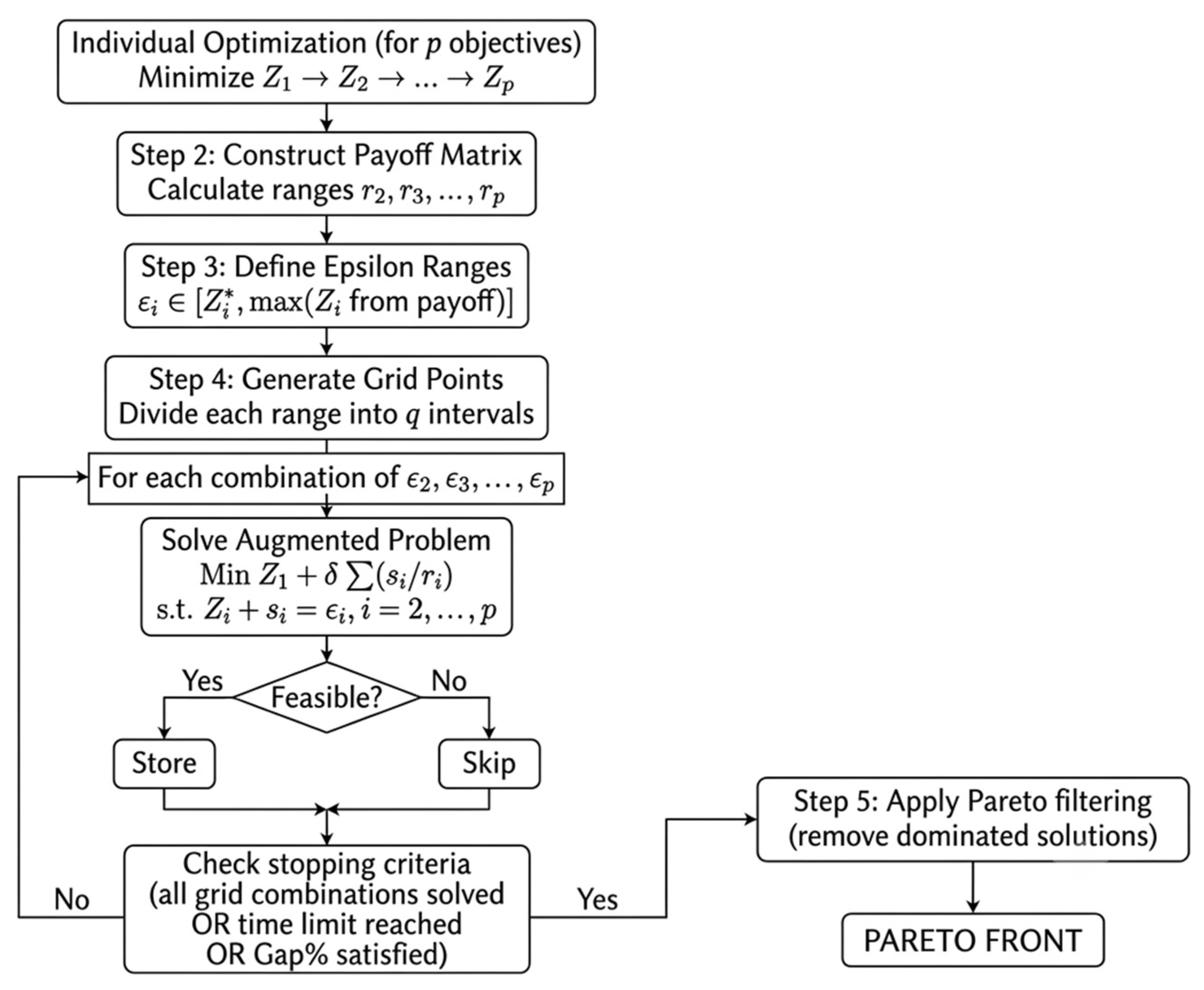
The AUGMECON method generates ε-optimal solutions for each ε-constraint subproblem, producing a discrete approximation of the Pareto front. All generated solutions are guaranteed to be Pareto-optimal (non-dominated) due to the augmented objective and slack variable formulation. Therefore, each Pareto point is globally optimal for its specific ε-constraint set, but the overall Pareto frontier is approximated due to the finite grid (5×5). The ε values and grid intervals were selected following the standard AUGMECON procedure. First, the individual minimum for each objective was obtained through single-objective optimization. Second, the maximum ε values were determined as the worst values across all individual optima, multiplied by safety factors to ensure the feasibility of all grid points. This safety margin guarantees that the entire ε range contains feasible solutions. Third, a 5 × 5 grid was selected, generating 25 ε-constraint subproblems. This grid provides sufficient resolution to capture the shape of the Pareto frontier while maintaining computational tractability, as recommended in the AUGMECON literature.

The solution procedure of the AUGMECON method is illustrated in Figure 3. The general formulation of the AUGMECON method is as follows:

$$\begin{array}{c}Minimize Z_1+ \delta \left({\displaystyle \frac{s_2}{r_2}}+{\displaystyle \frac{s_3}{r_3}}\right)\hfill \\ \mathrm{s}.\mathrm{t}.\hfill \\ \hfill Z_2+s_2={\epsilon }_2\hfill \\ \hfill Z_3+s_3={\epsilon }_3\hfill \\ \hfill \mathrm{x} \in \mathrm{X}{, s}_2, s_3\ge 0\hfill \end{array}$$

(57)

where

$\delta$ is a small positive number;

$s_2$ and $s_3$ are slack variables for the constrained objectives;

$r_2$ and $r_3$ are the ranges of objectives $Z_2$ and $Z_3$ respectively;

${\epsilon }_2$ and ${\epsilon }_3$ are parameters that define the right-hand side constraints.

The algorithm terminates when all grid points are evaluated. For each run, Gurobi stops with a 5% MIP gap or 3600 s time limit. After generating all solutions, a dominance check is performed to remove dominated solutions, keeping only non-dominated (Pareto-optimal) solutions.

6. Numerical Results

6.1. Model Validation and Case Study Description

The proposed multi-objective MILP model is first validated on a small-scale instance to verify its logical correctness and constraint formulations. The small-scale validation instance was constructed with reduced dimensions: two periods, two product types, two packaging options, three suppliers, two plants, two warehouses, two customers, and one transportation mode. This reduced instance was used to verify the logical correctness of all constraints. For this small instance, the model was solved to global optimality, and the solution was manually checked against expected logical behavior: all production was assigned to dedicated storage locations, no product was stored in non-dedicated locations, and tardiness occurred only when cumulative shipping times exceeded due dates. This step confirmed that the constraints were correctly formulated before scaling to the full industrial case. Subsequently, it is applied to a full-scale industrial case study based on real operational data from major steel manufacturers in Egypt. The case study is based on data from one of Egypt’s largest steel producers, which has an annual production capacity of 7 million tons of steel (4.7 million tons of long products and 2.3 million tons of hot-rolled coils). The company operates four production plants (using both DRI-EAF and scrap-based EAF routes). Three major distribution warehouses are considered and serve both domestic and export markets. All numerical parameters have been verified to represent realistic operational conditions. The full-scale problem corresponds to a tactical planning horizon of nine months, which reflects the typical medium-term planning cycle in the steel industry. The dimensions of the real-world case study are summarized in

Table 3. Dimensions of the Full-Scale Industrial Case Study.

Parameter	Description	Value
Nt	Planning periods (months)	9
Ni	Product types	2 (Long, Flat)
Nk	Packaging options	5
Ns	Suppliers	25
Nr	Raw material types	6
Np	Production plants	4
Nw	Warehouses	3
Nl	Storage locations per warehouse	30
Nc	Customers	2
Nm	Transportation modes	3 (Truck, Rail, Ship)
Nd	Collection centers	2
Nq	Scrap quality grades	3 (Premium, Standard, Low Grade)
Ne	Energy sources	3 (Natural gas, Electricity, Diesel)
Na	Water resources	2 (Desalinated, Fresh)

.

The industrial dataset was compiled by the authors from publicly available sources and industry reports, including financial statements, environmental disclosures, and operational benchmarks of major Egyptian steel producers. Some specific company data were estimated based on industry averages, technical literature, and Egyptian regulatory standards (e.g., Egyptian Environmental Affairs Agency, Egyptian Electricity Holding Company). All parameters were validated for consistency with real-world operating conditions. The resulting optimization model comprises approximately 450,000 decision variables reflecting the complexity of real-world steel supply chain operations. The AUGMECON method was applied with a 5 × 5 grid, generating 25 optimization runs for the full-scale problem. All experiments were executed using Python 3.10 with the Gurobi 13.0.1 solver on a laptop equipped with a 13th Gen Intel Core i7-13620H processor and 16 GB of RAM. The average runtime was approximately 484.7 s per run (ranging from 185 to 1299 s). All runs terminated with an optimality gap below 5% and indicated fast convergence. The reported runtime of 484.7 s (average) refers to a single AUGMECON subproblem solved with a 5% MIP gap. The complete Pareto frontier (5 × 5 grid) required approximately 12,000 s total across 25 runs.

6.2. Key Parameter Values

Table 4. Key parameter values for the full-scale case study.

Parameter	Description	Value/Range	Unit
BOM [scrap] [i]	Scrap ratio in EAF charge	0.20	ton/ton
BOM [iron ore] [i]	Iron ore (DRI feed)	0.586	ton/ton
Cpurch [Iron Ore]	Iron-ore purchase cost	4000–7500	EGP/ton
Cpurch [Scrap]	Steel scrap purchase cost	18,000–20,000	EGP/ton
Cpurch [Pitch Coke]	Pitch coke purchase cost	15,000–20,000	EGP/ton
Cpurch [Ferro-alloys]	Ferro-alloys purchase cost	57,000–60,000	EGP/ton
Cprod [Long]	Unit production cost (Long)	4800–6000	EGP/ton
Cprod [Flat]	Unit production cost (Flat)	5400–5700	EGP/ton
Cinv	Inventory holding cost	600–1200	EGP/ton/month
Cm [Truck]	Truck trip cost	20,000	EGP/trip
Cm [Rail]	Rail trip cost	120,000	EGP/trip
Cm [Ship]	Ship trip cost	900,000	EGP/trip
TC [Truck]	Truck capacity	25	Tons
TC [Rail]	Rail capacity	800	Tons
TC [Ship]	Ship capacity	2500	Tons
Epit [EAF + DRI]	Energy consumption	550	kWh/ton
Epit [EAF + scrap]	Energy consumption	420	kWh/ton
Cept [Electricity]	Industrial electricity cost	2.33	EGP/kWh
Cept [Natural Gas]	Natural gas cost	0.72	EGP/kWh
Apit	Water consumption	1.8–2.43	m3/ton
$\tau$	Scrap take-back rate	0.15	Fraction

presents the most significant parameter values used in the full-scale industrial case study. These values are derived from financial reports and industry standards, as well as validated through sensitivity analysis. The normalization ranges for transport emissions (truck, rail, and ship), energy emissions (natural gas, electricity, and diesel), and water impact (desalinated and fresh) were derived from literature values and official reports from Egyptian and international agencies. However, official reports typically provide single central values rather than minimum and maximum bounds. To construct the minimum and maximum bounds required for normalization, the lowest and highest values reported across multiple literature sources were adopted. This ensures the normalization ranges capture realistic variability in Egyptian operating conditions while remaining grounded in empirical data.

For parameters not listed in Table 4, values were generated within realistic ranges reported in the literature, industry databases, and the companies’ financial statements.

6.3. Individual Objective Minimum

Before generating the Pareto frontier, the model was solved for each objective individually to determine the minimum possible values.

Table 5. Individual objective minima.

Objective	Minimum Value	Cost (Billion EGP)	Tardiness (Months)	Emissions (Million_kg CO2)
Cost minimization	55,945,486,369.08	55.945	3.60	2072.18
Tardiness minimization	0.00	3142.28	0.00	2175.74
Emissions minimization	2,071,519,520.67	5237.61	3.60	2071.52

presents the individual minimum for the three objectives.

The cost-minimization solution achieves a total cost of 55.95 billion EGP with a tardiness of 3.60 months and emissions of 2072.18 million kg CO₂. The tardiness-minimization solution reduces tardiness to 0.00 months but increases cost dramatically to 3142.28 billion EGP (more than 56 times higher), while emissions rise slightly to 2175.74 million kg CO₂. The emissions-minimization solution achieves the lowest emissions at an extremely high cost of 5237.61 billion EGP, with tardiness remaining at 3.60 months. These results confirm the existence of severe trade-offs among the three objectives, particularly between cost and tardiness, as well as between cost and emissions. Such conflicting relationships motivate the need for a multi-objective optimization approach to identify balanced compromise solutions.

6.4. Pareto Front Results

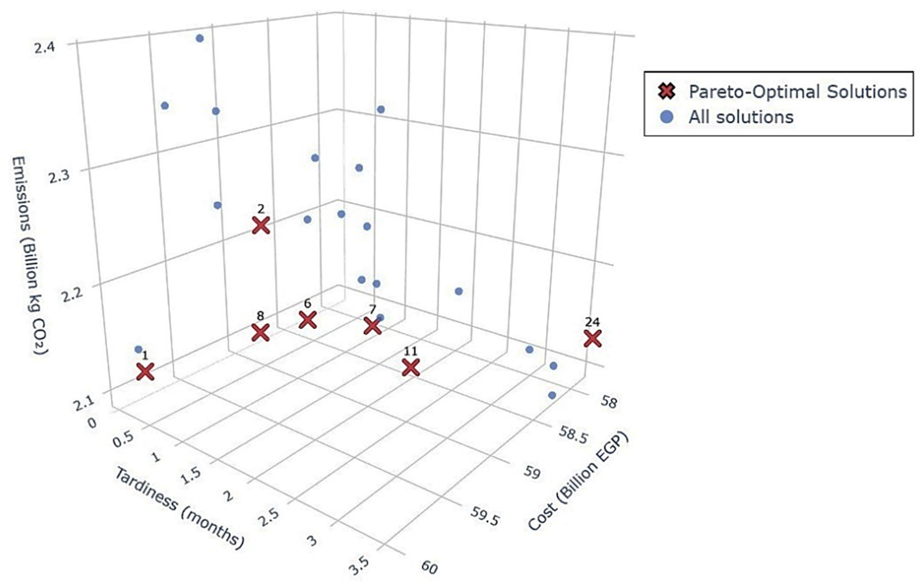
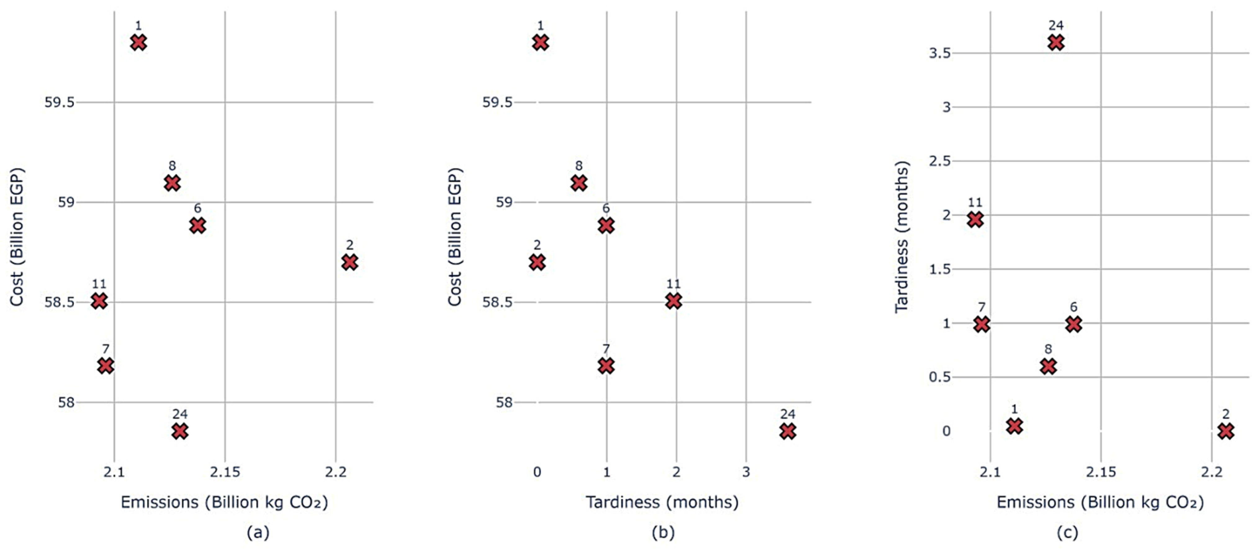
The AUGMECON method generated 25 solutions for the full-scale problem. After filtering dominated solutions, seven non-dominated solutions were identified, as presented in

Table 6. Pareto-optimal solutions (non-dominated) for the full-scale problem.

Solution ID	Cost (Billion EGP)	Tardiness (Months)	Emissions (Million kg CO2)	ε_Tardiness	ε_Emissions
24	57.86	3.600	2129.67	3.96	2,476,049,015
7	58.18	0.990	2096.13	0.99	2,206,362,685
11	58.51	1.960	2093.21	1.98	2,071,519,521
2	58.70	0.000	2206.36	0.00	2,206,362,685
6	58.89	0.990	2137.66	0.99	2,071,519,521
8	59.10	0.600	2126.20	0.99	2,341,205,850
1	59.80	0.048	2110.94	0.00	2,071,519,521

.

The Pareto frontier reveals that reducing tardiness from 3.60 months to 0.00 months increases total cost with a modest increase of 1.45%. Second, the zero-tardiness solution incurs higher emissions, revealing that perfect on-time delivery comes at an environmental cost. These results confirm that all three objectives exhibit meaningful trade-offs, but the cost-tardiness trade-off is more noticeable than the cost-emissions trade-off.

Figure 4 presents the 3D Pareto front showing the relationship among the three objectives. Figure 5 presents the Pareto trade-offs. The knee point, representing the best compromise solution among the three conflicting objectives, was identified using the normalized distance to the ideal point within the Pareto frontier. Solution 7 exhibits the smallest normalized distance to the ideal point (0.322), thus being selected as the recommended compromise solution offering near-optimal cost (only 0.55% above the absolute minimum), achieving excellent service level, and maintaining emissions close to the minimum achievable (only 0.14% above the absolute minimum).

6.5. Sensitivity Analysis

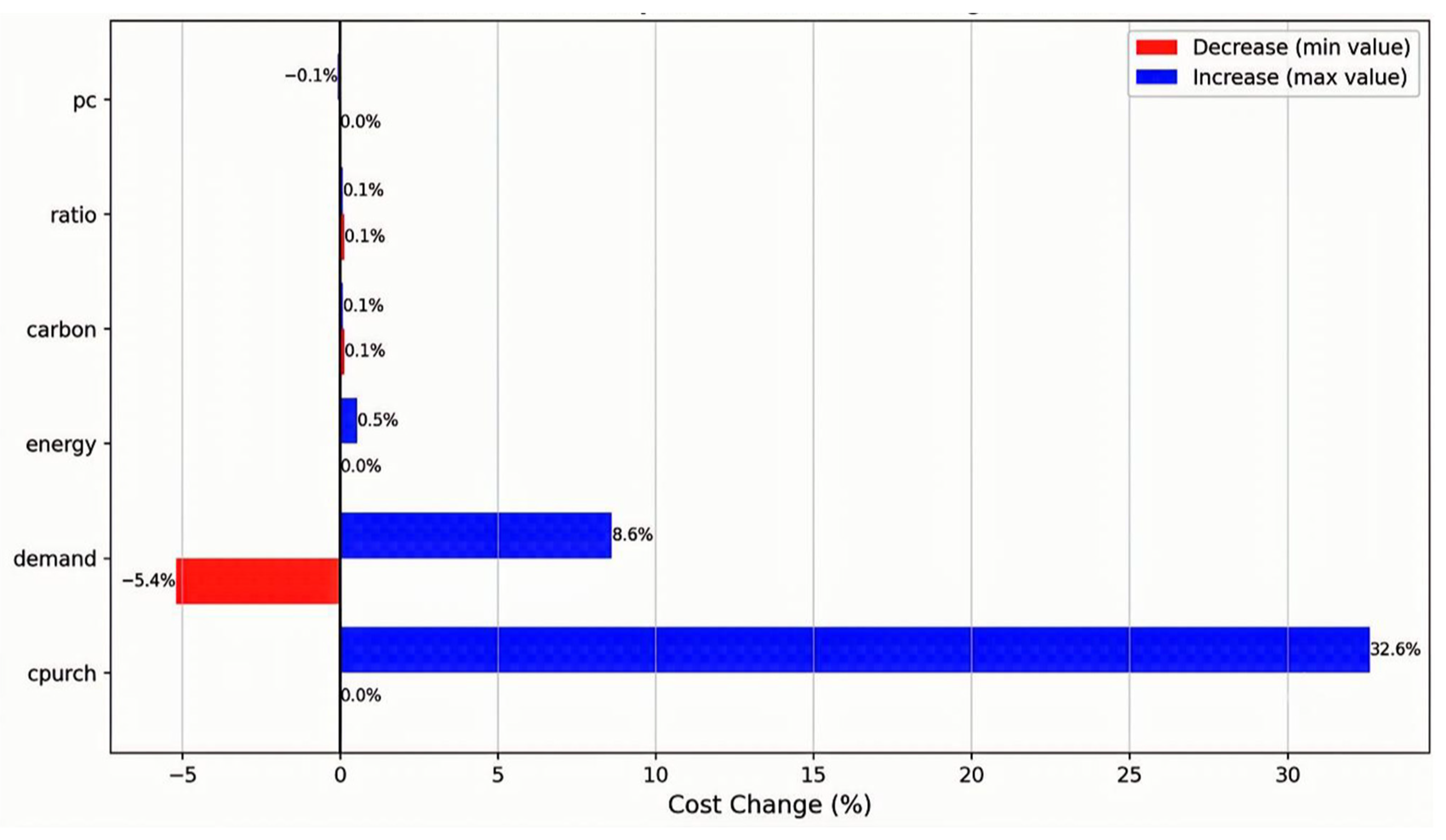
A sensitivity analysis is carried out to assess the robustness of the optimal solution and to understand how variations in key input parameters affect the three conflicting objectives: total cost, tardiness, and carbon emissions. The following parameters were examined due to their high uncertainty or strategic importance: raw material purchase price, demand variability, energy cost, production capacity, scrap take-back rate and carbon price. A one-factor-at-a-time (OAT) approach was implemented, where each parameter was varied across a reasonable range while all other parameters remained fixed at their baseline values. For each scenario, the multi-objective optimization was resolved using the AUGMECON method. Among the Pareto-optimal solutions, the one with the lowest cost was selected as the representative solution for that scenario. The corresponding cost, tardiness, emissions, and CPU time were recorded to evaluate the impact of parameter changes on problem difficulty. The tornado plot showing the sensitivity of the best Pareto-optimal cost is shown in Figure 6.

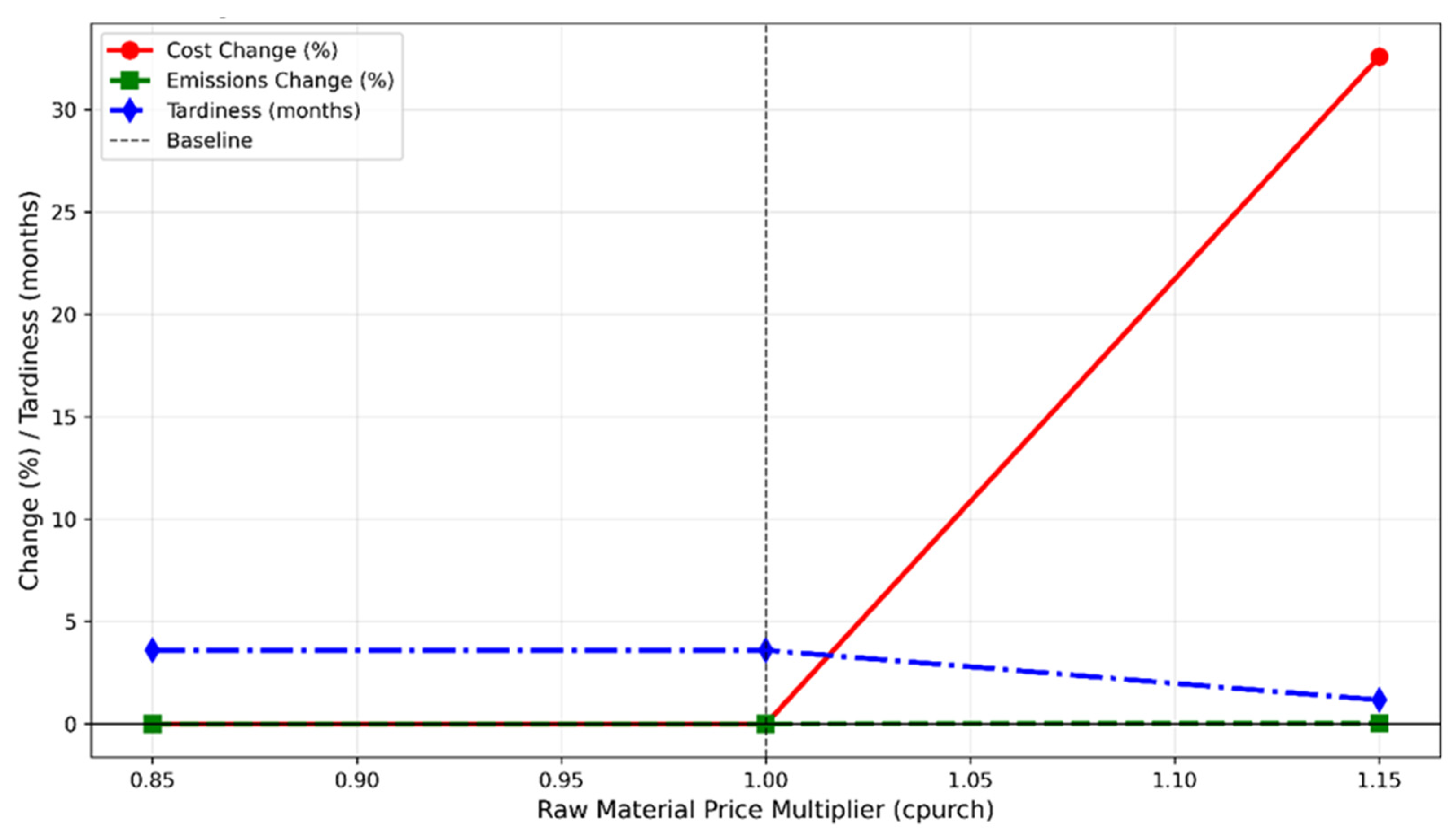
The results demonstrate that raw material purchase price and demand variability are the most influential parameters. A 15% increase in raw material purchase price raises best cost by over 32% (from 52.6 billion EGP to 69.8 billion EGP), while tardiness improves to 1.17 months. Emissions remain virtually unchanged (<0.1%). In contrast, carbon tax, energy cost, production capacity, and scrap take-back rate have effects within ±1%, indicating low sensitivity.

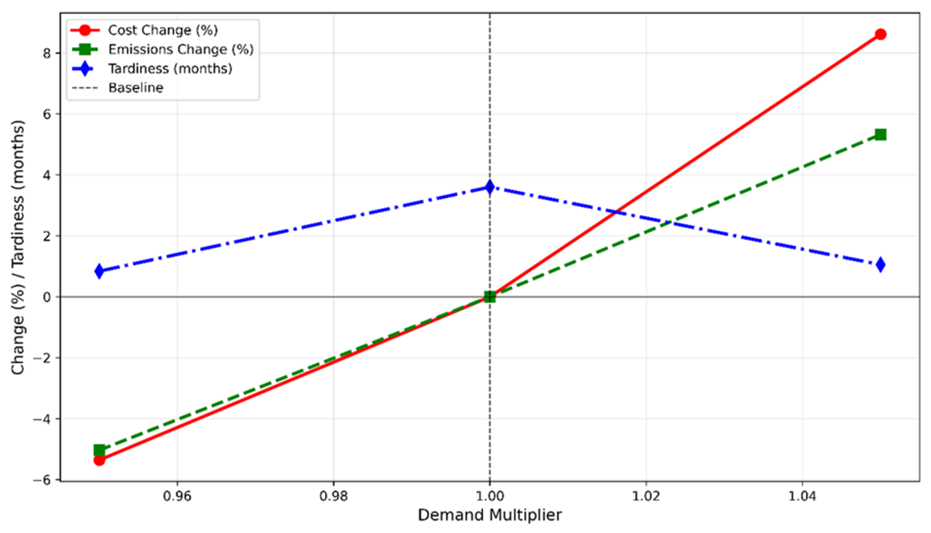
Demand variability is the only parameter that significantly affects all three objectives. A 5% decrease in demand improves tardiness by 76.7% (from 3.60 to 0.84 months) and reduces emissions by 5.03%, while a 5% demand increase raises emissions by 5.32% and increases the cost by 8.6% while improving tardiness to 1.05 months.

Raw material price and demand variability scenarios require the highest computational effort (up to 3182 s), while carbon tax scenarios are the fastest (as low as 1562 s).

Table 7. Sensitivity summary (Pareto-optimal framework).

Parameter	Cost Sensitivity	Tardiness Sensitivity	Emissions Sensitivity	CPU Time Sensitivity
Raw material price	High (+32.6%)	Moderate (2.4)	Negligible (<0.1%)	High (3182 s)
Demand variability	High (+8.6%/−5.4%)	High (2.7)	High (5.3%)	High (3154 s)
Energy price	Low (<±1%)	Moderate (2.4)	Negligible (<0.1%)	Moderate (2325 s)
Production Capacity	Low (<±1%)	$\mathrm{Negligible} (\approx 0$)	Negligible (<0.1%)	Moderate (2319 s)
Carbon price	Low (<±1%)	$\mathrm{Negligible} (\approx 0$)	Negligible (<0.1%)	Low (2183 s)
Take-back ratio	Low (<±1%)	$\mathrm{Negligible} (\approx 0$)	Negligible (<0.1%)	Moderate (2606 s)

Numerical values in parentheses represent the maximum absolute percentage change in cost, maximum absolute change in tardiness (months), maximum absolute percentage change in emissions, and maximum CPU time (seconds), respectively.

provides a consolidated summary of the sensitivity of each objective to each parameter under the Pareto-optimal framework.

The most critical parameters for multi-objective decision-making are raw material purchase price and demand variability, as they strongly influence all three objectives and computational time within the Pareto frontier. Energy cost, production capacity, carbon tax, and scrap take-back rate have limited impact under current conditions, suggesting that management attention should focus on supply chain and demand management rather than on energy or environmental policy in the short term. However, as industry transitions toward low-carbon technologies, the sensitivity to energy cost and carbon tax may increase substantially, potentially reshaping the Pareto frontier.

Figure 7 and Figure 8 illustrate the impact of demand variability and raw material price. Demand variability affects all three objectives. The strong influence of demand variability on cost and tardiness is consistent with the well-known bullwhip effect, where small fluctuations in customer demand are amplified upstream, leading to higher inventory and production costs. In contrast, raw material prices strongly affect cost but have a negligible impact on emissions (<0.1%) and affect tardiness only at the highest price level.

7. Discussion

As established in Section 4, the three objectives (cost, tardiness, and emissions) are naturally conflicting. This section interprets the numerical results, focusing on how circular economy and key operational parameters affect steel supply chain performance.

The results of this research clearly demonstrate that the three objectives—cost, tardiness, and carbon emissions—are inherently contradictory. These findings are consistent with Askary et al. [3], who reported significant trade-offs between cost and environmental objectives, and Khalili-Fard et al. [4], who highlighted the conflicting nature of cost and emissions under circular economy policies. The AUGMECON method successfully generated 25 solutions, of which seven were Pareto-optimal. The Pareto frontier revealed meaningful trade-offs: reducing tardiness from 3.60 to 0.00 months increased total cost by 1.45%, indicating that near-perfect service levels can be achieved at a remarkably low economic cost in the steel industry. Conversely, minimizing emissions to 2071.52 million kg CO₂ came at an extremely high cost, confirming that deep decarbonization is not achievable through operational adjustments alone under current technology.

The knee point was selected as the best compromise, with a cost of 58.18 billion EGP, tardiness of 0.99 months, and emissions of 2096.13 million kg CO₂. Its normalized distance to the ideal point is 0.322, which reflects a balanced trade-off where no objective can be substantially improved without sacrificing another. Compared to the lowest-cost solution, the knee point reduces tardiness by 72.5% with a 0.55% cost increase. Compared to the lowest-emissions solution, it achieves virtually identical emissions (0.14% higher) with 0.56% lower cost and 49.5% lower tardiness. Thus, the knee point provides managers with a practical compromise that prioritizes service level and cost efficiency while keeping emissions close to the minimum achievable.

Although the knee point solution provides a mathematically balanced compromise, managerial choices among Pareto optimal solutions ultimately depend on the strategic priorities of the firm. For instance:

• If a steel manufacturer prioritizes cost minimization above all else, Solution 24 (57.86 billion EGP) would be preferred despite its high tardiness (3.60 months).
• If service level is the dominant objective, Solution 2 (zero tardiness) becomes attractive, albeit at a higher cost (58.70 billion EGP) and increased emissions (2206.36 million kg CO₂).
• For decision makers who emphasize environmental performance, Solution 11 offers the lowest emissions (2093.21 million kg CO₂) while maintaining reasonable cost and tardiness.

To facilitate this selection process, the Pareto frontier reported in Table 6 can be used interactively: managers first define their primary objective, then identify the corresponding extreme solution, and finally navigate along the frontier to a solution that satisfies secondary constraints (e.g., maximum acceptable cost or maximum tolerable tardiness).

The knee point solution serves as a natural starting point for this exploration because it represents the best compromise when no single objective is prioritized. This practical approach bridges the gap between abstract Pareto optimality and actionable strategic planning in the steel industry.

The sensitivity analysis further highlighted the critical parameters for decision-making. Raw material purchase price and demand variability are the most influential: a 15% increase in raw material purchase price raises the best cost by over 32%, while a 5% demand increase raises cost by 8.6%. Interestingly, emissions are only sensitive to demand volume, confirming that emissions are primarily determined by production volume under current technology. Carbon tax, energy cost, production capacity, and scrap take-back rate have negligible effects (within ±1%), indicating that carbon pricing alone (e.g., a carbon tax) cannot drive deep decarbonization without complementary technological breakthroughs, such as hydrogen-based DRI or carbon capture and storage.

The dominance of raw material price and demand variability over carbon tax and scrap take-back can be explained by the current technology and market context. First, under existing EAF-DRI technology, carbon emissions are primarily determined by production volume rather than carbon pricing, as energy sources (natural gas, electricity) are already optimized. A carbon tax of typical magnitudes represents less than 2% of total production cost, whereas raw materials account for 60–70% of steelmaking costs. Second, the scrap take-back rate is currently limited due to collection constraints and scrap quality issues; increasing this rate would require investment in sorting and processing facilities, which are not captured in short-term operational models. Therefore, in the current industrial context, raw material cost and demand fluctuations drive performance more strongly than environmental policies or circular economy practices.

The sensitivity analysis shows that a 15% increase in raw material price raises total cost by over 32%, making raw material price the most critical risk factor. To mitigate this risk, steel plant managers should consider:

• Long-term contracts with key suppliers to stabilize prices.
• Supplier diversification to reduce dependency on single sources.
• Strategic stockpiling of critical raw materials (e.g., iron ore, scrap) during low-price periods.
• Hedging strategies using commodity futures, if available.

These strategies can help decouple supply chain performance from short-term price volatility.

Despite the central emphasis on circular economy practices in sustainable supply chain literature, increasing the scrap take-back rate from 0% to 15% in this study resulted in only a marginal performance improvement (less than 0.3% cost reduction and no significant change in emissions or tardiness). This limited impact can be attributed to three key factors specific to the Egyptian steelmaking context.

First, baseline production already incorporates a substantial proportion of scrap (approximately 20% in the EAF charge) together with high-quality direct reduced iron (DRI), so that an additional 15% take-back substitutes one raw material for another without fundamentally altering the production route.

Second, the purchase price of scrap is relatively high compared to DRI, eroding any potential cost advantage.

Third, under the current energy mix (natural gas-based DRI), the emission factor of scrap-based EAF melting is only moderately lower than that of DRI-based production, so the reduction in CO₂ emissions remains marginal.

Consequently, while circular economy principles are conceptually desirable, their real-world effectiveness in the Egyptian steel sector remains constrained by existing technology, relative prices, and the already high baseline scrap utilization. This finding underscores that achieving deep decarbonization will require not only higher take-back rates but also complementary breakthroughs such as hydrogen-based DRI or carbon capture and storage.

Regarding water ecological effects, the results show that water accounts for less than 5% of the total normalized environmental impact in the knee point solution (solution 7). This low contribution can be explained by the specific operational context of the Egyptian steel plant studied, which employs closed-loop water recirculation systems that achieve approximately 95–98% water reuse—a common practice in modern steel facilities to comply with local environmental regulations. Nevertheless, in water-stressed regions like Egypt, water impacts could become a dominant concern for steel plants operating older once-through cooling systems, where water withdrawal and discharge volumes are substantially higher. The proposed model is flexible and can be adapted to assign higher weights to water ecological effects if local conditions or regulatory priorities require such emphasis. This adaptability is an important feature for policymakers and plant managers in water-scarce regions.

These results offer several managerial implications for steel supply chain planning. First, managing raw material prices should be a top priority, as price increases can drastically reduce profitability. Long-term contracts, supplier expansion, and strategic stockpiling are recommended. Second, demand forecasting accuracy is critical for both cost and service level performance; investments in demand sensing technologies and flexible capacity are more effective than holding excess inventory. Third, carbon pricing alone is insufficient to reduce emissions under current EAF-DRI technology; complementary policies such as subsidies for hydrogen-based DRI or carbon capture are necessary. Fourth, circular economy practices (scrap take-back) have limited short-term impact, but managers should monitor scrap prices and carbon taxes as these may reshape the Pareto frontier in the future.

The proposed framework can support Industry 4.0 and Industry 5.0 transformations in steel manufacturing. First, the model’s sensitivity analysis identifies demand variability as a key driver, which can be addressed through Industry 4.0 technologies such as real-time demand sensing, IoT-enabled inventory tracking, and AI-based demand forecasting. Second, the Pareto frontier provides decision support for human-centric (Industry 5.0) manufacturing, where managers select compromise solutions balancing cost, service level, and environmental impact—reflecting the Industry 5.0 principle of human–machine collaboration. Third, the model’s structure allows integration with digital twins for scenario analysis and real-time replanning. Future work could incorporate real-time data streams from smart warehouses and predictive analytics for adaptive supply chain optimization under the Industry 5.0 paradigm.

The current research could guide managers in decision-making and strategic planning in several directions. In line with many scholars, the environmental and social dimensions of the supply chain affect the configuration of the closed-loop supply chain. Improving distribution planning by including sustainable goals, as derived from the proposed model, is also a strategic decision for enhancing corporate social responsibility. Moreover, the results show that a proper balance between long-term and short-term goals should be created. Managers who can finance more facilities in the initial stages (e.g., expanding production capacity) exhibit higher performance in all sustainability goals. Meanwhile, if the supply chain is equipped with appropriate flexibility strategies, it will respond better to business changes such as demand fluctuations; otherwise, it will be forced to sacrifice some sustainability indicators for others. Nevertheless, this study has some limitations. First, demand, processing times, and travel times are treated as deterministic, whereas real-world steel supply chains face significant uncertainty. Future work could extend the model using robust optimization or stochastic programming. Second, the case study is based on a single Egyptian steel manufacturer, which may limit generalizability to other regions or production technologies. However, the methodology is transferable, and the sensitivity analysis provides insights applicable to similar contexts. Third, the 5 × 5 ε grid may not capture all trade-offs on the Pareto frontier; a finer grid would improve resolution at higher computational time. Fourth, while key parameters were derived from real operational data and validated against market reports, some input values (e.g., specific energy consumption per product type, exact water recirculation rates) relied on industry averages and literature rather than site-specific measurements. Fifth, scalability to enterprise-level planning may require decomposition techniques or metaheuristics.

8. Conclusions

This study investigated, using a real-world case study of a major Egyptian steel manufacturer under a dedicated warehousing policy, how circular economy practices and key operational parameters affect the trade-offs among total cost, order tardiness, and CO₂ emissions. The model presented in this work optimizes three conflicting objectives: total economic cost, including fixed, transportation, production, inventory, energy, and purchasing costs; service level measured as total tardiness; and finally, the environmental effects measured as carbon emissions. The concept of circular economy is integrated through a scrap take-back rate, where scrap is incorporated in the production process. The model was validated on a real-world case study of major Egyptian steel manufacturers. The AUGMECON (augmented ε-constraint) method with a 5 × 5 grid is used to generate Pareto-optimal solutions.

The numerical results showed significant trade-offs among the three objectives. Seven non-dominated solutions generated from 25 simulations developed the Pareto frontier. The knee-point solution (58.18 billion EGP, 0.99 months tardiness, and 2096.13 million kg CO₂) improves tardiness by 72.5% with only a 0.55% cost increase compared to the lowest-cost solution. On the other hand, when compared to the lowest-emissions solution, the knee point solution achieves nearly the same emissions (0.14% higher) with 0.56% lower cost and 49.5% lower tardiness. These results demonstrate that excellent service levels can be achieved with small cost increases.

Methodologically, this study advances integrated sustainable steel supply chain optimization in three ways. First, it presents a unified multi-objective MILP framework that simultaneously captures production, packaging, warehousing (with dedicated storage location assignments), multi-modal transportation, energy and water consumption, and reverse scrap flows—an integration rarely attempted in a single tactical planning model. Second, it demonstrates that the augmented ε constraint (AUGMECON) method can be effectively applied to a real-world problem with approximately 450,000 decision variables, generating a well-distributed Pareto frontier and identifying a knee point compromise solution without requiring subjective weighting of objectives. Third, by embedding one factor at a time (OAT) sensitivity analysis within the multi-objective framework, the study offers a replicable methodology to assess how external parameter uncertainties (demand, raw material price, energy cost, carbon tax, and scrap take-back rate) affect the entire trade-off front, not just a single optimal solution. This methodological framework can be readily adapted to other energy-intensive supply chains (e.g., aluminum and cement) or extended to include additional sustainability dimensions.

One-factor-at-a-time sensitivity analysis was conducted on six key parameters: raw material purchase price, demand variability, energy cost, production capacity, carbon tax, and scrap take-back rate. The analysis showed that raw material purchase price and demand are the most significant parameters. A 15% increase in raw material purchase price raises the best Pareto-optimal cost by over 32%, while a 5% demand increase raises cost by 8.6%. Demand variability also strongly affects tardiness (a 5% demand decrease improves tardiness by 76.7%) and emissions (5.03% reduction). On the other hand, carbon tax, energy cost, production capacity, and scrap take-back rate have effects within ±1%, indicating low sensitivity. Carbon tax does not reduce emissions under current technology, highlighting the need for complementary investment policies.

Several important managerial insights can be drawn. First, the raw material price risk management and demand forecast accuracy should be top priorities. Second, carbon pricing alone is insufficient for the successful decarbonization of the steel industry; support for hydrogen-based DRI is necessary. Third, circular economy (scrap take-back) currently has a limited short-term impact on the system under consideration, but further investigation is needed, particularly related to the development of scrap prices and carbon taxes.

Some limitations should be acknowledged, including deterministic assumptions, single-case generalizability, data availability constraints, and computational scalability challenges as discussed in Section 7. For future research, several directions are recommended. First, alternative storage policies (e.g., class-based and random storage) could be explored to assess their impact on cost, service level, and environmental performance. Second, extending the deterministic framework to stochastic or robust optimization would capture demand, supply, and lead time uncertainties. Third, finer ε grids or alternative multi-objective methods (e.g., goal programming and compromise programming) could be explored. Fourth, the integration of real-time digital monitoring and Industry 5.0 technologies—such as AI-enabled adaptive production planning and smart warehousing systems—would enable dynamic re-optimization under changing conditions [26,27]. Fifth, hybrid solution approaches combining exact methods with metaheuristics could enhance scalability for larger problem instances. Sixth, incorporating circular economy principles more deeply (e.g., quality degradation across multiple recycling loops, carbon credit trading) and integrating life cycle assessment (LCA) for upstream and downstream emissions would further enrich the environmental analysis. Seventh, future studies should extend this work by comparing the proposed integrated model against baseline scenarios without circular economy provisions or with alternative warehousing policies (e.g., shared or randomized storage) to quantify the marginal benefits of each policy element.