
An Integrated Optimisation Model for LNG Supply Chain Planning and Infrastructure Under FOB Scheme with Time-Dependent Demand


Abstract
1. Introduction
2. Literature Review
2.1. LNG Supply Chain Planning and Small-Scale LNG Logistics
2.2. Hub-and-Spoke Network and Archipelagic LNG Distribution Networks
2.3. Optimisation Framework for LNG Transportation and Infrastructure Design
2.4. Contractual Arrangements and Buyer-Controlled LNG Logistics
2.5. Long-Term Planning and Demand Evolution in LNG Supply Chains
2.6. Research Gap and Contribution Positioning
3. Problem Description and Decision Framework
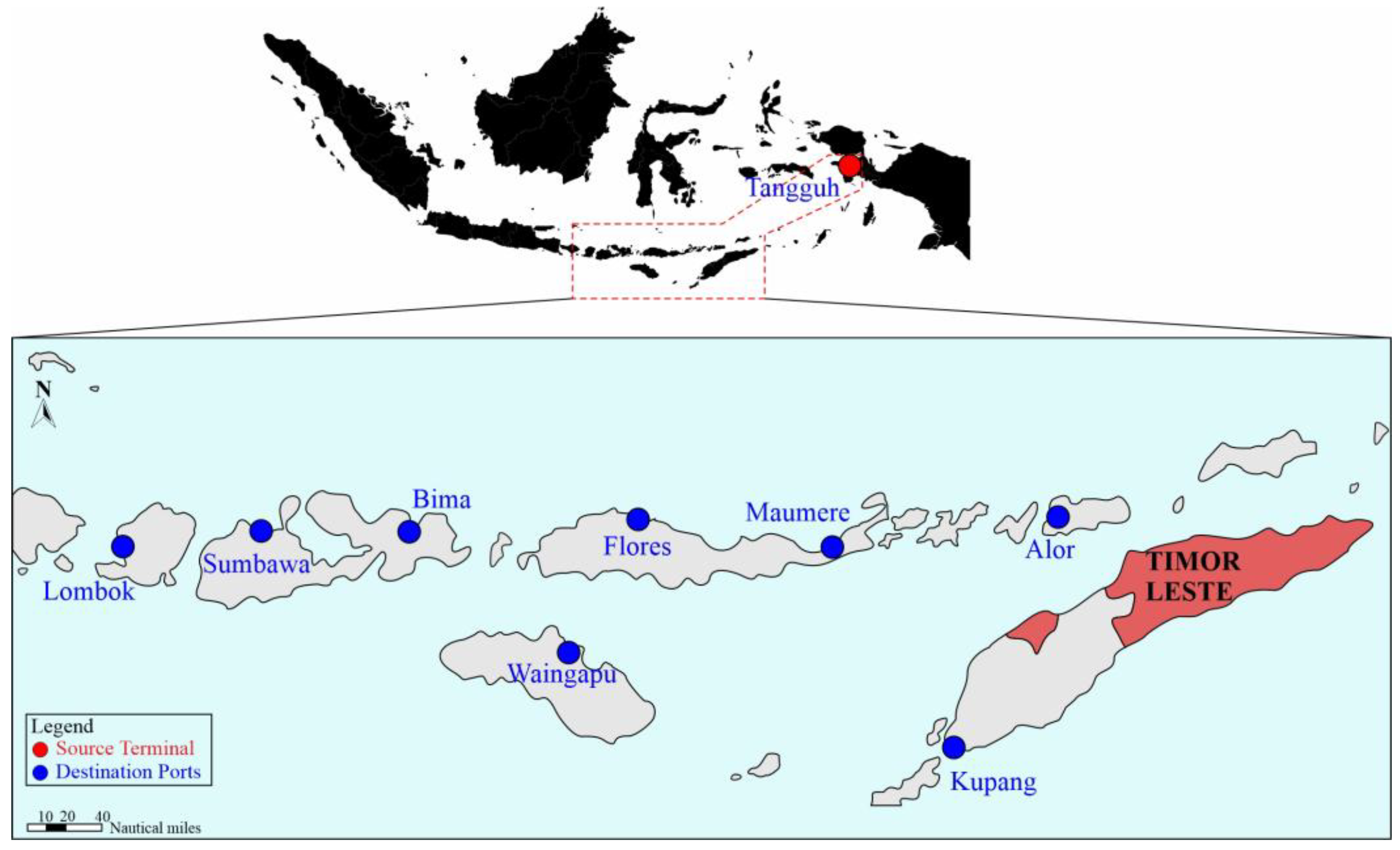
3.1. System Description
3.2. Decision Variables and Planning Scope
- Hub selection: Identifying the most cost-efficient destination port to serve as the regional LNG hub.
- Port clustering: Assigning each non-hub port to a downstream cluster served from the hub, ensuring that each port is exclusively assigned to a single cluster.
- Fleet configuration: Determining vessel capacity and fleet size for both upstream and downstream transportation segments.
- Routing: Optimising sailing routes within each downstream cluster.
3.3. Model Positioning: Strategic Versus Operational Planning
3.4. Model Assumptions and Justification
- Single LNG source terminal: LNG supply availability is assumed to be unconstrained, while operational service capacity is explicitly limited in terms of vessel call frequency.
- FOB contractual scheme: All transportation responsibilities and associated costs from the source terminal to the destination ports are borne by the buyer, enabling full end-to-end optimisation.
- Deterministic time-dependent demand: Demand at each port is assumed to be known and varies deterministically over time, allowing for the systematic evaluation of capacity adequacy over a long-term planning horizon.
- Hub-and-spoke network structure: One destination port is selected as a hub to consolidate upstream shipments and redistribute LNG to spoke ports as well as to meet local demand.
- Exclusive clustering: Each non-hub port is assigned to only one downstream cluster to avoid fragmented logistics operations.
- Uniform vessel size per segment: The upstream segment and each downstream cluster are served by vessels of identical capacity. This assumption reflects long-term time-charter practises and avoids excessive fleet fragmentation at the strategic level.
- Continuous annual operations: The logistics system is assumed to operate continuously throughout the year. As justified in Section 3.3, stochastic interruptions and maintenance downtime are abstracted to preserve model tractability.
- Neglect of boil-off gas: Boil-off gas (BOG) dynamics are not explicitly modelled, as their impact on strategic network configuration and infrastructure sizing is considered secondary relative to dominant transportation and investment cost drivers. In several maritime supply chain models, BOG is implicitly treated as an operational parameter rather than a separate material flow, and in some cases, the vaporised LNG is assumed to be used for onboard power generation. Consequently, the direct financial impact of BOG is absorbed into aggregated operating cost parameters rather than modelled explicitly as an independent cost component [29,30].
4. Model Formulation and Solution Approach
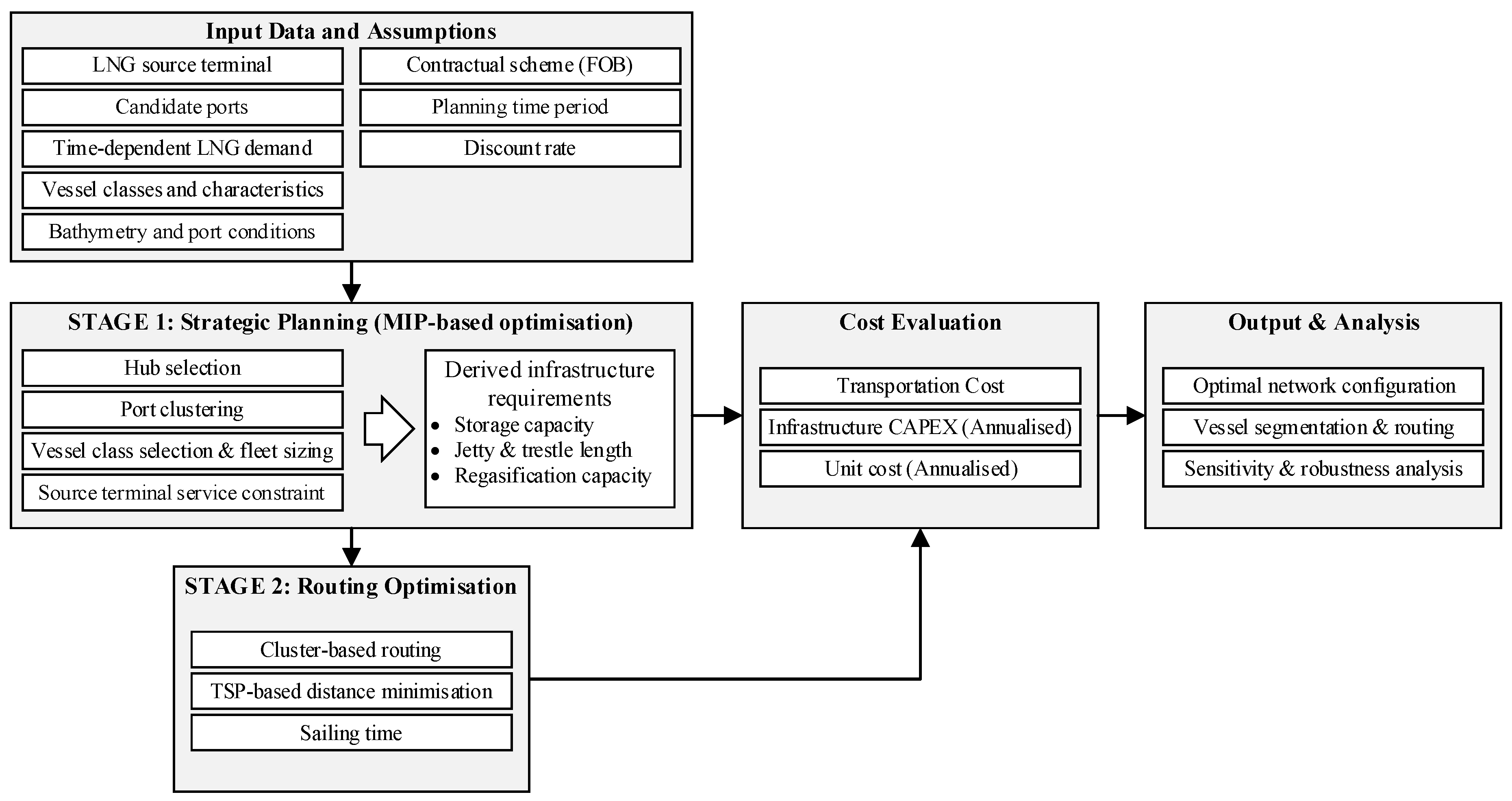
4.1. Overview of the Optimisation Framework
4.2. Symbol Explanation
4.3. Stage 1: Strategic-Level Optimisation
4.3.1. Network Structure
4.3.2. Vessel Class Representation and Fleet Configuration
4.3.3. Source Terminal Service Capacity Constraint
4.3.4. Infrastructure Sizing Logic
4.3.5. Mathematical Model
- The selection of a single hub port from a set of candidate destination ports.
- The assignment of non-hub ports into downstream clusters served from the hub.
- Vessel size classes and fleet sizes for upstream (source-hub) and downstream (hub-spoke) transportation.
- The resulting infrastructure capacity requirements at hub and spoke ports.
4.4. Stage 2: Operational Routing Optimisation
4.5. Cost Evaluation Framework
4.5.1. Infrastructure-Related Costs
- Infrastructure CAPEX: Includes initial investments in storage tanks, jetties, including trestles, and regasification units at both hub and non-hub ports. As described in Section 4.3.4, these capacities are derived endogenously based on the selected logistics configuration, vessel characteristics, bathymetric conditions, and peak demand requirements. To integrate with annual expenses, CAPEX is converted to an equivalent uniform annual cost using the capital recovery factor (CRF).
- Infrastructure O&M: Represents annual upkeep costs, modelled as a fixed percentage of the total infrastructure investment. This pragmatic assumption captures recurring facility expenses without introducing excessive operational complexity.
4.5.2. Transportation Costs (OPEX)
- Time Charter Costs (Fixed): Correspond to the annual cost of fleet deployment, determined by the number of vessels (upstream and downstream) selected in Stage 1 and the market charter rates for the respective vessel classes.
- Voyage Costs (Variable): Include fuel consumption, port charges, and anchorage fees. Fuel consumption is calculated across distinct operating states: (i) loading, (ii) discharging, (iii) sailing, and (iv) idle/anchorage. Port charges depend on call frequency, while anchorage costs are driven by accumulated idle time. These variables are directly derived from the routing outcomes in Stage 2.
4.5.3. Unit Cost Aggregation
4.6. Solution Approach
4.7. Model Scope and Limitations
- Deterministic Demand: LNG demand at each destination port is represented using a deterministic, time-dependent profile. This approach enables the systematic evaluation of capacity adequacy and infrastructure requirements under peak-demand conditions, which are critical drivers of long-term investment decisions. While demand uncertainty is not explicitly modelled, the robustness of the resulting network configuration is examined through sensitivity analysis, as discussed in Section 6.6.
- Exclusion of Boil-off Gas (BOG): BOG losses during transportation and storage are not explicitly incorporated into the cost formulation. As justified in Section 3.4, this simplification is consistent with the study’s strategic objective. Given that BOG costs are secondary to dominant transportation and infrastructure (CAPEX) cost drivers, excluding them helps isolate the structural effects of logistics configuration without significantly altering the optimal network topology. Advanced studies on BOG dynamics demonstrate that an accurate representation requires nonlinear thermal modelling and dynamic simulation [33,34]. Incorporating such non-linear and ship-specific thermodynamic behaviour into the supply chain optimisation framework would significantly increase computational complexity and reduce model tractability.
- Operational Abstraction: The model abstracts from detailed operational constraints such as daily berth scheduling, specific time windows, weather-related disruptions, maintenance downtime, and short-term fleet dispatching. These factors are more relevant to operational-level optimisation and vessel performance analysis than to long-term network design. By excluding such constraints, the framework preserves analytical clarity and focuses on decisions with long-term, irreversible economic implications.
- Solution Optimality: Regarding the solution methodology, it is acknowledged that the Genetic Algorithm (GA)-based approach identifies the best solution found within the search space rather than a mathematically proven global optimum. This limitation is common in strategic logistics optimisation studies employing metaheuristics for large-scale combinatorial problems. Future research may address this by comparing GA-based solutions against exact Mixed-Integer Programming (MIP) formulations (for smaller instances), decomposition-based methods, or alternative metaheuristics to further validate solution quality.
5. Case Study and Data
5.1. Case Study Background
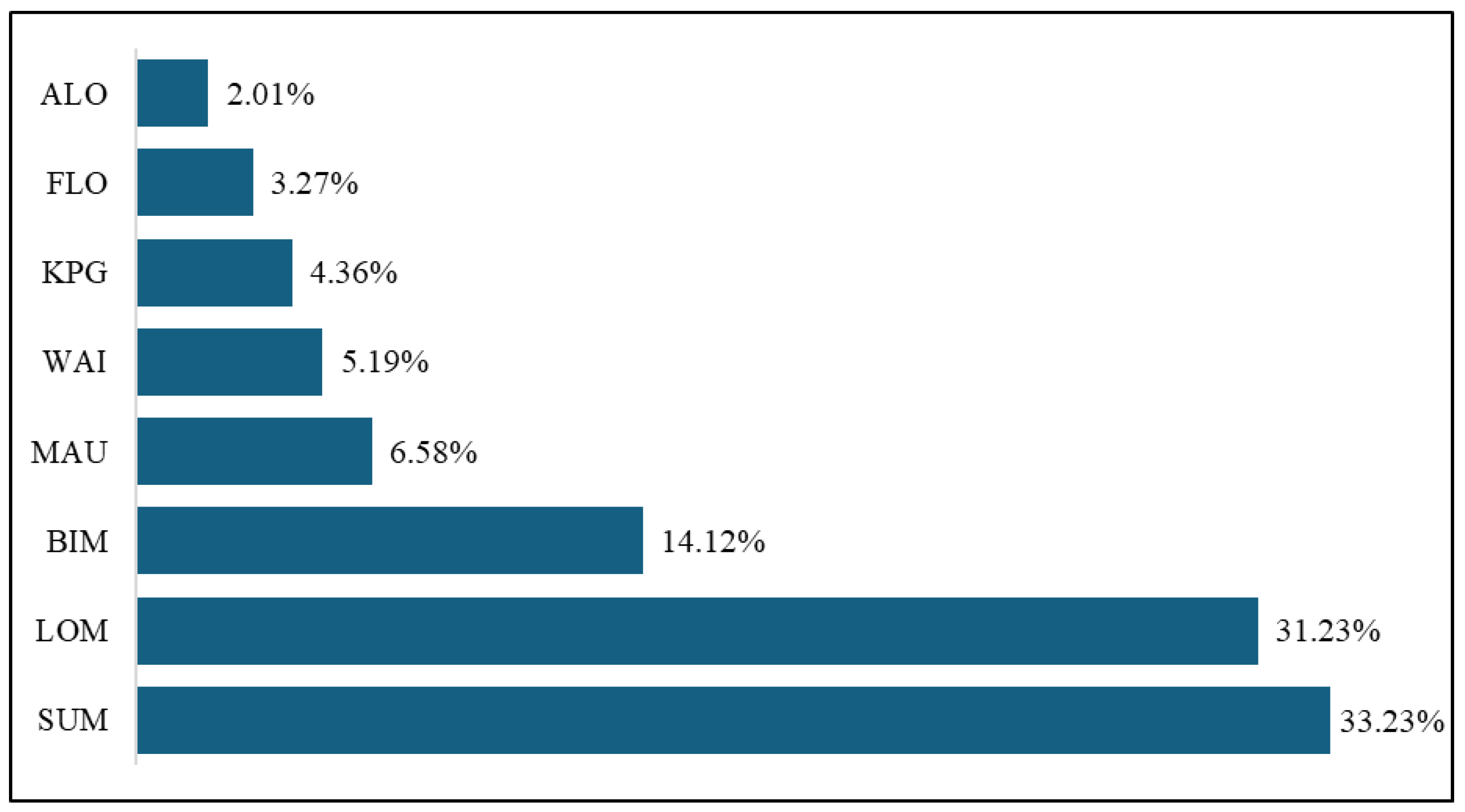
5.2. Demand Profile and Growth Assumptions
5.3. Vessel Sizes and Cost Parameters
5.4. Logistics Infrastructure Parameters
5.4.1. Storage Facilities
5.4.2. Marine Infrastructure (Jetty and Trestle)
5.4.3. Regasification and O&M
5.5. Economic and Operational Settings
6. Results
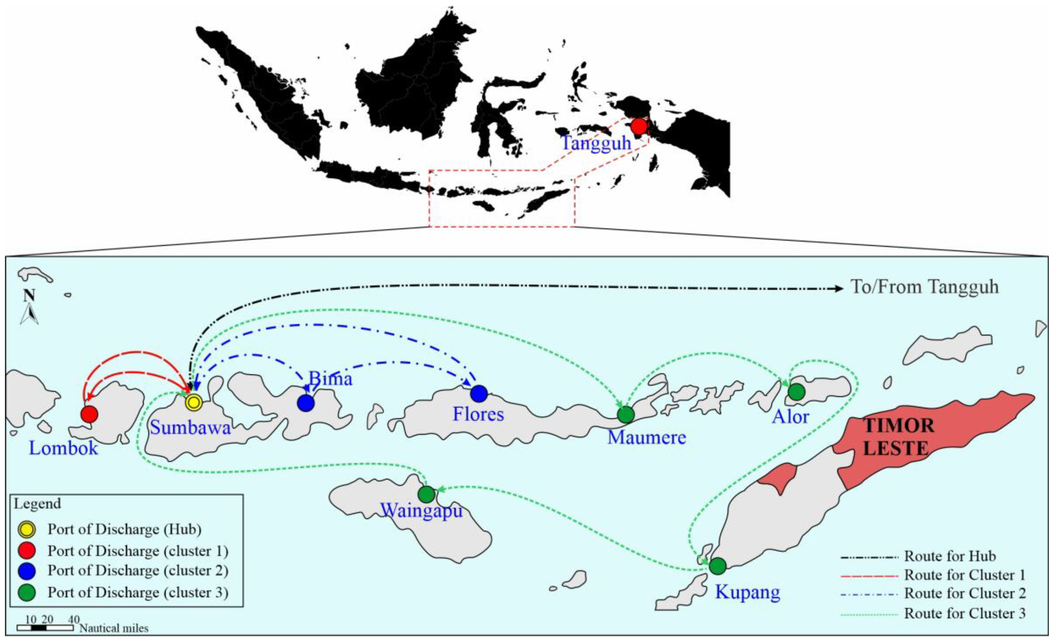
6.1. Optimal Network Configuration
- Cluster 1: LOM
- Cluster 2: BIM, FLO
- Cluster 3: KPG, MAU, ALO, WAI
6.2. Vessel Configuration and Operational Performance
6.2.1. Upstream Fleet Selection
6.2.2. Downstream Fleet Configuration
- Cluster 1 (LOM) is served by a 3500 m3 vessel class. Despite Lombok’s relatively high demand, its short sailing distance from the SBW hub enables high service frequency with smaller vessels while maintaining acceptable berth utilisation and transportation cost efficiency.
- Cluster 2 (BIM and FLO) is also served by 3500 m3 vessels. The combined demand of these two ports does not justify the deployment of larger vessels when evaluated against sailing distances and charter costs. The model prioritises maintaining high utilisation levels while avoiding excess capacity.
- Cluster 3 (MAU, ALO, KPG, and WAI) is served by a 10,000 m3 vessel class. Although individual demand levels at these eastern ports are relatively moderate, their geographic dispersion and longer sailing distances from the hub increase round-trip cycle time. Aggregating these nodes into a single cluster with a larger vessel reduces required voyage frequency and improves cost efficiency over long-haul downstream distribution.
6.2.3. Dynamic Fleet Expansion
6.3. Operational Routing Optimisation Results
6.3.1. Route Efficiency and Sailing Distances
- Upstream route: The dedicated shuttle service between the Tangguh source and Sumbawa hub covers a round-trip distance of 2086 nm. Given the long-haul leg, a large 65,000 m3 carrier is necessary to ensure economic viability while meeting the service capacity constraint at the source terminal.
- Cluster 1: As cluster 1 comprises only a single port, the routing problem is trivial; therefore, explicit sailing distance minimisation is not required for this cluster.
- Cluster 2: The route SBW ⟶ BIM ⟶ FLO ⟶ SBW covers 500 nm. Although longer than Cluster 1, this medium-range loop remains compatible with the 3500 m3 vessel class, balancing sailing time and cargo aggregation without requiring larger parcel sizes.
- Cluster 3: The eastern cluster SBW ⟶ MAU ⟶ ALO ⟶ KPG ⟶ WAI ⟶ SBW forms the longest downstream loop (1240 nm). The extended sailing distance and dispersed geography justify deployment of the 10,000 m3 vessel class, which reduces required voyage frequency and improves cost efficiency over long-haul distribution.
6.3.2. Operational Implications
6.4. Infrastructure Implications and Capacity Sizing
6.4.1. Storage Capacity
6.4.2. Marine Infrastructure (Jetty and Trestle) and Bathymetric Impact
6.4.3. Regasification Units
6.5. Cost Structure Analysis
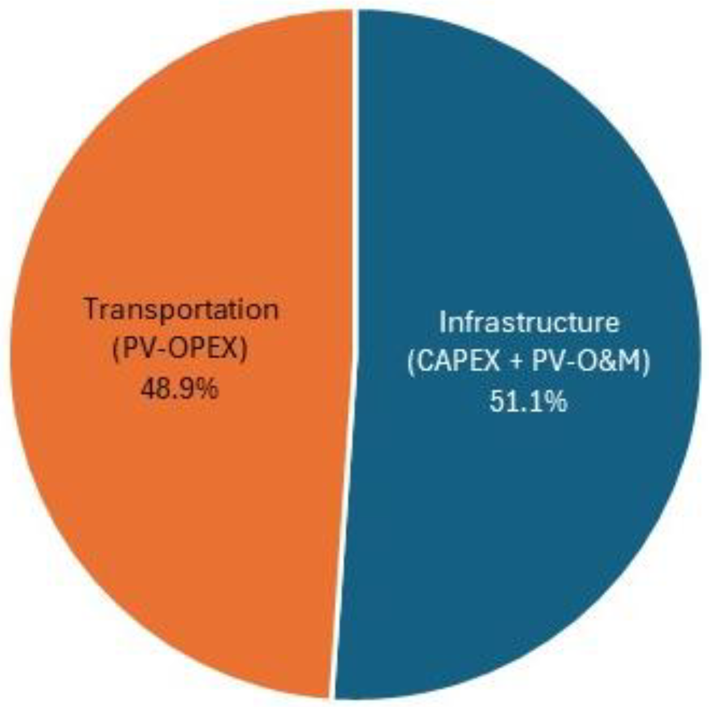
6.5.1. Lifecycle Cost Composition
6.5.2. Infrastructure Cost Breakdown
6.5.3. Levelized Unit Cost
6.6. Sensitivity Analysis
7. Discussion
7.1. Implications for Theory
7.2. Implications for Practice and Policy
7.3. Limitations of the Study and Future Research Directions
8. Conclusions
Author Contributions
Funding
Institutional Review Board Statement
Informed Consent Statement
Data Availability Statement
Acknowledgments
Conflicts of Interest
Abbreviations
| LNG | Liquefied Natural Gas |
| FOB | Free on Board |
| DES | Delivery Ex-Ship |
| MIP | Mixed-integer Programming |
| TSP | Travelling Salesman Problem |
| CRF | Capital Recovery Factor |
Appendix A. Cost Components
Appendix A.1. Transportation Costs
Appendix A.2. Infrastructure CAPEX
Appendix A.2.1. Storage Tank Investment
Appendix A.2.2. Jetty Investment
Appendix A.2.3. Regasification Unit Investment
Appendix A.2.4. Annualised Infrastructure Cost
Appendix A.3. Port Charges and Anchorage Fees
Appendix A.3.1. Upstream Port Charges and Anchorage Fees
Appendix A.3.2. Downstream Port Charges and Anchorage Fees
Appendix B. Geographical Coordinated and Inter-Port Distance Matrix

| Port | Code | Latitude | Longitude |
|---|---|---|---|
| Tangguh | TGU | −2.43967 | 133.13793 |
| Lombok | LOM | −8.58906 | 116.07443 |
| Kupang | KPG | −10.35233 | 123.46157 |
| Maumere | MAU | −8.61989 | 122.33919 |
| Sumbawa | SBW | −8.44416 | 117.33550 |
| Bima | BIM | −8.40697 | 118.69928 |
| Flores | FLO | −8.46073 | 119.94380 |
| Alor | ALO | −8.24389 | 124.53011 |
| Waingapu | WAI | −9.47724 | 120.15198 |
| TGU | LOM | KPG | MAU | SBW | BIM | FLO | ALO | WAI | |
| TGU | - | 1135 | 787 | 781 | 1043 | 959 | 861 | 664 | 920 |
| LOM | 1135 | - | 515 | 414 | 119 | 202 | 269 | 545 | 302 |
| KPG | 787 | 515 | - | 399 | 519 | 590 | 492 | 168 | 206 |
| MAU | 781 | 414 | 399 | - | 322 | 236 | 138 | 177 | 535 |
| SBW | 1043 | 119 | 519 | 322 | - | 136 | 228 | 488 | 367 |
| BIM | 959 | 202 | 590 | 236 | 136 | - | 136 | 367 | 394 |
| FLO | 861 | 269 | 492 | 138 | 228 | 136 | - | 314 | 461 |
| ALO | 664 | 545 | 168 | 177 | 488 | 367 | 314 | - | 275 |
| WAI | 920 | 302 | 206 | 535 | 367 | 394 | 461 | 275 | - |
Appendix C. Detailed Annual LNG Demand Profiles
| (a) | |||||||||||
| Port | Code | Year-1 | Year-2 | Year-3 | Year-4 | Year-5 | Year-6 | Year-7 | Year-8 | Year-9 | Year-10 |
| Lombok | LOM | 1013.70 | 1026.47 | 1039.41 | 1052.50 | 1065.76 | 1079.19 | 1092.79 | 1106.56 | 1120.50 | 1134.62 |
| Kupang | KPG | 141.42 | 143.21 | 145.01 | 146.84 | 148.69 | 150.56 | 152.46 | 154.38 | 156.32 | 158.29 |
| Maumere | MAU | 213.59 | 216.28 | 219.01 | 221.76 | 224.56 | 227.39 | 230.25 | 233.15 | 236.09 | 239.07 |
| Sumbawa | SBW | 1078.60 | 1092.19 | 1105.95 | 1119.89 | 1134.00 | 1148.29 | 1162.75 | 1177.41 | 1192.24 | 1207.26 |
| Bima | BIM | 458.18 | 463.95 | 469.79 | 475.71 | 481.71 | 487.78 | 493.92 | 500.15 | 506.45 | 512.83 |
| Flores | FLO | 106.07 | 107.40 | 108.76 | 110.13 | 111.52 | 112.92 | 114.34 | 115.78 | 117.24 | 118.72 |
| Alor | ALO | 65.38 | 66.21 | 67.04 | 67.89 | 68.74 | 69.61 | 70.49 | 71.37 | 72.27 | 73.18 |
| Waingapu | WAI | 168.55 | 170.67 | 172.82 | 175.00 | 177.20 | 179.44 | 181.70 | 183.99 | 186.30 | 188.65 |
| TOTAL | 3245.49 | 3286.38 | 3327.79 | 3369.72 | 3412.18 | 3455.17 | 3498.71 | 3542.79 | 3587.43 | 3632.63 | |
| (b) | |||||||||||
| Port | Code | Year-11 | Year-12 | Year-13 | Year-14 | Year-15 | Year-16 | Year-17 | Year-18 | Year-19 | Year-20 |
| Lombok | LOM | 1148.92 | 1163.39 | 1178.05 | 1192.90 | 1207.93 | 1223.15 | 1238.56 | 1254.16 | 1269.97 | 1285.97 |
| Kupang | KPG | 160.29 | 162.31 | 164.35 | 166.42 | 168.52 | 170.64 | 172.79 | 174.97 | 177.18 | 179.41 |
| Maumere | MAU | 242.08 | 245.13 | 248.22 | 251.35 | 254.51 | 257.72 | 260.97 | 264.26 | 267.58 | 270.96 |
| Sumbawa | SBW | 1222.47 | 1237.88 | 1253.47 | 1269.27 | 1285.26 | 1301.46 | 1317.85 | 1334.46 | 1351.27 | 1368.30 |
| Bima | BIM | 519.29 | 525.83 | 532.46 | 539.17 | 545.96 | 552.84 | 559.81 | 566.86 | 574.00 | 581.24 |
| Flores | FLO | 120.22 | 121.73 | 123.26 | 124.82 | 126.39 | 127.98 | 129.60 | 131.23 | 132.88 | 134.56 |
| Alor | ALO | 74.11 | 75.04 | 75.99 | 76.94 | 77.91 | 78.89 | 79.89 | 80.89 | 81.91 | 82.95 |
| Waingapu | WAI | 191.03 | 193.44 | 195.87 | 198.34 | 200.84 | 203.37 | 205.93 | 208.53 | 211.16 | 213.82 |
| TOTAL | 3678.40 | 3724.75 | 3771.68 | 3819.20 | 3867.33 | 3916.06 | 3965.40 | 4015.36 | 4065.95 | 4117.19 | |
Appendix D. Bathymetric Data
| Port | 3 m | 6 m | 9 m | 12 m | 15 m | >15 m |
|---|---|---|---|---|---|---|
| LOM | 258.69 | 497.18 | 851.85 | 851.85 | 851.85 | 851.85 |
| KPG | 311.47 | 479.45 | 619.23 | 771.42 | 771.42 | 771.42 |
| MAU | 56.09 | 108.64 | 382.60 | 829.08 | 829.08 | 829.08 |
| SBW | 152.08 | 220.53 | 220.53 | 268.50 | 568.50 | 301.25 |
| BIM | 111.10 | 176.64 | 190.52 | 190.52 | 202.48 | 202.48 |
| FLO | 836.51 | 1089.05 | 1089.05 | 1089.05 | 1089.05 | 1089.05 |
| ALO | 65.00 | 125.00 | 125.00 | 180.10 | 180.10 | 201.48 |
| WAI | 70.00 | 122.00 | 122.00 | 122.00 | 122.00 | 122.00 |
Appendix E. Operational Performance Indicators
| Indicator | Year 1 | Year 5 | Year 10 | Year 15 | Year 20 |
|---|---|---|---|---|---|
| Upstream voyages/year | 21 | 22 | 23 | 25 | 26 |
| Cluster 1 voyages/year | 118 | 124 | 132 | 140 | 150 |
| Cluster 2 voyages/year | 66 | 69 | 74 | 78 | 83 |
| Cluster 3 voyages/year | 24 | 26 | 27 | 29 | 31 |
| Indicator | Year 1 | Year 5 | Year 10 | Year 15 | Year 20 |
|---|---|---|---|---|---|
| Upstream vessel (65,000 m3) | 1 | 1 | 1 | 1 | 1 |
| Cluster 1 vessel (3500 m3) | 1 | 1 | 1 | 2 | 2 |
| Cluster 2 vessel (3500 m3) | 1 | 1 | 1 | 2 | 2 |
| Cluster 3 vessel (10,000 m3) | 1 | 1 | 1 | 1 | 1 |
| Indicator | Year 1 | Year 5 | Year 10 | Year 15 | Year 20 |
|---|---|---|---|---|---|
| Upstream | 47.09% | 49.51% | 52.71% | 56.12% | 59.74% |
| Cluster 1 | 87.01% | 91.48% | 97.39% | 51.84% | 55.19% |
| Cluster 2 | 83.82% | 89.27% | 93.82% | 50.59% | 53.86% |
| Cluster 3 | 62.86% | 66.08% | 70.35% | 74.90% | 79.74% |
| Indicator | Year 1 | Year 5 | Year 10 | Year 15 | Year 20 |
|---|---|---|---|---|---|
| Upstream vessel (65,000 m3) | |||||
| Loading time at source | 0.79 | 0.79 | 0.80 | 0.80 | 0.80 |
| Discharging time at the hub | 1.09 | 1.09 | 1.10 | 1.10 | 1.10 |
| Cluster 1 vessel (3500 m3) | |||||
| Loading time at the hub | 0.69 | 0.69 | 0.69 | 0.69 | 0.69 |
| Discharging time at LOM | 0.76 | 0.76 | 0.76 | 0.76 | 0.76 |
| Cluster 2 vessel (3500 m3) | |||||
| Loading time at the hub | 0.69 | 0.69 | 0.69 | 0.69 | 0.69 |
| Discharging time at BIM | 0.73 | 0.73 | 0.73 | 0.73 | 0.73 |
| Discharging time at FLO | 0.65 | 0.65 | 0.65 | 0.65 | 0.65 |
| Cluster 3 vessel (10,000 m3) | |||||
| Loading time at the hub | 0.81 | 0.81 | 0.81 | 0.81 | 0.81 |
| Discharging time at MAU | 0.69 | 0.69 | 0.69 | 0.69 | 0.69 |
| Discharging time at ALO | 0.65 | 0.65 | 0.65 | 0.65 | 0.65 |
| Discharging time at KPG | 0.67 | 0.67 | 0.67 | 0.67 | 0.67 |
| Discharging time at WAI | 0.68 | 0.68 | 0.68 | 0.68 | 0.68 |
| Indicator | Year 1 | Year 5 | Year 10 | Year 15 | Year 20 |
|---|---|---|---|---|---|
| Storage turnover Upstream | 17.38 | 16.59 | 15.87 | 14.60 | 14.04 |
| Storage turnover Cluster 1 | 3.09 | 2.94 | 2.77 | 2.61 | 2.43 |
| Storage turnover Cluster 2 | 5.53 | 5.29 | 4.93 | 4.68 | 4.40 |
| Storage turnover Cluster 3 | 15.21 | 14.04 | 13.52 | 12.59 | 11.77 |
Appendix F. Genetic Algorithm Convergence Robustness
| Run | Hub | Cluster 1 | Cluster 2 | Cluster 3 | Unit Cost | ||||
|---|---|---|---|---|---|---|---|---|---|
| Port | Vessel | Port | Vessel | Port | Vessel | Port | Vessel | ||
| 1 | SUM | 65,000 | LOM; BIM | 7500 | FLO; ALO; WAI | 3500 | MAU; KPG | 3500 | 5.00 |
| 2 | SUM | 65,000 | LOM; BIM | 7500 | FLO; MAU; WAI | 3500 | WAI; KPG | 3500 | 4.93 |
| 3 | SUM | 65,000 | LOM | 3500 | BIM; FLO | 3500 | MAU; ALO; KPG; WAI | 10,000 | 4.66 |
| 4 | SUM | 65,000 | LOM; BIM | 10,000 | FLO; ALO; WAI | 5000 | MAU; KPG | 5000 | 4.80 |
| 5 | SUM | 65,000 | LOM; BIM | 10,000 | FLO; ALO; WAI | 5000 | MAU; KPG | 3500 | 4.83 |
| 6 | SUM | 65,000 | LOM; BIM | 10,000 | FLO; MAU; ALO | 5000 | WAI; KPG | 3500 | 4.73 |
| 7 | SUM | 65,000 | LOM; BIM | 10,000 | FLO; ALO; WAI | 5000 | MAU; KPG | 3500 | 4.83 |
| 8 | SUM | 65,000 | LOM; BIM | 10,000 | FLO; MAU; ALO | 5000 | WAI; KPG | 3500 | 4.73 |
| 9 | SUM | 65,000 | LOM; BIM | 10,000 | FLO; ALO; WAI | 5000 | MAU; KPG | 5000 | 4.80 |
| 10 | SUM | 65,000 | LOM | 3500 | BIM; FLO | 3500 | MAU; ALO; KPG; WAI | 10,000 | 4.66 |
| 11 | SUM | 65,000 | LOM; BIM | 10,000 | FLO; MAU; ALO | 5000 | WAI; KPG | 3500 | 4.73 |
| 12 | SUM | 65,000 | LOM | 3500 | BIM; FLO | 3500 | MAU; ALO; KPG; WAI | 10,000 | 4.66 |
| 13 | SUM | 65,000 | LOM | 3500 | BIM; FLO | 3500 | MAU; ALO; KPG; WAI | 10,000 | 4.66 |
| 14 | SUM | 65,000 | LOM | 3500 | BIM; FLO | 3500 | MAU; ALO; KPG; WAI | 10,000 | 4.66 |
| 15 | SUM | 65,000 | LOM; BIM | 10,000 | FLO; MAU; ALO | 5000 | WAI; KPG | 3500 | 4.73 |
| 16 | SUM | 65,000 | LOM | 3500 | BIM; FLO | 3500 | MAU; ALO; KPG; WAI | 10,000 | 4.66 |
| 17 | SUM | 65,000 | LOM | 3500 | BIM; FLO | 3500 | MAU; ALO; KPG; WAI | 10,000 | 4.66 |
| 18 | SUM | 65,000 | LOM | 3500 | BIM; FLO | 3500 | MAU; ALO; KPG; WAI | 10,000 | 4.66 |
| 19 | SUM | 65,000 | LOM; BIM | 7500 | FLO; ALO; WAI | 5000 | MAU; KPG | 3500 | 4.95 |
| 20 | SUM | 65,000 | LOM | 3500 | BIM; FLO | 3500 | MAU; ALO; KPG; WAI | 10,000 | 4.66 |
References
- Fauzi, I.; Ispandiari, A.R. Green LNG Supply Chain: Optimizing Distribution in Eastern Indonesia. Evergreen 2024, 11, 2624–2637. [Google Scholar] [CrossRef] [Scilit]
- Yuan, J.; Shi, X.; He, J. LNG market liberalization and LNG transportation: Evaluation based on fleet size and composition model. Appl. Energy 2024, 358, 122657. [Google Scholar] [CrossRef] [Scilit]
- Turan, M.O.; Flamand, T. Optimizing investment and transportation decisions for the European natural gas supply chain. Appl. Energy 2023, 337, 120859. [Google Scholar] [CrossRef] [Scilit]
- Dong, K.; Li, J.; Zhang, H. LNG point supply of villages and towns in China: Challenges and countermeasures. Appl. Energy 2023, 334, 120741. [Google Scholar] [CrossRef] [Scilit]
- Rahmanta, M.A.; Asih, A.M.S.; Sopha, B.M.; Sulancana, B.; Wibowo, P.A.; Hariyostanto, E.; Septiangga, I.J.; Saputra, B.T.A. Insights into small-scale LNG supply chains for cost-efficient power generation in Indonesia. Energies 2025, 18, 2709. [Google Scholar] [CrossRef] [Scilit]
- El Ghazi, F.; Lechheb, C.; Kaitouni, O.D. Midstream supply chain infrastructure facilities and optimization opportunities for emerging LNG markets. Int. J. Energy Econ. Policy 2023, 13, 175–186. [Google Scholar] [CrossRef] [Scilit]
- Mei, Q.; Qinyou, H.; Hu, Y.; Yang, Y.; Liu, X.; Huang, Z.; Wang, P. Structural analysis and vulnerability assessment of the European LNG maritime supply chain network (2018–2020). Ocean Coast. Manag. 2024, 253, 107126. [Google Scholar] [CrossRef] [Scilit]
- Khalilpour, R.; Karimi, I.A. Selection of liquefied natural gas (LNG) contracts for minimizing procurement cost. Ind. Eng. Chem. Res. 2011, 50, 10298–10312. [Google Scholar] [CrossRef] [Scilit]
- International Gas Union (IGU). World LNG Report 2024. Available online: https://www.igu.org (accessed on 15 January 2026).
- GIIGNL. The LNG Industri—Annual Report 2024. Available online: https://giignl.org (accessed on 15 January 2026).
- Sharples, J. LNG Contracts in the Context of Market Turbulence and an Uncertain Future; Oxford Institute for Energy Studies: Oxford, UK, 2023. [Google Scholar]
- Talus, K.; Steck, G.; Atkin, J. EU methane regulation and its impact on LNG imports. J. World Energy Law Bus. 2025, 18, jwae022. [Google Scholar] [CrossRef] [Scilit]
- Hadi, F.; Supomo, H.; Achmadi, T.; Baihaqi, I. An optimization model for designing the LNG supply chain and required infrastructure. Int. Rev. Model. Simul. 2025, 18, 373. [Google Scholar] [CrossRef] [Scilit]
- Purwosaputra, A.A.; Artana, K.B.; Dinariyana, A.A.B. A state of the art of the LNG supply chain models: A quest for an optimum model fitting inter-islands distribution in an archipelago country. Int. Rev. Mech. Eng. 2022, 16, 204–248. [Google Scholar] [CrossRef] [Scilit]
- Machfudiyanto, R.A.; Muslim, F.; Humang, W.P.; Wahjuningsih, N.; Kamil, I.; Ichsan, M.; Putra, Y.Y.A. Optimization of the risk-based small-scale LNG supply chain in the Indonesian archipelago. Heliyon 2023, 9, e19047. [Google Scholar] [CrossRef] [Scilit] [PubMed]
- Jokinen, R.; Petterson, F.; Saxén, H. An MILP model for optimization of a small-scale LNG supply chain along a coastline. Appl. Energy 2015, 138, 423–431. [Google Scholar] [CrossRef] [Scilit]
- Bittante, A.; Petterson, F.; Saxén, H. Optimization of a small-scale LNG supply chain. Energy 2018, 148, 79–89. [Google Scholar] [CrossRef] [Scilit]
- Bittante, A.; Saxén, H. Design of small LNG supply chain by multi-period optimization. Energies 2020, 13, 6704. [Google Scholar] [CrossRef] [Scilit]
- Muzhoffar, D.A.F.; Auzani, A.S. Comparative analysis of LNG distribution schemes using milk-run and hub-and-spoke methods in Eastern Indonesia. J. Sains Teknol. Transp. Marit. 2024, 6, 36–44. [Google Scholar]
- Antara, D.S.; Artana, K.B.; Dinariyana, A.A.B.; Adhita, I.G.M.S. Enhancing sustainable energy supply: Clustering analysis of LNG distribution for Indonesian power plants using K-means method. Int. Rev. Mech. Eng. 2024, 18, 590–597. [Google Scholar] [CrossRef] [Scilit]
- Machfudiyanto, R.A.; Humang, W.P.; Kamil, I.; Latief, Y.; Wahjuningsih, N.; Putra, Y.Y.A. Enhancing small-scale LNG supply chains: Risk mitigation strategies for archipelagic distribution. Clean. Logist. Supply Chain 2025, 16, 100249. [Google Scholar] [CrossRef] [Scilit]
- Zhang, H.; Wu, Y.; Zhen, L.; Jin, Y.; Wang, S. Optimization problems in liquefied natural gas transport and storage for multimodal transport companies. Electron. Res. Arch. 2024, 32, 4828–4844. [Google Scholar] [CrossRef] [Scilit]
- Siahaan, J.J.A.; Pratiwi, E.; Setyorini, P.D. Study of Green-Ship Routing Problem (G-VRP) Optimization for Indonesia LNG Distribution. IOP Conf. Ser. Earth Environ. Sci. 2020, 557, 012018. [Google Scholar] [CrossRef] [Scilit]
- Pratama, Y.W.; Reyseliani, N.; Purwanto, W.W. An MILP framework for gas supply chain infrastructure planning with endogenous logistics schemes. J. Nat. Gas Sci. Eng. 2025, 143, 205742. [Google Scholar] [CrossRef] [Scilit]
- Yu, H.; Wu, W.; Zhang, X.; Fang, Z.; Fu, X.; Xu, L.; Liu, J. Optimization-based global liquefied natural gas shipping network management for emission reduction. Ocean Eng. 2025, 321, 120366. [Google Scholar] [CrossRef] [Scilit]
- Wu, X.; Wang, D.; Wen, L.; Xiao, Y.; Wu, C.; Wu, Y.; Zhou, Y. Neural Combinatorial Optimization Algorithms for Solving Vehicle Routing Problems: A Comprehensive Survey with Perspectives. arXiv 2025. [Google Scholar] [CrossRef] [Scilit]
- Simchi-Levi, D.; Mellou, K.; Menache, I.; Pathuri, J. Large Language Models for Supply Chain Decisions. Available online: https://ssrn.com/abstract=5370043 (accessed on 29 June 2025). [CrossRef] [Scilit]
- Wang, Y.; Liang, X. Application of Reinforcement Learning Methods Combining Graph Neural Networks and Self-Attention Mechanisms in Supply Chain Route Optimization. Sensors 2025, 25, 955. [Google Scholar] [CrossRef] [Scilit]
- Dobrota, Đ.; Lalić, B.; Komar, I. Problem of Boil—Off in LNG Supply Chain. Trans. Marit. Sci. 2013, 2, 91–100. [Google Scholar] [CrossRef] [Scilit]
- Eriksen, U.; Kristiansen, J.; Fagerholt, K.; Pantuso, G. Planning a maritime supply chain for liquefied natural gas under uncertainty. Marit. Transp. Res. 2022, 3, 100061. [Google Scholar] [CrossRef] [Scilit]
- Goldberg, D.E. Genetic Algorithms in Search, Optimization and Machine Learning; Addison-Wesley Longman Publishing Co., Inc.: Boston, UK, 1989. [Google Scholar]
- Eiben, A.E.; Hinterding, R.; Michalewicz, Z. Parameter control in evolutionary algorithms. IEEE Trans. Evol. Comput. 1999, 3, 124–141. [Google Scholar] [CrossRef] [Scilit]
- Shin, Y.; Lee, Y.P. Design of a boil-off natural gas reliquefaction control system for LNG carriers. Appl. Energy 2009, 86, 37–44. [Google Scholar] [CrossRef] [Scilit]
- Duan, Z.; Xue, H.; Gong, X.; Tang, W. A thermal non-equilibrium model for predicting LNG boil-off in storage tanks incorporating the natural convection effect. Energy 2021, 233, 121162. [Google Scholar] [CrossRef] [Scilit]
- Keputusan Menteri ESDM No. 13 K/13/MEM/2020 Tentang Penugasan Pelaksanaan Penyediaan Pasokan dan Pembangunan Infrastruktur Liquefied Natural Gas (LNG), Serta Konversi Penggunaan Bahan Bakar Minyak Dengan Liquefied Natual Gas (LNG) Dalam Penyediaan Tenggara Listrik [Decree of the Minister of Energy and Mineral Resources No. 13 K/13/MEM/2020 Concerning the Assignment for the Implementation of Supply Provision and Infrastructure Development for Liquefied Natural Gas, and the Conversion from Fuel Oil to Liquefied Natural Gas in Power Generation]. Available online: https://jdih.esdm.go.id/dokumen/download?id=Kepmen+13+K+2020.pdf (accessed on 22 January 2026).
- Keputusan Menteri ESDM No. 249.K/MG.01/MEM.M/2022 Tentang Penugasan Pelaksanaan Penyediaan Pasokan dan Pembangunan Infrastruktur Liquefied Natural Gas, Serta Konversi Dari Penggunaan Bahan Bakar Minyak Dengan Liquefied Natual Gas Dalam Penyediaan Tenaga Listrik [Decree of the Minister of Energy and Mineral Resources No. 13 K/13/MEM/2020 Concerning the Assignment for the Implementation of Supply Provision and Infrastructure Development for Liquefied Natural Gas, and the Conversion from Fuel Oil to Liquefied Natural Gas in Power Generation]. Available online: https://jdih.esdm.go.id/common/dokumen-external/Kepmen%20ESDM%20No.%20249.K-MG.01-MEM.M-2022.pdf (accessed on 22 January 2026).
- PT. PLN (Persero). Rencana Usaha Penyediaan Tenaga Listrik (RUPTL) 2021–2030 [Electricity Supply Business Plan (RUPTL) 2021–2030]; PT. PLN (Persero): Jakarta, Indonesia, 2021. [Google Scholar]
- De Mone, G. Measuring and Evaluating Port Performance and Productivity; UNCTAD Monographs on Port Management No. 6; United Nations Conference on Trade and Development: Geneva, Switzerland, 1987. [Google Scholar]
- Zain, R.A. Developing Parametric Modelling for Class 4 Estimates of Pier and Jetty Construction by Analysing Historical Databases Using AI Tools and EVM Techniques. Available online: https://www.pertamina.com (accessed on 12 January 2026).


| Related Literature | Contract Scheme | Demand Treatment | Upstream Logistics | Hub-and-Spoke | Infrastructure Endogeneity | Terminal Capacity Constraint | Solution Approach | Real Case Study |
|---|---|---|---|---|---|---|---|---|
| Jokinen et al. [16] | DES | Static | Exogenous | ☑ | ☒ | ☒ | MILP | ☒ |
| Bittante et al. [17] | DES | Static | Exogenous | ☑ | ☒ | ☒ | MILP | ☒ |
| Bittante & Saxén [18] | DES | Multi-period | Exogenous | ☑ | ☒ | ☒ | MILP | ☒ |
| Machfudiyanto et al. [15] | DES | Static | Exogenous | ☑ | ☒ | ☒ | MILP + Risk | ☑ |
| Rahmanta et al. [5] | DES | Static | Exogenous | ☑ | ☒ | ☒ | MILP | ☑ |
| Yuan et al. [2] | FOB | Static | Exogenous | ☒ | ☒ | ☒ | Fleet Optimisation | ☑ |
| Mei et al. [7] | FOB | Static | Exogenous | ☒ | ☒ | ☒ | Network Analysis | ☑ |
| Pratama et al. [24] | DES | Multi-period | Exogenous | ☑ | ☑ (Partial) | ☒ | MILP | |
| This Study | FOB | Time-dependent deterministic | Endogenous | ☑ | ☑ (Fully derived) | ☑ | Two-Stage: MILP + TSP | ☑ |
| Category | Symbol | Description |
|---|---|---|
| Set and Indices | P | Set of destination ports |
| H | Set of candidate hub ports, | |
| K | Set of downstream clusters | |
| T | Set of time periods (years) | |
| V | Set of vessel size classes | |
| i, j | Indices for destination ports | |
| h, k, t, v | Indices for hub, cluster, time, and vessel | |
| Parameters | Total transportation cost in year t | |
| Total infrastructure investment (CAPEX) | ||
| A | Capital recovery factor (CRF) | |
| r | Discount rate | |
| Total regional LNG demand in year t | ||
| Demand at destination port i in year t | ||
| Net cargo capacity of vessel class v for the upstream segment | ||
| Net cargo capacity of vessel class v for cluster k | ||
| Upstream call frequency for vessel v required in year t | ||
| Downstream voyage frequency for vessel v in cluster k in year t | ||
| Maximum allowable vessel call frequency at the source | ||
| Distance between port i and j | ||
| Decision Variables | 1 if port h is selected as hub, 0 otherwise | |
| 1 if port i is assigned to cluster k, 0 otherwise | ||
| 1 if vessel v is assigned to serve hub h (upstream), 0 otherwise | ||
| 1 if vessel v is assigned to serve cluster k (downstream), 0 otherwise | ||
| 1 if vessel travels directly from port i to j, 0 otherwise | ||
| Auxiliary variables | Sequence variable for port visits in the routing sub-problem |
| Port Name | Port Code | Year 1 | Year 5 | Year 10 | Year 15 | Year 20 |
|---|---|---|---|---|---|---|
| Lombok | LOM | 1013.70 | 1065.76 | 1134.62 | 1207.93 | 1285.97 |
| Kupang | KPG | 141.42 | 148.69 | 158.29 | 168.52 | 179.41 |
| Maumere | MAU | 213.59 | 224.56 | 239.07 | 254.51 | 270.96 |
| Sumbawa | SBW | 1078.60 | 1134.00 | 1207.26 | 1285.26 | 1368.30 |
| Bima | BIM | 458.18 | 481.71 | 512.83 | 545.96 | 581.24 |
| Flores | FLO | 106.07 | 111.52 | 118.72 | 126.39 | 134.56 |
| Alor | ALO | 65.38 | 68.74 | 73.18 | 77.91 | 82.95 |
| Waingapu | WAI | 168.55 | 177.20 | 188.65 | 200.84 | 213.82 |
| Total | Region | 3245.49 | 3412.18 | 3632.63 | 3867.33 | 4117.19 |
| Segment | Vessel Class (m3) | Speed (Knots) | Charter Rate (USD/Day) * | Draft (m) | Disch Rate (m3/h) | Fuel Consumption (MT/Day) * | |||
|---|---|---|---|---|---|---|---|---|---|
| Loading | Discharging | Sailing | Idle | ||||||
| Downstream | 3500 | 8.40 | 11,000 | 4.45 | 1000 | 2.14 | 3.42 | 7.62 | 1.46 |
| 5000 | 8.40 | 13,000 | 5.07 | 1000 | 2.52 | 3.93 | 9.09 | 1.71 | |
| 6500 | 8.40 | 16,100 | 5.54 | 2000 | 2.84 | 4.34 | 10.34 | 1.93 | |
| 7500 | 9.10 | 17,000 | 5.81 | 2000 | 3.03 | 4.59 | 11.10 | 2.05 | |
| 10,000 | 9.10 | 20,800 | 6.37 | 2000 | 3.46 | 5.13 | 12.79 | 2.34 | |
| 15,500 | 9.10 | 27,100 | 7.30 | 5100 | 4.25 | 6.07 | 15.87 | 2.85 | |
| 18,500 | 9.10 | 29,500 | 7.71 | 5100 | 4.59 | 6.50 | 17.32 | 3.09 | |
| 20,000 | 9.10 | 30,500 | 7.89 | 5100 | 4.79 | 6.70 | 18.00 | 3.20 | |
| Upstream | 30,000 | 10.50 | 39,400 | 8.91 | 5100 | 5.73 | 7.83 | 21.98 | 3.84 |
| 45,000 | 11.00 | 49,900 | 10.06 | 5100 | 6.90 | 9.16 | 26.84 | 4.61 | |
| 65,000 | 13.00 | 63,700 | 11.21 | 5100 | 8.17 | 10.56 | 32.18 | 5.45 | |
| 125,000 | 14.00 | 94,600 | 13.58 | 5100 | 11.03 | 13.58 | 44.42 | 7.32 | |
| 135,000 | 14.50 | 98,800 | 13.89 | 5100 | 11.43 | 13.99 | 46.14 | 7.58 | |
| 145,000 | 14.50 | 102,900 | 14.18 | 5100 | 11.81 | 14.38 | 47.79 | 7.83 | |
| Category | Parameter/Component | Value/Formula | Unit/Note |
|---|---|---|---|
| Storage Facility | Hub port (Flat-Bottom tank) | 1000 | USD/m3 |
| Spoke ports (Bullet tank) | 2,420,000 | USD/unit (1000 m3) | |
| Heel (unpumpable) | 10 | % of capacity | |
| Safety Buffer | 3 | Days of daily demand | |
| Marine Infrastructure | Jetty CAPEX | See Appendix A.2 | Function of vessel size |
| Trestle CAPEX | Function of length | Driven by bathymetry | |
| Regasification | Regas Unit CAPEX | See Appendix A.2 | Function of peak load |
| Peak load factor | 135 | % of daily demand | |
| Operational | Infrastructure O&M | 5 | % of total CAPEX/year |
| Annual operating days | 355 | Days/year |
| Parameter | Symbol | Value | Unit |
|---|---|---|---|
| Planning Horizon | T | 20 | Years |
| Discount Rate (WACC) | r | 9.5 | % |
| Annual Inflation Rate | i | 2 | % |
| Operating Days | 355 | Days/year |
| Segment | Cluster | Vessel Class (m3) | Fleet Size (Unit) | Annual Freq. [Min]–[Max] | Fleet Utilisation [Min]–[Max] |
|---|---|---|---|---|---|
| Upstream | TGU ⟶ SBW | 65,000 | Year 1–20 (1 unit) | 21–26 | 47.09–59.74% |
| Downstream | Cluster 1 | 3500 | Year 1–12 (1 unit) Year 13–20 (2 units) | 118–150 | 50.56–99.86% |
| Cluster 2 | 3500 | Year 1–14 (1 unit) Year 15–20 (2 units) | 66–83 | 50.59–99.92% | |
| Cluster 3 | 10,000 | Year 1–20 (1 unit) | 24–31 | 62.86–79.74% |
| Segment/Cluster | Optimal Port Sequence | Round-Trip Distance (nm) |
|---|---|---|
| Upstream | TGU ⟶ SBW ⟶ TGU | 2086 |
| Cluster 1 | SBW ⟶ LOM ⟶ SBW | 238 |
| Cluster 2 | SBW ⟶ BIM ⟶ FLO ⟶ SBW | 500 |
| Cluster 3 | SBW ⟶ MAU ⟶ ALO ⟶ KPG ⟶ WAI ⟶ SBW | 1240 |
| Port | Role | Storage | Trestle Length (m) | BOR * [Min]–[Max] | Regas (m3/Day) | |
|---|---|---|---|---|---|---|
| Capacity (m3) | Type | |||||
| Sumbawa | Hub | 76,000 | Flat-Bottom tank | 270 | 46.38–58.75% | 1847.20 |
| Lombok | Spoke | 8000 | Bullet tank | 500 | 24.43–31.04% | 1736.06 |
| Bima | Spoke | 5000 | Bullet tank | 180 | 13.21–16.63% | 784.67 |
| Flores | Spoke | 2000 | Bullet tank | 1090 | 11.74–14.77% | 181.65 |
| Alor | Spoke | 2000 | Bullet tank | 130 | 4.25–5.48% | 111.98 |
| Waingapu | Spoke | 4000 | Bullet tank | 130 | 4.46–5.75% | 288.65 |
| Maumere | Spoke | 5000 | Bullet tank | 390 | 4.55–5.87% | 365.79 |
| Kupang | Spoke | 3000 | Bullet tank | 780 | 4.46–5.75% | 242.20 |
| Port/Cluster | Storage (USD) | Jetty + Trestle (USD) | Regas (USD) | Total CAPEX (USD) | Share (%) |
|---|---|---|---|---|---|
| Hub (SBW) | 76,000,000 | 6,648,251 | 31,392,456 | 114,040,707 | 34.1% |
| Cluster 1 | 19,360,000 | 5,337,742 | 38,148,822 | 62,846,564 | 18.8% |
| LOM | 19,360,000 | 5,337,742 | 38,148,822 | 62,846,564 | |
| Cluster 2 | 16,940,000 | 11,806,028 | 26,947,489 | 55,693,517 | 16.7% |
| BIM | 12,100,000 | 3,997,838 | 14,842,511 | 30,940,349 | |
| FLO | 4,840,000 | 7,808,190 | 12,104,977 | 24,753,167 | |
| Cluster 3 | 33,880,000 | 21,930,999 | 45,557,170 | 101,368,169 | 30.4% |
| MAU | 12,100,000 | 5,618,834 | 12,660,380 | 30,379,214 | |
| ALO | 4,840,000 | 4,530,162 | 7,744,715 | 17,114,877 | |
| KPG | 7,260,000 | 7,251,842 | 13,224,820 | 27,736,661 | |
| WAI | 9,680,000 | 4,530,162 | 11,927,256 | 26,137,418 | |
| TOTAL | 146,180,000 | 45,723,020 | 142,045,937 | 333,948,957 | 100% |
| Scenario | Ports | Vessel Class (m3) | Unit Cost (USD/MMBtu) |
|---|---|---|---|
| Base-case | Hub (SBW) | 65,000 | 4.66 |
| Cluster 1 (LOM) | 3500 | ||
| Cluster 2 (BIM, FLO) | 3500 | ||
| Cluster 3 (MAU, ALO, KPG, WAI) | 10,000 | ||
| Demand −20% | Hub (SBW) | 65,000 | 5.35 |
| Cluster 1 (LOM) | 3500 | ||
| Cluster 2 (BIM, FLO) | 3500 | ||
| Cluster 3 (MAU, ALO, KPG, WAI) | 7500 | ||
| Demand −10% | Hub (SBW) | 65,000 | 4.97 |
| Cluster 1 (LOM) | 3500 | ||
| Cluster 2 (BIM, FLO) | 3500 | ||
| Cluster 3 (MAU, ALO, KPG, WAI) | 10,000 | ||
| Demand +10% | Hub (SBW) | 125,000 | 5.31 |
| Cluster 1 (LOM) | 3.500 | ||
| Cluster 2 (BIM, FLO) | 5000 | ||
| Cluster 3 (MAU, ALO, KPG, WAI) | 10,000 | ||
| Demand +20% | Hub (SBW) | 125,000 | 5.02 |
| Cluster 1 (LOM) | 5000 | ||
| Cluster 2 (BIM, FLO) | 5000 | ||
| Cluster 3 (MAU, ALO, KPG, WAI) | 10,000 |
Disclaimer/Publisher’s Note: The statements, opinions and data contained in all publications are solely those of the individual author(s) and contributor(s) and not of MDPI and/or the editor(s). MDPI and/or the editor(s) disclaim responsibility for any injury to people or property resulting from any ideas, methods, instructions or products referred to in the content. |
© 2026 by the authors. Licensee MDPI, Basel, Switzerland. This article is an open access article distributed under the terms and conditions of the Creative Commons Attribution (CC BY) license.
Share and Cite
Hadi, F.; Supomo, H.; Achmadi, T.; Baihaqi, I. An Integrated Optimisation Model for LNG Supply Chain Planning and Infrastructure Under FOB Scheme with Time-Dependent Demand. Logistics 2026, 10, 61. https://doi.org/10.3390/logistics10030061
Hadi F, Supomo H, Achmadi T, Baihaqi I. An Integrated Optimisation Model for LNG Supply Chain Planning and Infrastructure Under FOB Scheme with Time-Dependent Demand. Logistics. 2026; 10(3):61. https://doi.org/10.3390/logistics10030061
Chicago/Turabian StyleHadi, Firmanto, Heri Supomo, Tri Achmadi, and Imam Baihaqi. 2026. "An Integrated Optimisation Model for LNG Supply Chain Planning and Infrastructure Under FOB Scheme with Time-Dependent Demand" Logistics 10, no. 3: 61. https://doi.org/10.3390/logistics10030061
APA StyleHadi, F., Supomo, H., Achmadi, T., & Baihaqi, I. (2026). An Integrated Optimisation Model for LNG Supply Chain Planning and Infrastructure Under FOB Scheme with Time-Dependent Demand. Logistics, 10(3), 61. https://doi.org/10.3390/logistics10030061