Use of Modern Regression Analysis in the Dielectric Properties of Foods


Abstract
1. Introduction
- Variables including temperature, moisture content, and frequencywhere is the dielectric constant or the dielectric loss factor, is the temperature in °C, is the moisture content (wet basis, w.b. or dry basic, d.b.) in %, and is the applied frequency in MHz.
- Variables including temperature and moisture content
- Only one variable with other factors fixed
2. Materials and Methods
2.1. Regression Analysis
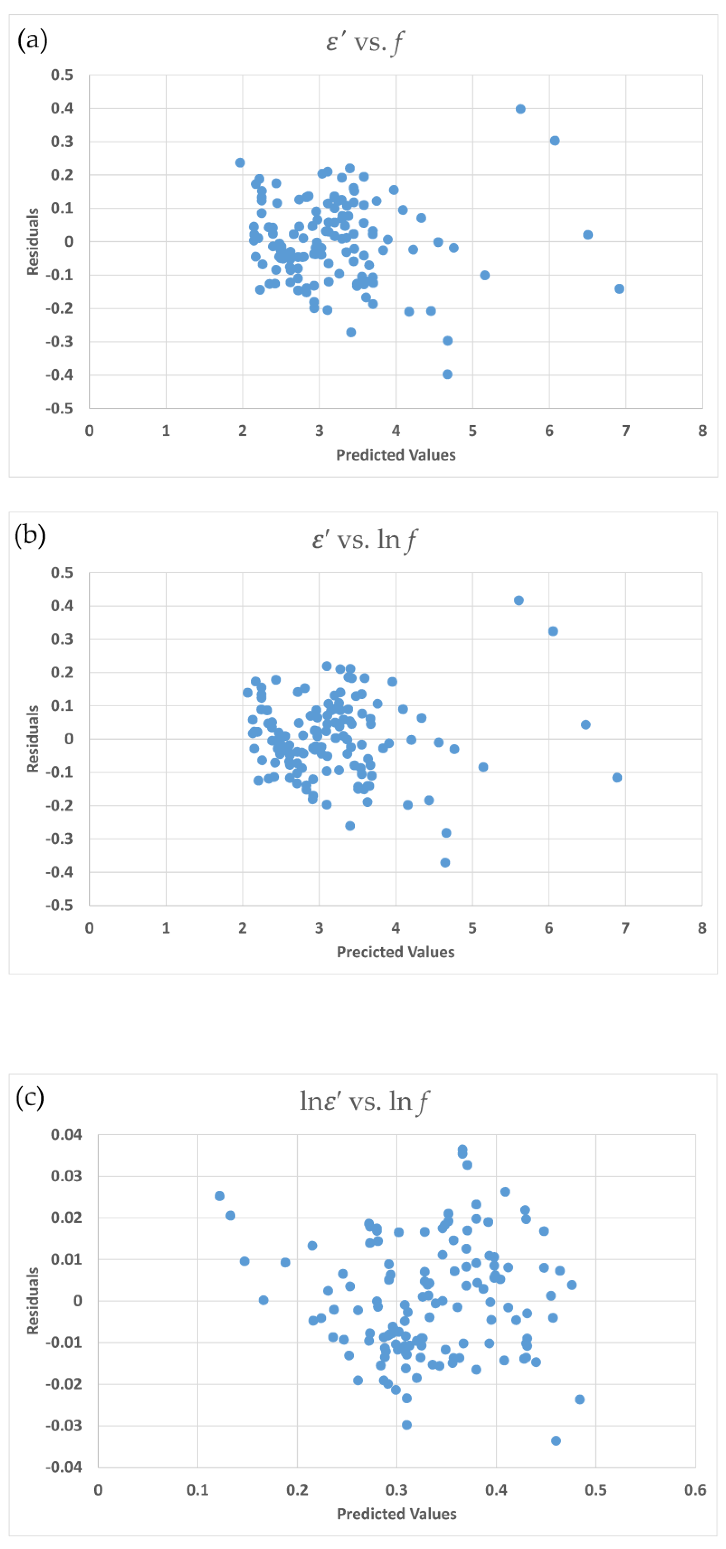
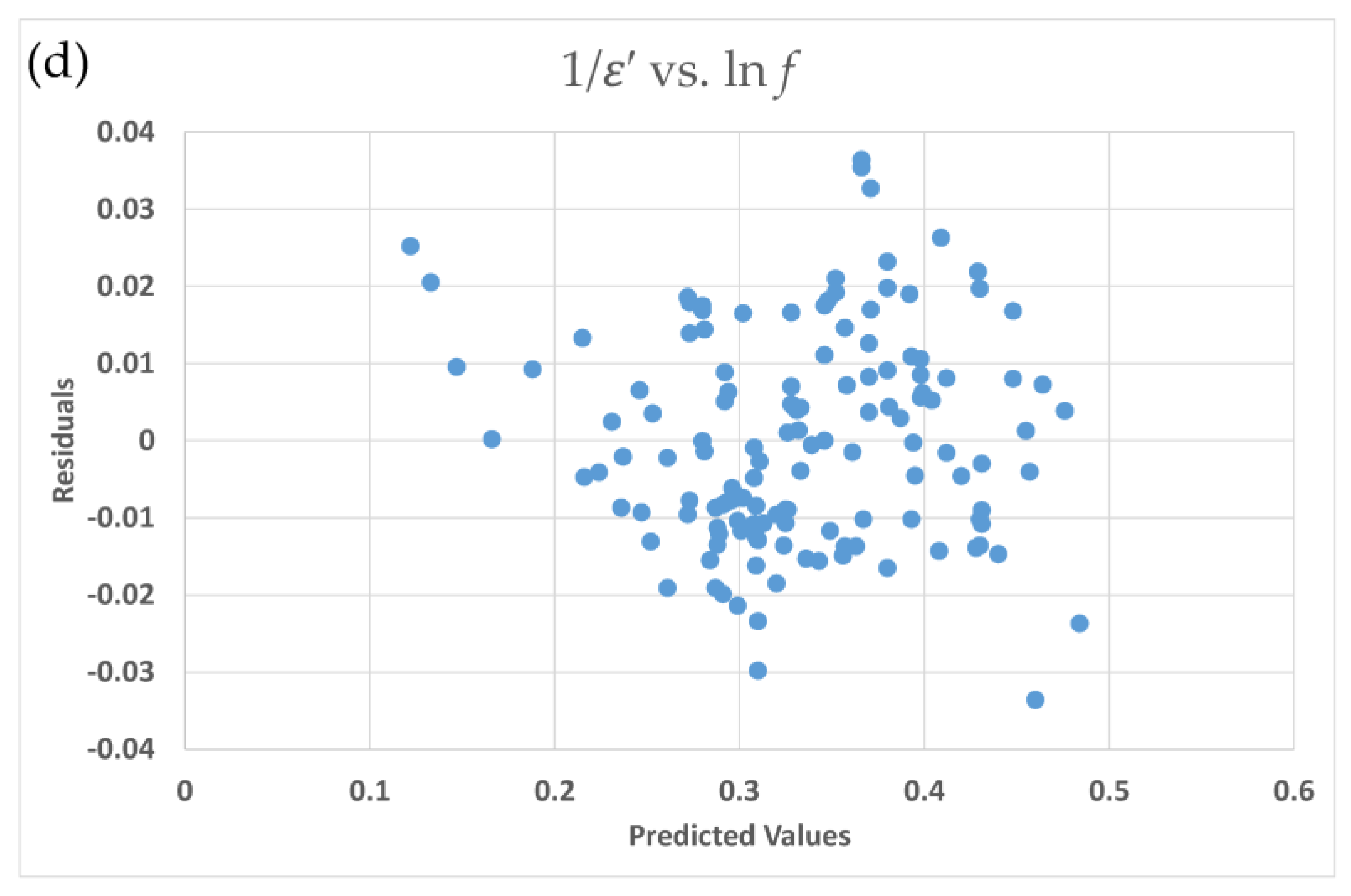
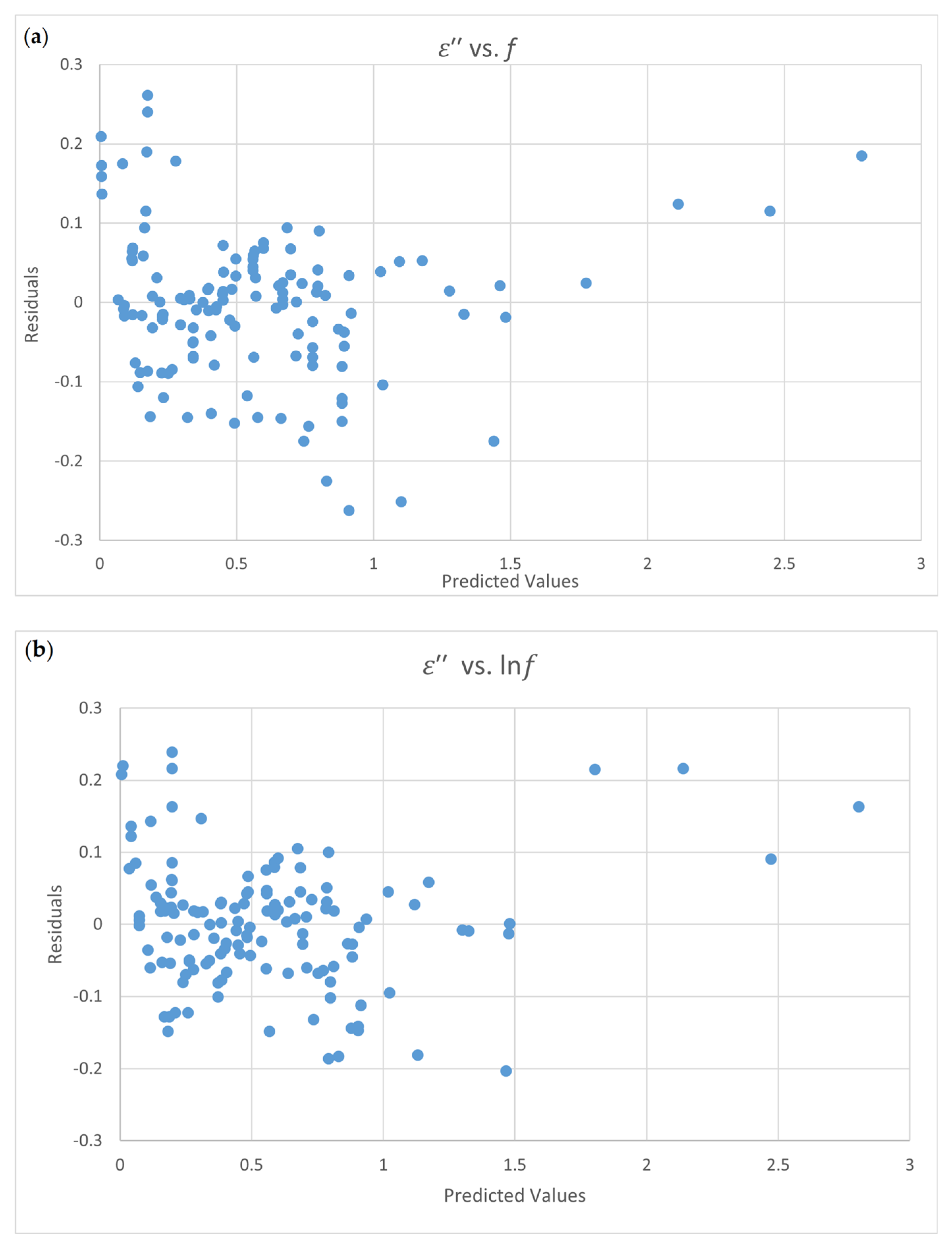
2.1.1. Residual Plots
2.1.2. Normality Test
2.1.3. Constant Variance Test
2.1.4. Transformation
2.2. The Effect of the Storage Time
2.3. Categorical Testing
- Two categories:
- 2.
- Three categories:
- 3.
- Four categories:
2.4. Criterion of the Model Comparison
2.5. Literature Survey
3. Results
3.1. The Dielectric Equations with Three Variables
3.1.1. Egg White Powder
3.1.2. Chicken Flour
(0.0000000260 × f2) + (0.000117 × X2) + (0.000000459 × T × f) + (0.00000309 × T × X)
+ (0.00000239 × f × X) − (0.0000000544 × T × f × X)
ln f2) + (0.00903 × X2) + (0.00888 × T × ln f) + (0.0122 × T × X) − (0.000623 × T × ln f × X)
− (0.0000115 × T3) − (0.00000589 × (T × f) 2) − (0.00000191 × (T × X)2).
3.1.3. Bread
(0.000194 × T × ln f) + (0.000307 × T × X).
ln f2) − (0.00369 × T × ln f) − (0.00291 × T × X) − (0.0137 × ln f × X)
3.1.4. Black-Eyed Peas
3.1.5. Macadamia Nut Kernels
3.2. Equation for Dielectric Properties with Two Variables
3.2.1. Liquid and Precooked Egg White
(0.00155 × T × ln f)
ln f2) + (0.0000193 × T × ln f)
(0.00113 × T × ln f)
(0.00140 × T × ln f)
− (0.0000852 × T × ln f)
3.2.2. Fruits, Nuts, and Insects
3.3. Effect of the Storage Time on the Dielectric Properties of Eggs
3.4. Categorical Test of Two Factors
3.4.1. Butter
× T2 × z) − (0.0680 × ln f) − (0.349 × ln f × z)
× T2 × z) − (0.192 × ln f) − (2.600 × ln f × z)
3.4.2. Salmon Fish
3.5. Categorical Test of Three Factors
3.6. Categorical Test of Four Factors
3.6.1. Salmon Fillets
3.6.2. Pecan Kernels
3.7. The Best Regression Equations for Each Food Ingredient
3.7.1. Egg White Powder
ln f2) + (0.00180 × X2) + (0.00181 × T × ln f+ (0.00159 × T × X) − (0.00422 × ln f × X) −
(0.000197 × T × ln f × X)
(0.00729 × T × X) + (0.0236 × ln f × X) − (0.000924 × T × ln f × X)
3.7.2. Chicken Flour
× f2) + (0.000117 × X2) + (0.000000459 × T × f) + (0.00000309 × T × X) + (0.00000239 × f × X) −
(0.0000000544 × T × f × X)
(0.00903 × X2) + (0.00888 × T × ln f) + (0.0122 × T × X) − (0.000623 × T × ln f × X) − (0.0000115 ×
T3) − (0.00000589 × (T × f) 2) − (0.00000191 × (T × X)2)
3.7.3. Bread
ln f) + (0.000307 × T × X)
(0.00369 × T × ln f) − (0.00291 × T × X) − (0.0137 × ln f × X)
3.7.4. Black-Eyed Peas
+ (0.00926 × X2) + (0.000677 × T × ln f) + (0.000693 × T × X) − (0.00662 × ln f × X) − (0.0000247
× T × ln f × X) − (0.00000124 × (T × X)2)
(0.0131 × X2) + (0.00674 × T × ln f) + (0.00315 × T × X) + (0.0161 × ln f × X) − (0.0000621 × T ×
ln f × X) − (0.00000770 × T × ln f2) − (0.000000970 × (T × X)2)
3.7.5. Macadamia Nut Kernels
+ (0.00000963 × X2) − (0.000227 × T × ln f) + (0.000304 × T × X) − (0.00904 × ln f × X) −
(0.00000325 × T × ln f × X) − (0.000000205 × T × ln f2) − (0.0000000679 × (T × X)2)
− (0.00381 × X2) − (0.00102 × T × ln f) + (0.000778 × T × X) − (0.0397 × ln f) × X) − (0.000118 × T
× ln f × X) + (0.000000144 × (T × X)2)
3.7.6. Liquid Egg White
3.7.7. Precooked Egg White
(0.0000852 × T × ln f)
3.7.8. Almond
3.7.9. Walnut
4. Discussion
5. Conclusions
Supplementary Materials
Author Contributions
Funding
Conflicts of Interest
References
- Icier, F.; Baysal, T. Dielectrical properties of food materials—1: Factors affecting and industrial uses. Crit. Rev. Food Sci. Nutr. 2004, 44, 465–471. [Google Scholar] [CrossRef] [PubMed]
- Icier, F.; Baysal, T. Dielectrical properties of food materials—2: Measurement techniques. Crit. Rev. Food Sci. Nutr. 2004, 44, 473–478. [Google Scholar] [CrossRef] [PubMed]
- Venkatesh, M.S.; Raghavan, G.S.V. An overview of dielectric properties measuring techniques. Can. Biosyst. Eng. 2005, 47, 15–30. [Google Scholar]
- Jha, S.N.; Narsaiah, K.; Basediya, A.L.; Sharma, R.; Jaiswal, P.; Kumar, R.; Bhardwaj, R. Measurement techniques and application of electrical properties for nondestructive quality evaluation of foods—A review. J. Food Sci. Technol. 2011, 48, 387–411. [Google Scholar] [CrossRef] [PubMed]
- Sosa-Morales, M.E.; Valerio-Junco, L.; López-Malo, A.; García, H.S. Dielectric properties of foods: Reported data in the 21st century and their potential applications. LWT Food Sci. Technol. 2010, 43, 1169–1179. [Google Scholar] [CrossRef]
- Khaled, D.E.; Novas, N.; Gazquez, J.A.; Garcia, R.M.; Manzano-Agugliaro, F. Fruit and vegetable quality assessment via dielectric sensing. Sensors 2015, 15, 15363–15397. [Google Scholar] [CrossRef]
- Venkatesh, M.S.; Raghavan, G.S.V. An overview of microwave processing and dielectric properties of agri-food materials. Biosyst. Eng. 2004, 88, 1–18. [Google Scholar] [CrossRef]
- Boreddy, S.R.; Subbiah, J. Temperature and moisture dependent dielectric properties of egg white powder. J. Food Eng. 2016, 168, 60–67. [Google Scholar] [CrossRef]
- Wang, J.; Tang, J.; Wang, Y.; Swanson, B. Dielectric properties of egg whites and whole eggs as influenced by thermal treatments. LWT Food Sci. Technol. 2009, 42, 1204–1212. [Google Scholar] [CrossRef]
- Guo, W.; Trabelsl, S.; Nelson, S.O.; Jones, D.R. Storage effects on dielectric properties of eggs from 10 to 1800 MHz. J. Food Sci. 2007, 72, 335–340. [Google Scholar] [CrossRef]
- Guo, W.; Tiwari, G.; Tang, J.; Wang, S. Frequency, moisture and temperature-dependent dielectric properties of chickpea flour. Biosyst. Eng. 2008, 101, 217–224. [Google Scholar] [CrossRef]
- Jiao, S.; Johnson, J.A.; Tang, J.; Tiwari, G.; Wang, S. Dielectric properties of cowpea weevil, black-eyed peas and mung beans with respect to the development of radio frequency heat treatments. Biosyst. Eng. 2011, 108, 280–291. [Google Scholar] [CrossRef]
- Ahmed, J.; Ramaswamy, H.S.; Raghavan, V.G.S. Dielectric properties of butter in the MW frequency range as affected by salt and temperature. J. Food Eng. 2007, 81, 351–358. [Google Scholar] [CrossRef]
- Liu, Y.; Tang, J.; Mao, Z. Analysis of bread dielectric properties using mixture equations. J. Food Eng. 2009, 93, 72–79. [Google Scholar] [CrossRef]
- Everard, C.D.; Fagan, C.C.; O’Donnell, C.P.; O’Callaghan, D.J.; Lyng, J.G. Dielectric properties of process cheese from 0.3 to 3 GHz. J. Food Eng. 2006, 75, 415–422. [Google Scholar] [CrossRef]
- Al-Holy, M.; Wang, Y.; Tang, J.; Rasco, B. Dielectric properties of salmon (Oncorhynchus keta) and sturgeon (Acipenser transmontanus) caviar at radio frequency (RF) and microwave (MW) pasteurization frequencies. J. Food Eng. 2005, 70, 564–570. [Google Scholar] [CrossRef]
- Wang, Y.; Tang, J.; Rasco, B.; Kong, F.; Wang, S. Dielectric properties of salmon fillets as a function of temperature and composition. J. Food Eng. 2008, 87, 236–246. [Google Scholar] [CrossRef]
- Wang, Y.; Zhang, L.; Gao, M.; Tang, T.; Wang, S. Temperature- and moisture-dependent dielectric properties of macadamia nut kernels. Food Bioprocess Technol. 2013, 6, 2165–2176. [Google Scholar] [CrossRef]
- Zhang, J.; Li, M.; Cheng, J.; Wang, J.; Ding, Z.; Yuan, X.; Zhou, S.; Liu, X. Effects of moisture, temperature, and salt content on the dielectric properties of Pecan kernels during microwave and radio frequency drying processes. Foods 2019, 8, 385. [Google Scholar] [CrossRef]
- Wang, S.; Tang, J.; Johnson, J.A.; Mitcham, E.; Hansen, J.D.; Hallman, G.; Drake, S.R.; Wang, Y. Dielectric properties of fruits and insect pests as related to radio frequency and microwave treatments. Biosyst. Eng. 2003, 85, 201–212. [Google Scholar] [CrossRef]
- Routray, W.; Orsat, V. Recent advances in dielectric properties–measurements and importance. Curr. Opin. Food Sci. 2018, 23, 120–126. [Google Scholar] [CrossRef]
- Calay, R.K.; Newborough, M.; Probert, D.; Calay, P.S. Predictive equations for the dielectric properties of foods. Int. J. Food Sci. Technol. 1995, 29, 699–713. [Google Scholar] [CrossRef]
- Dev, S.R.S.; Raghavan, G.S.V.; Gariepy, Y. Dielectric properties of egg components and microwave heating for in-shell pasteurization of eggs. J. Food Eng. 2008, 86, 207–214. [Google Scholar] [CrossRef]
- Kannan, S.; Dev Satyanarayan, S.R.S.; Gariepy, Y.; Raghavan, G.S.V. Effect of radiofrequency heating on the dielectric and physical properties of eggs. Prog. Electromagn. Res. B 2013, 51, 201–220. [Google Scholar] [CrossRef]
- Zhu, X.; Guo, W.; Wang, S. Sensing moisture content of buckwheat seed from dielectric properties. Trans. ASABE 2013, 56, 1855–1862. [Google Scholar]
- Boldor, D.; Sanders, T.H.; Simunovic, J. Dielectric properties of in-shell and shelled peanuts at microwave frequencies. Trans. ASAE 2004, 47, 1159–1169. [Google Scholar] [CrossRef]
- Yu, D.U.; Shrestha, B.L.; Baik, O.D. Radio frequency dielectric properties of bulk Canola seeds under different temperatures, moisture contents, and frequencies for feasibility of radio frequency disinfestation. Int. J. Food Prop. 2015, 18, 2746–2763. [Google Scholar] [CrossRef]
- Zhang, S.; Zhou, L.; Ling, B.; Wang, S. Dielectric properties of peanut kernels associated with microwave and radio frequency drying. Biosyst. Eng. 2016, 145, 108–117. [Google Scholar] [CrossRef]
- Zhu, Z.; Guo, W. Frequency, moisture content, and temperature dependent dielectric properties of potato starch related to drying with radio-frequency/microwave energy. Sci. Rep. 2017, 7, 9311. [Google Scholar] [CrossRef]
- Ling, B.; Liu, X.; Zhang, L.; Wang, S. Effects of temperature, moisture, and metal salt content on dielectric properties of rice bran associated with radio frequency heating. Sci. Rep. 2018, 8, 4427. [Google Scholar] [CrossRef]
- Montgomery, D.C.; Peck, E.A.; Vining, C.G. Introduction to Linear Regression Analysis, 5th ed.; John Wiley & Sons, Inc.: New York, NY, USA, 2012; p. 836. [Google Scholar]
- Myers, R.H. Classical and Modern Regression with Applications, 2nd ed.; Duxbury Press: Monterey, CA, USA, 2000. [Google Scholar]
- Weisberg, S. Applied Linear Regression, 4th ed.; Wiley: New York, NY, USA, 2013; p. 384. [Google Scholar]
- Chen, H.; Chen, C. On the use of modern regression analysis in liver volume prediction equation. J. Med. Imaging Health Inform. 2017, 7, 338–349. [Google Scholar] [CrossRef]
- Wang, C.; Chen, C. Use of modern regression analysis in plant tissue culture. Propag. Ornam. Plants 2017, 17, 83–94. [Google Scholar]
- Chen, C. Relationship between water activity and moisture content in floral honey. Foods 2019, 8, 30. [Google Scholar] [CrossRef]
- Fox, J. Regression Diagnostics; Sage: Newbury Park, CA, USA, 1991. [Google Scholar] [CrossRef]
- Zeileis, A.; Hothorn, T. Diagnostic checking in regression relationships. R. News 2002, 2, 7–10. Available online: http://CRAN.R-project.org/doc/Rnews/ (accessed on 31 July 2020).
- Liu, D.; Zhang, H. Residuals and diagnostics for ordinal regression models: A surrogate approach. J. Am. Stat. Assoc. 2018, 113, 845–854. [Google Scholar] [CrossRef]
- ASABE. ASAE D293.4 JAN2012 (R2016)—Dielectric Properties of Grain and Seed; ASABE: St. Joseph, MI, USA, 2016. [Google Scholar]
- La Gioia, A.; Porter, E.; Merunka, I.; Shahzad, A.; Salahuddin, S.; Jones, M.; O’Halloran, M. Open-ended coaxial probe technique for dielectric measurement of biological tissues: Challenges and common practices. Diagnostics 2018, 8, 40. [Google Scholar] [CrossRef]
- Chen, L.-H.; Chen, J.; Chen, C. Effect of Environmental Measurement Uncertainty on Prediction of Evapotranspiration. Atmosphere 2018, 9, 400. [Google Scholar] [CrossRef]


| Study | Food Type | Frequency (MHz) | Temperature (°C) | Moisture Content (%, w.b. or d.b.) | Equations | Statistics Criteria | |||
|---|---|---|---|---|---|---|---|---|---|
| R2 | p-Value | Normal Test | Constant Variance Test | ||||||
| Calay et al. (1995) [22] | Fruit and vegetable | 900–3000 | 0–70 | 50–90 | Equation (1-1) | yes | no | no | no |
| Meat | 2000–3000 | 0–70 | 60–80 | Equation (1-2) | yes | no | no | no | |
| Fish | 2450 | 0–70 | 70 | Equation (1-3) Equation (1-4) | yes | no | no | no | |
| Guo et al. (2007) [10] | Eggs | 10–1800 | 24 | – | Equation (1-5) | yes | no | no | no |
| Ahmed et al. (2007) [13] | Butter | 500–3000 | 30–80 | 17–19 | Equation (1-6) at fixed temperature | yes | no | no | no |
| Wang et al. (2007) [17] | Fish (salmon fillets) | 27–1800 | 20–120 | 74.97–76.14 | Equation (1-3) | yes | no | no | no |
| Dev et al. (2008) [23] | Eggs | 20–10,000 | 0–62 | Equation (1-7) | yes | no | no | no | |
| Liu et al. (2009) [14] | Bread | 13.56–1800 | 25–85 | 34–38.6 | Equation (1-8) at fixed temperature and moisture | yes | no | no | no |
| Equation (1-9) at fixed temperature and frequency | |||||||||
| Equation (1-3) at fixed frequency and moisture | |||||||||
| Wang et al. (2009) [9] | Eggs | 27–1800 | 20–120 | Equation (1-3) at fixed frequency | yes | no | no | no | |
| Kannan et al. (2013) [24] | Eggs | 10–3000 | 5–56 | Egg white: Equation (1-10) | yes | no | no | no | |
| Egg white: : Equation (1-11) | |||||||||
| Egg yolk: : Equation (1-12) | |||||||||
| Egg yolk: Equation (1-13) | |||||||||
| Zhu et al. (2013) [25] | Wheat seeds | 1–1000 | 5–40 °C | 11.1–17.1 | Equation (1-14) | yes | no | no | no |
| Boldor et al. (2014) [26] | Peanuts | 300–3000 | 23–50 | 18–23 | Equation (1-4) at fixed frequency | yes | no | no | no |
| Yu et al. (2015) [27] | Canola seeds | 500–3000 | 30–70 | 5–11 | Equation (1-15) | yes | no | no | no |
| Zhang et al. (2016) [28] | Peanut kernels | 10–4500 | 25–85 | 10–30 | Equation (1-16) | yes | no | no | no |
| Boreddy and Subbiah (2016) [8] | Egg white powder | 10–3000 | 20–100 | 5.5–13.4 | Equation (1-17) at fixed frequency | yes | no | no | no |
| Zhu and Guo (2017) [29] | Potato Starch | 20–4500 | 25–75 | 15.1–43.1 | Equation (1-18) at fixed moisture and temperature | yes | no | no | no |
| Ling et al. (2018) [30] | Rice bran | 300–3000 | 25–100 | 10.36–24.69 | Equation (1-19) | yes | no | no | no |
| Zhang et al. (2019) [19] | Pecan Kernels | 27–2450 | 5–65 | 10–30 | Equation (1-20) | yes | no | no | no |
| Items | Frequency (MHz) | Temperature (°C) | Moisture Content (%) | Literature | ||||||||||||||||||
|---|---|---|---|---|---|---|---|---|---|---|---|---|---|---|---|---|---|---|---|---|---|---|
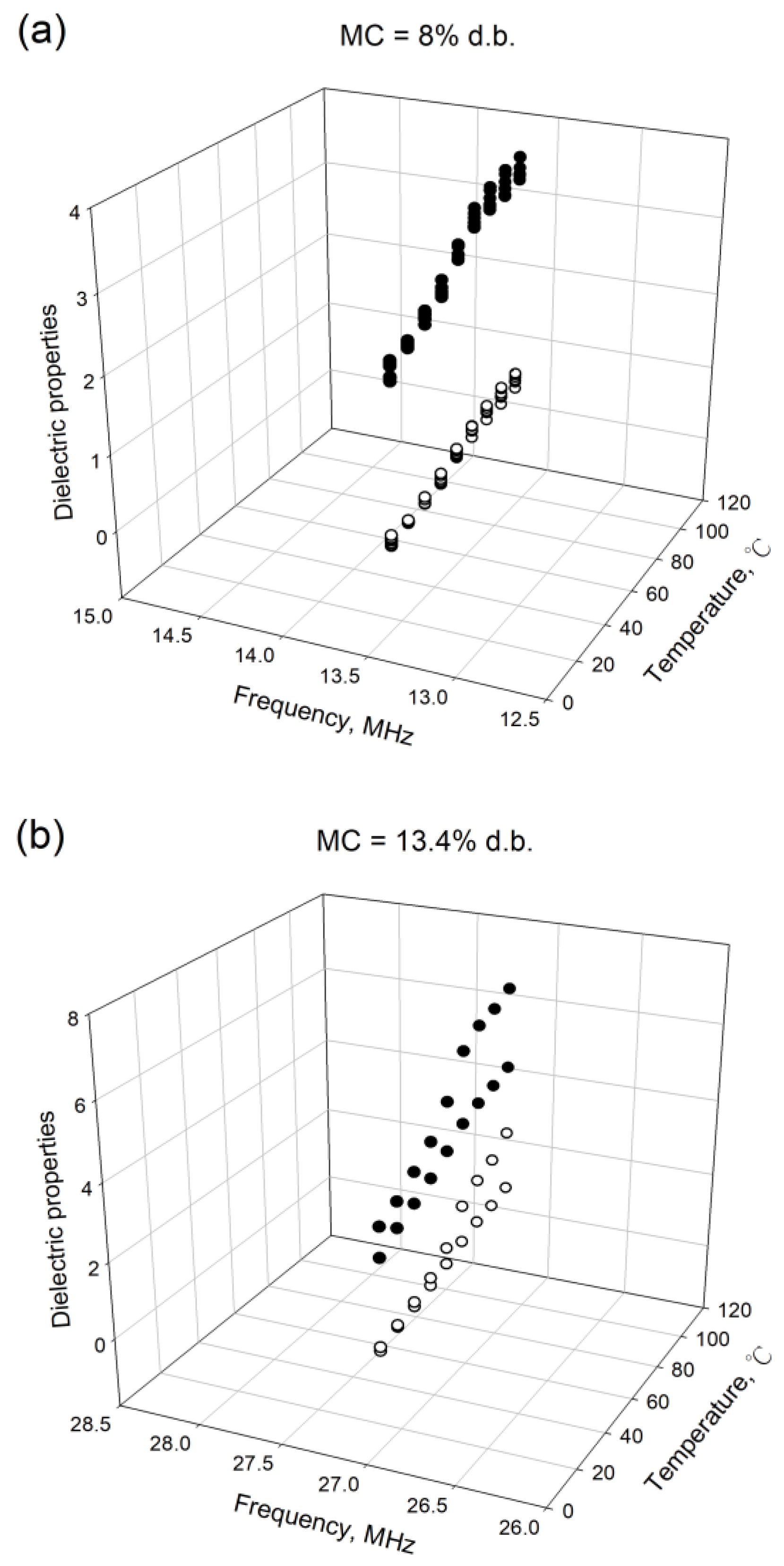
| Egg | White powder | 13.56 | 27.12 | 40.68 | 915 | 2450 | 20 | 40 | 60 | 80 | 100 | 8 | % d.b. | [8] | ||||||||
| 27.12 | 915 | 20 | 40 | 60 | 80 | 100 | 5.5 | 6.6 | 8.0 | 9.8 | 13.4 | % d.b. | ||||||||||
| Whites | Liquid | 27 | 40 | 915 | 1800 | 20 | 40 | 60 | 70 | 80 | 100 | 120 | [9] | |||||||||
| Precooked | ||||||||||||||||||||||
| Egg | Albumen | 10 | 27 | 40 | 100 | 915 | 1800 | 24 | [10] | |||||||||||||
| Yolk | 10 | 27 | 40 | 100 | 915 | 1800 | 24 | Storage time (0,1,2,3,4,5) weeks | ||||||||||||||
| Vegetables | Chickpea flour | 27 | 40 | 100 | 915 | 1800 | 20 | 30 | 40 | 50 | 60 | 70 | 80 | 90 | 7.9 | 11.4 | 15.8 | 20.9 | % w.b. | [11] | ||
| Black-eyed peas | 27 | 40 | 915 | 20 | 30 | 40 | 50 | 60 | 8.8 | 12.7 | 16.8 | 20.9 | % w.b. | [12] | ||||||||
| Fruits | Apple(GD) | 27 | 40 | 915 | 1800 | 20 | 30 | 40 | 50 | 60 | [20] | |||||||||||
| Apple(RD) | ||||||||||||||||||||||
| Cherry | ||||||||||||||||||||||
| Grape-fruit | ||||||||||||||||||||||
| Orange | ||||||||||||||||||||||
| Butter | Unsalted | 915 | 2,450 | 30 | 40 | 50 | 60 | 70 | 80 | [13] | ||||||||||||
| Salted | ||||||||||||||||||||||
| Bread | 13.56 | 27.12 | 40.68 | 915 | 1800 | 25 | 40 | 55 | 70 | 85 | 34.0 | 34.6 | 37.1 | 38.6 | % w.b. | [14] | ||||||
| Cheese | 270 | 500 | 800 | 1200 | 1900 | 3000 | 5 | 45 | 55 | 65 | 75 | 85 | [15] | |||||||||
| Fish | ||||||||||||||||||||||
| Sturgeon caviar | Unsalted | 27 | 915 | 20 | 30 | 40 | 50 | 60 | 70 | 80 | [16] | |||||||||||
| Salted | ||||||||||||||||||||||
| Salmon fillets | Anterior | 27 | 40 | 915 | 1800 | 20 | 40 | 60 | 80 | 100 | 120 | [17] | ||||||||||
| Middle | ||||||||||||||||||||||
| Tail | ||||||||||||||||||||||
| Belly | ||||||||||||||||||||||
| Nut | Almond | 27 | 40 | 915 | 1800 | 20 | 30 | 40 | 50 | 60 | [20] | |||||||||||
| Walnut | 27 | 40 | 915 | 1800 | 20 | 30 | 40 | 50 | 60 | |||||||||||||
| Macadamia nut kernels | 27.12 | 40.68 | 915 | 1800 | 25 | 40 | 60 | 80 | 100 | 3 | 6 | 12 | 18 | 24 | % w.b. | [18] | ||||||
| Pecan | Unsalted | 27 | 40 | 915 | 2450 | 5 | 25 | 45 | 65 | 15 | % w.b. | [19] | ||||||||||
| Light salted | ||||||||||||||||||||||
| Medium salted | ||||||||||||||||||||||
| Heavy salted | ||||||||||||||||||||||
| Insect | Codling moth | 27 | 40 | 915 | 1800 | 20 | 30 | 40 | 50 | 60 | [20] | |||||||||||
| Indian-meal moth | ||||||||||||||||||||||
| Mexican fruit fly | ||||||||||||||||||||||
| Navel arrange worm | ||||||||||||||||||||||
| Equation (3-1): ε′ = 2.928 − (0.0154 × T) − (0.000173 × f) − (0.274 × X) − (0.0000923 × T2) + (0.0151 × X2) + (0.0000353 × T × f) + (0.00558 × T × X) + (0.00000654 × f × X) − (0.00000439 × T × f × X) |
| R2 = 0.980 |
| Normality Test (Kolmogorov–Smirnov): Passed (p = 0.590) |
| Constant Variance Test (Spearman Rank Correlation): Failed (p = 0.041) |
| Equation (3-2): = 1.432 − (0.000287 × T) + (0.0000403 × f) − (0.0340 × X) − (0.0000334 × T2) + (0.00279 × X2) + (0.00000750 × T × f) + (0.00116 × T × X) − (0.00000899 × f × X) − (0.000000906 T × f × X) |
| R2 = 0.980 |
| Normality Test: Passed (p = 0.398) |
| Constant Variance Test: Failed (p = 0.048) |
| Equation (3-3): ln ε′ = 0.488 + (0.00361 × T) + (0.000120 × f) + (0.00237 × X) − (0.0000460 × T2) + (0.00175 × X2) + (0.00000640 × T × f) + (0.000944 × T × X) − (0.0000194 × f × X) − (0.000000743 × T × f × X) |
| R2 = 0.976 |
| Normality Test: Passed (p = 0.160) |
| Constant Variance Test: Passed (p = 0.497) |
| Equation (3-4): 1/ε′ = 0.678 − (0.00330 × T) − (0.0000699 × f) − (0.0219 × X) + (0.0000203 × T2) + (0.000155 × X2) − (0.00000121 × T × f) − (0.000123 × T × X) + (0.0000102 × f × X) + (0.000000119 × T × f × X) |
| R2 = 0.990 |
| Normality Test: Passed (p = 0.151) |
| Constant Variance Test: Passed (p = 0.467) |
| Equation (3-5): ε′ = 2.954 − (0.0456 × T) + (0.0186 × ln f) − (0.282 × X) − (0.0000926 × T2) − (0.00778 × ln f2) + (0.0150× X2) + (0.00928 × T × ln f) + (0.00920 × T × X) + (0.00273 × ln f × X) − (0.00113 × T × ln f) × X) |
| R2 = 0.980 |
| Normality Test: Passed (p = 0.459) |
| Constant Variance Test: Failed (p = 0.003) |
| Equation (3-6): = 1.390 − (0.00697 × T) + (0.0246 × ln f − (0.0291 × X) − (0.0000335 × T2) − (0.00231 × ln f2) + (0.00280 × X2) + (0.00203 × T × ln f + (0.00193 × T × X) − (0.00181 × ln f × X) − (0.000236 × T × ln f × X) |
| R2 = 0.980 |
| Normality Test: Passed (p = 0.355) |
| Constant Variance Test: Failed (p = 0.031) |
| Equation (3-7): ln(ε′) = 0.400 − (0.00242 × T) + (0.0434 × ln f + (0.0140 × X) − (0.0000462 × T2) − (0.00271 × ln f2) + (0.00180 × X2) + (0.00181 × T × ln f + (0.00159 × T × X) − (0.00422 × ln f × X) − (0.000197 × T × ln f × X) |
| R2 = 0.977 |
| Normality Test: Passed (p = 0.370) |
| Constant Variance Test: Passed (p = 0.349) |
| Equation (3-8): 1/ε′ = 0.720 − (0.00196 × T) − (0.0199 × ln f) − (0.0280 × X) + (0.0000204 × T2) + (0.000905 × ln f2) + (0.000118 × X2) − (0.000389 × T × ln f) − (0.000238 × T × X) + (0.00227 × ln f × X) + (0.0000342 × T × ln f × X) |
| R2 = 0.964 |
| Normality Test: Passed (p = 0.020) |
| Constant Variance Test: Passed (p = 0.574) |
| Equation (4-1): ε″ = 1.279 − (0.0230 × T) − (0.000605 × f) − (0.257 × X) − (0.00000381 × T2) + (0.00862 × X2) + (0.0000280 × T × f) + (0.00431 × T × X) + (0.0000899 × f × X) − (0.00000363 × T × f × X) |
| R2 = 0.965 |
| Normality Test: Passed (p = 0.132) |
| Constant Variance Test: Failed |
| Equation (4-2): = 0.124 + (0.00225 × T) + (0.0000236 × f) − (0.0289 × X) − (0.0000489 × T2) + (0.00175 × X2) + (0.00000957 × T × f) + (0.00144 × T × X) + (0.00000852 × f × X) − (0.00000123 × T × f × X) |
| R2 = 0.967 |
| Normality Test: Failed (p = 0.006) |
| Constant Variance Test: Passed (p = 0.064) |
| Equation (4-3): ln(ε″) = -5.742 + (0.0599 × T) + (0.00112 × f) + (0.318 × X) − (0.000316 × T2) − (0.00583 × X2) + (0.00000753 × T × f) + (0.000485 × T × X) − (0.000104 × f × X) − (0.000000957 × T × f × X) |
| R2 = 0.955 |
| Normality Test: Failed (p = < 0.001) |
| Constant Variance Test: Failed (p = < 0.001) |
| Equation (4-4): 1/ε″ = 46.309 − (0.612 × T) − (0.0100 × f) − (4.452 × X) + (0.00259 × T2) + (0.116 × X2) + (0.0000895 × T × f) + (0.0238 × T × X) + (0.00114 × f × X) − (0.0000109 × T × f × X) |
| R2 = 0.712 |
| Normality Test: Failed (p = < 0.001) |
| Constant Variance Test: Failed (p = < 0.001) |
| Equation (4-5): ε″ = 1.667 − (0.0463 × T) − (0.336 × X) − (0.0688 × ln f) − (0.00000442 × T2) − (0.0105 × ln f2) + (0.00875 × X2) + (0.00720 × T × ln f) + (0.00728 × T × X) + (0.0234 × ln f × X) − (0.000923 × T × ln f × X) |
| R2 = 0.963 |
| Normality Test: Passed (p = 0.01) |
| Constant Variance Test: Passed (p = 0.919) |
| Equation (4-6): = 0.115 − (0.00627 × T) − (0.0442 × X) + (0.0458 × ln f) − (0.0000494 × T2) − (0.00647 × ln f2) + (0.00197 × X2) + (0.00259 × T × ln f) + (0.00247 × T × X) + (0.00300 × ln f × X) − (0.000319 × T × ln f × X) |
| R2 = 0.964 |
| Normality Test: Failed (p = 0.004) |
| Constant Variance Test: Passed (p = 0.098) |
| Equation (4-7): ln(ε″) = −6.414 + (0.0504 × T) + (0.369 × X) + (0.342 ×ln f) − (0.000317 × T2) − (0.0153 × ln f2) − (0.00495 × X2) + (0.00264 × T × ln f) + (0.00143 × T × X) − (0.0229 × ln f × X) − (0.000278 × T × ln f × X) |
| R2 = 0.944 |
| Normality Test: Failed (p = < 0.001) |
| Constant Variance Test: Failed (p = < 0.001) |
| Equation (4-8): 1/ε″ = 52.229 − (0.658 × T) − (5.242 × X) − (2.207 × ln f) + (0.00259 × T2) + (0.0108 × ln f2) + (0.114 × X2) + (0.0173 × T × ln f + (0.0312 × T × X) + (0.269 × ln f × X) − (0.00250 × T × ln f × X) |
| R2 = 0.952 |
| Normality Test: Failed (p = < 0.001) |
| Constant Variance Test: Failed (p = < 0.001) |
| Equation (4-9): ε″ = 1.975 − (0.0471 × T) − (0.347 × X) − (0.178 × ln f) + (0.00932 × X2) + (0.00723 × T × ln f) + (0.00729 × T × X) + (0.0236 × ln f × X) − (0.000924 × T × ln f × X) |
| R2 = 0.962 |
| Normality Test: Passed |
| Constant Variance Test: Passed (p = 0.823) |
| Equation (5-1): ln(ε′) = 2.521 − (0.0201 × T) − (0.195 × X) + (0.0184 × ln f) + (0.000242 × T2) − (0.000327 × ln f2) + (0.00926 × X2) + (0.000677 × T × ln f) + (0.000693 × T × X) − (0.00662 × ln f × X) − (0.0000247 × T × ln f × X) − (0.00000124 × (T × X) 2) |
| R2 = 0.940 |
| Normality Test: Passed (p = 0.310) |
| Constant Variance Test: Passed (p = 0.975) |
| Equation (5-2): 1/ε′ = 0.150 + (0.000411 × T) + (0.0268 × X) − (0.00544 × ln f) − (0.0000337 × T2) + (0.00136 × ln f2) − (0.00142 × X2) + (0.000264 × T × ln f) + (0.0000185 × T × X) + (0.000664 × ln f × X) − (0.0000119 × T × ln f × X) − (0.000000108 × (T × X) 2) |
| R2 = 0.928 |
| Normality Test: Passed (p = 0.082) |
| Constant Variance Test: Passed (p = 0.897) |
| Equation (5-3): ln(ε″) = 4.531 − (0.0719 × T) − (0.375 × X) − (1.349 × ln f) + (0.000639 × T2) + (0.0909 × ln f2) + (0.0131 × X2) + (0.00674 × T × ln f) + (0.00315 × T × X) + (0.0161 × ln f × X) − (0.0000621 × T × ln f × X) − (0.00000770 × T × ln f2) − (0.000000970 × (T × X) 2) |
| R2 = 0.952 |
| Normality Test: Passed (p = 0.158) |
| Constant Variance Test: Passed (p = 0.197) |
| Equation (6-1): ln(ε′) = 1.467 − (0.000659 × T) + (0.102 × X) − (0.119 × ln f) + (0.0000327 × T2) + (0.0170 × ln f2) + (0.00000963 × X2) − (0.000227 × T × ln f) + (0.000304 × T × X) − (0.00904 × ln f × X) - (0.00000325 × T × ln f × X) − (0.000000205 × T × ln f2) − (0.0000000679 × (T × X)2) |
| R2 = 0.952 |
| Normality Test: Passed (p = 0.171) |
| Constant Variance Test: Failed (p = < 0.001) |
| Equation (6-2): ln(ε″) = -1.719 + (0.00660 × T) + (0.469 × X) − (0.351 × ln f) + (0.0000602 × T2) + (0.0627 × ln f2) − (0.00381 × X2) − (0.00102 × T × ln f) + (0.000778 × T × X) − (0.0397 × ln f × X) - (0.000118 × T × ln f × X) + (0.000000144 × (T × X)2) |
| R2 = 0.959 |
| Normality Test: Passed (p = 0.165) |
| Constant Variance Test: Passed (p = 0.711) |
| 1. Gold Apple |
| Equation (7-1): ln(ε′) = 3.691 − (0.000619 × T) + (0.269 × ln f) − (0.0000114 × T2) − (0.0256 × ln f2) − (0.000206 × T × ln f) |
| R2 = 0.900 |
| Normality Test: Passed (p = 0.637) |
| Constant Variance Test: Passed (p = 0.235) |
| Equation (7-2): 1/ε′ = 0.0228 + (0.00000228 × T) − (0.00404 × ln f) + (0.000000220 × T2) + (0.000382 × ln f2) + (0.00000354 × T × ln f) |
| R2 = 0.901 |
| Normality Test: Passed (p = 0.331) |
| Constant Variance Test: Passed (p = 0.402) |
| Equation (7-3): ln(ε″) = 10.015 + (0.0348 × T) − (2.176 × ln f) + (0.0000411 × T2) + (0.154 × ln f2) − (0.00604 × T × ln f) |
| R2 = 0.997 |
| Normality Test: Passed (p = 0.131) |
| Constant Variance Test: Passed (p = 0.011) |
| 2. Red Apple |
| Equation (7-4): ln(ε′) = 3.788 − (0.00239 × T) + (0.251 × ln f) + (0.000000945 × T2) − (0.0237 × ln f2) − (0.000144 × T × ln f) |
| R2 = 0.926 |
| Normality Test: Passed (p = 0.662) |
| Constant Variance Test: Passed (p = 0.021) |
| Equation (7-5): = 25.153 + (0.175 × T) − (7.248 × ln f) + (0.0000614 × T2) + (0.588 × ln f2) − (0.0265 × T × ln f) |
| R2 = 0.996 |
| Normality Test: Passed (p = 0.022) |
| Constant Variance Test: Passed (p = 0.131) |
| 3. Cherry |
| Equation (7-6): ε′ = 142.581 + (0.120 × T) − (21.083 × ln f) − (0.00145 × T2) + (1.624 × ln f2) − (0.0322 × T × ln f) |
| R2 = 0.936 |
| Normality Test: Passed (p = 0.153) |
| Constant Variance Test: Passed (p = 0.343) |
| Equation (7-7): = 12.262 + (0.00874 × T) − (1.118 × ln f) − (0.0000921 × T2) + (0.0858 × ln f2) − (0.00211 × T × ln f) |
| R2 = 0.941 |
| Normality Test: Passed (p = 0.284) |
| Constant Variance Test: Passed (p = 0.738) |
| Equation (7-8): ln(ε′) = 5.083 + (0.00246 × T) − (0.236 × ln f) − (0.0000234 × T2) + (0.0181 × ln f2) − (0.000546 × T × ln f) |
| R2 = 0.946 |
| Normality Test: Passed (p = 0.433) |
| Constant Variance Test: Passed (p = 0.933) |
| Equation (7-9): 1/ε′ = 0.00479 − (0.0000451 × T) + (0.00261 × ln f) + (0.000000376 × T2) − |
| (0.000199 × ln f2) + (0.00000895 × T × ln f) |
| R2 = 0.954 |
| Normality Test: Passed (p = 0.538) |
| Constant Variance Test: Passed (p = 0.518) |
| Equation (7-10): 1/ε″ = 0.0900 + (0.00195 × T) − (0.0577 × ln f) − (0.0000305 × T2) + (0.00618 × ln f2) + (0.000135 × T × ln f) |
| R2 = 0.881 |
| Normality Test: Passed (p = 0.019) |
| Constant Variance Test: Passed (p = 0.251) |
| 4. Grapefruit |
| Equation (7-11): = 13.036 + (0.0174 × T) − (1.566 × ln f) + (0.0000179 × T2) + (0.136 × ln f2) −(0.00449 × T × ln f)) |
| R2 = 0.823 |
| Normality Test: Passed (p = 0.024) |
| Constant Variance Test: Failed (p = < 0.001) |
| Equation (7-12): ln(ε″) = 9.996 + (0.0334 × T) − (1.926 × ln f) + (0.122 × ln f2) − (0.00455 × T × ln f) |
| R2 = 0.998 |
| Normality Test: Passed (p = 0.495) |
| Constant Variance Test: Passed (p = 0.165) |
| Equation (7-13): 1/ε″ = -0.0353 + (0.000122 × T) + (0.00677 × ln f) − (0.00000400 × T2) + (0.00124 × ln f2) + (0.0000249 × T × ln f) |
| R2 = 0.986 |
| Normality Test: Passed (p = 0.324) |
| Constant Variance Test: Passed (p = 0.030) |
| 5. Orange |
| Equation (7-14): ε′ = 123.333 − (0.159 × T) − (14.544 × ln f) − (0.000964 × T2) + (1.114 × ln f2) − (0.00126 × T × ln f) |
| R2 = 0.968 |
| Normality Test: Passed (p = 0.592) |
| Constant Variance Test: Passed (p = 0.229) |
| Equation (7-15): = 11.381 − (0.00702 × T) − (0.828 × ln f) − (0.0000692 × T2) + (0.0640 × ln f2) − (0.000325 × T × ln f) |
| R2 = 0.969 |
| Normality Test: Passed (p = 0.311) |
| Constant Variance Test: Passed (p = 0.157) |
| Equation (7-16): ln(ε′) = 4.930 − (0.00110 × T) − (0.188 × ln f) − (0.0000193 × T2) + (0.0147 × lnf2) − (0.000135 × T × ln f) |
| R2 = 0.969 |
| Normality Test: Passed (p = 0.257) |
| Constant Variance Test: Passed (p = 0.089) |
| Equation (7-17): 1/ε′ = 0.00560 + (0.0000000811 × T) + (0.00244 × ln f) + (0.000000351 × T2) − (0.000194 × ln f2) + (0.00000351 × T × ln f) |
| R2 = 0.970 |
| Normality Test: Passed (p = 0.049)Constant Variance Test: Passed (p = 0.033) |
| Equation (7-18): ln(ε″) = 8.981 + (0.0369 × T) − (1.486 × ln f) − (0.0000568 × T2) + (0.0850 × lnf2) − (0.00474 × T × ln f) |
| R2 = 0.998 |
| Normality Test: Passed (p = 0.075) |
| Constant Variance Test: Passed (p = 0.062) |
| 6. Almond |
| Equation (7-19): = 5.816 − (0.00407 × T) − (1.357 × ln f) + (0.0000683 × T2) + (0.112 × ln f2) |
| R2 = 0.381 |
| Normality Test: Passed (p = 0.179) |
| Constant Variance Test: Passed (p = 0.133) |
| Equation (7-20): = −6.515 − (0.0200 × T) + (3.221 × ln f) + (0.000132 × T2) − (0.278 ×ln f2) +(0.00144 × T× ln f) |
| R2 = 0.879 |
| Normality Test: Passed (p = 0.120) |
| Constant Variance Test: Passed (p = 0.605) |
| Equation (7-21): ln(ε″) = −8.572 − (0.0505 × T) + (3.826 × ln f) + (0.000401 × T2) − (0.328 × ln f2) + (0.00268 × T × ln f) |
| R2 = 0.878 |
| Normality Test: Passed (p = 0.016) |
| Constant Variance Test: Passed (p = 0.030) |
| 7. Walnut |
| Equation (7-22): ε′ = 11.067 − (0.0193 × T) − (2.308 × ln f) + (0.132 × ln f2) + (0.00855 × T × ln f) |
| R2 = 0.957 |
| Normality Test: Passed (p = 0.046) |
| Constant Variance Test: Passed (p = 0.313) |
| Equation (7-23): = 3.861 − (0.00278 × T) − (0.639 × ln f) − (0.0000549 × T2) + (0.0361 × ln f2) + (0.00274 × T × ln f) |
| R2 = 0.941 |
| Normality Test: Passed (p = 0.028) |
| Constant Variance Test: Passed (p = 0.386) |
| Equation (7-24): = −3.502 − (0.00606 × T) + (1.810 ×ln f) + (0.0000854 × T2) − (0.149 × ln f2) − (0.00136 × T × ln f) |
| R2 = 0.936 |
| Normality Test: Passed (p = 0.058) |
| Constant Variance Test: Passed (p = 0.084) |
| Equation (7-25): ln(ε″) = −7.867 − (0.0248 × T) + (3.187 × ln f) + (0.000201 × T2) − (0.264 × ln f2) − (0.000704 × T × ln f) |
| R2 = 0.944 |
| Normality Test: Passed (p = 0.190) Constant Variance Test: Passed (p = 0.559) |
| 8. Codling Moth |
| Equation (7-26): ε′ = 127.988 + (0.0726 × T) − (22.820 × ln f) + (0.00609 × T2) + (1.757 × ln f2) − (0.0863 × T × ln f) |
| R2 = 0.976 |
| Normality Test: Passed (p = 0.112) |
| Constant Variance Test: Passed (p = 0.159) |
| Equation (7-27): ln(ε″) = 10.615 + (0.0186 × T) − (2.044 × ln f) + (0.000174 × T2) + (0.127 × ln f2) − (0.00339 × T × ln f) |
| R2 = 0.997 |
| Normality Test: Passed (p = 0.390) |
| Constant Variance Test: Passed (p = 0.748) |
| 9. Indian-Meal Moth |
| Equation (7-28): = 15.431 + (0.0545 × T) − (2.853 × ln f) + (0.000248 × T2) + (0.226 × ln f2) − (0.0110 × T × ln f) |
| R2 = 0.993 |
| Normality Test: Passed (p = 0.137) |
| Constant Variance Test: Passed (p = 0.015) |
| Equation (7-29): ln(ε′) = 5.885 + (0.0117 × T) − (0.640 × ln f)) + (0.0000574 × T2) + (0.0478 × ln f2) − (0.00249 × T × ln f) |
| R2 = 0.996 |
| Normality Test: Passed (p = 0.355) |
| Constant Variance Test: Passed (p = 0.939) |
| Equation (7-30): ln(ε″) = 9.086 + (0.00878 × T) − (1.360 × ln f) + (0.000180 × T2) + (0.0626 × ln f2) − (0.00229 × T × ln f) |
| R2 = 0.996 |
| Normality Test: Passed (p = 0.296) |
| Constant Variance Test: Passed (p = 0.779) |
| 10. Mexican Fruit Fly |
| Equation (7-31): ε′−1.5 = -0.00167 − (0.0000389 × T) + (0.00125 × ln f) − (0.0000862 × ln f2) + (0.00000678 × T × ln f) |
| R2 = 0.965 |
| Normality Test: Passed (p = 0.661) |
| Constant Variance Test: Passed (p = 0.014) |
| Equation (7-32): ε″ = 1222.142 + (9.378 × T) − (417.002 ×ln f) + (0.0120 × T2) + (34.831 × ln f2) − (1.417 × T × ln f) |
| R2 = 0.985 |
| Normality Test: Passed (p = 0.428) |
| Constant Variance Test: Passed (p = 0.159) |
| 11. Navel Orange Worm |
| Equation (7-33): 1/ε′ = -0.00500 − (0.0000968 × T) + (0.00703 × ln f) − (0.000000520 × T2) − (0.000456 × ln f2) + (0.0000238 × T × ln f) |
| R2 = 0.997 |
| Normality Test: Passed (p = 0.229) |
| Constant Variance Test: Passed (p = 0.126) |
| Equation (7-34): ln(ε″) = 9.662 + (0.0225 × T) − (1.520 ×ln f)) + (0.0725 × ln f2) − (0.00213 × T × ln f) |
| R2 = 0.999 |
| Normality Test: Passed (p = 0.447) |
| Constant Variance Test: Passed (p = 0.741) |
| 1. Egg Yolk | ||||||
| Equation (8-1): ln(ε′) = 5.722 − (0.661 × ln f) + (0.0498 × ln f2) | ||||||
| R2 = 0.967 | ||||||
| Normality Test: Passed (p = 0.451) | ||||||
| Constant Variance Test: Passed (p = 0.270) | ||||||
| Equation (8-2): ln(ε′) = 5.717 − (0.00498 × St) − (0.664 × ln f)) + (0.00198 × St2) + (0.0498 × ln f2) +(0.000975 × St × ln f) | ||||||
| R2 = 0.970 | ||||||
| Coefficient | Std. Error | t | p | |||
| Constant | 5.717 | 0.106 | 53.775 | <0.001 | ||
| St | −0.00498 | 0.0269 | −0.185 | 0.854 | ||
| ln f | −0.664 | 0.0441 | −15.051 | <0.001 | ||
| St2 | 0.00198 | 0.00422 | 0.468 | 0.643 | ||
| ln f2 | 0.0498 | 0.00427 | 11.644 | <0.001 | ||
| St× ln f | 0.000975 | 0.00329 | 0.297 | 0.769 | ||
| Equation (8-3): ln(ε″) = 9.088 − (1.315 × ln f)) + (0.0520 × ln f2) | ||||||
| R2 = 0.998 | ||||||
| Equation (8-4): ln(ε″) = 9.087 − (0.00768 × St) − (1.318 × ln f) + (0.00210 × St2) + (0.0520 × ln f2) + (0.00113 × St × ln f) | ||||||
| R2 = 0.998 | ||||||
| Coefficient | Std. Error | t | p | |||
| Constant | 9.087 | 0.109 | 83.221 | <0.001 | ||
| St | −0.00768 | 0.0276 | −0.278 | 0.783 | ||
| ln f | −1.318 | 0.0453 | −29.089 | <0.001 | ||
| St2 | 0.00210 | 0.00433 | 0.484 | 0.632 | ||
| ln f2 | 0.0520 | 0.00439 | 11.833 | <0.001 | ||
| St× ln f | 0.00113 | 0.00338 | 0.336 | 0.739 | ||
| 2. Albumen | ||||||
| Equation (8-5): ln(ε′) = 6.269 − (0.721 × ln f) + (0.0604 × ln f2) | ||||||
| R2 = 0.898 | ||||||
| Equation (8-6): ln(ε′) = 6.275 − (0.0216 × St) − (0.718 × ln f) + (0.00523 × St2) + (0.0604 × ln f2) – (0.00126 × St × ln f) | ||||||
| R2 = 0.901 | ||||||
| Equation (8-7): ln(ε″) = 10.077 − (1.300 × ln f) + (0.0425 × ln f2) | ||||||
| R2 = 0.999 | ||||||
| Equation (8-8): ln(ε″) = 10.052 − (0.0107 × St) − (1.297 × ln f) + (0.000141 × St2) + (0.0425 × ln f2) – (0.00108 × St × ln f) | ||||||
| R2 = 0.999 | ||||||
| Coefficient | Std. Error | t | p | |||
| Constant | 10.052 | 0.106 | 94.628 | <0.001 | ||
| St | 0.0107 | 0.0268 | 0.398 | 0.693 | ||
| ln f | −1.297 | 0.0441 | −29.432 | <0.001 | ||
| St2 | −0.000141 | 0.00421 | −0.0335 | 0.973 | ||
| ln f2 | 0.0425 | 0.00427 | 9.956 | <0.001 | ||
| St× ln f | −0.00108 | 0.00329 | −0.328 | 0.745 | ||
| 1. Butter (Salted and Unsalted) | ||||||
| Equation (9-1): ln(ε′) = 3.777 + (1.370 × z) + (0.00355 × T) + (0.00433 × T × z) − (0.000160 × T2) + (0.000151 × T2 × z) − (0.0680 × ln f) − (0.349 × ln f × z) | ||||||
| R2 = 0.965 | ||||||
| Coefficient | Std. Error | t | p | |||
| Constant | 3.777 | 0.206 | 18.342 | <0.001 | ||
| z | 1.370 | 0.291 | 4.706 | <0.001 | ||
| T | 0.00355 | 0.00488 | 0.728 | 0.470 | ||
| T × z | 0.00433 | 0.00691 | 0.627 | 0.533 | ||
| T2 | −0.000160 | 0.0000440 | −3.647 | <0.001 | ||
| T2 × z | 0.000151 | 0.0000622 | 2.424 | 0.018 | ||
| ln f | −0.0680 | 0.0223 | −3.049 | 0.003 | ||
| ln f × z | −0.349 | 0.0315 | −11.065 | <0.001 | ||
| Equation (9-2): ln ε″ = 3.978 + (19.066 × z) − (0.0126 × T) + (0.0902 × T × z) − (0.00000579 × T2) − (0.000241 × T2 × z) − (0.192 × ln f) − (2.600 × ln f2 × z) | ||||||
| R2 = 0.989 | ||||||
| Coefficient | Std. Error | t | p | |||
| Constant | 3.978 | 0.851 | 4.674 | <0.001 | ||
| z | 19.066 | 1.204 | 15.839 | <0.001 | ||
| T | −0.0126 | 0.0202 | −0.623 | 0.536 | ||
| T × z | 0.0902 | 0.0285 | 3.158 | 0.002 | ||
| T2 | −0.00000579 | 0.000182 | −0.0318 | 0.975 | ||
| T2 × z | −0.000241 | 0.000257 | −0.935 | 0.353 | ||
| ln f | −0.192 | 0.0921 | −2.081 | 0.041 | ||
| ln f × z | −2.600 | 0.130 | −19.950 | <0.001 | ||
| 2. Salmon Fish (Salted and Unsalted) | ||||||
| Equation (9-3): = 12.759 + (6.579 × z) − (0.117 × T) + (0.0296 × T × z) + (0.00105 × T2) − (0.790 × ln f) − (1.128 × ln f × z) | ||||||
| R2 = 0.912 | ||||||
| Coefficient | Std. Error | t | p | |||
| Constant | 12.759 | 0.837 | 15.249 | <0.001 | ||
| z | 6.579 | 0.800 | 8.221 | <0.001 | ||
| T | −0.117 | 0.0302 | −3.887 | <0.001 | ||
| T × z | 0.0296 | 0.0102 | 2.911 | 0.005 | ||
| T2 | 0.00105 | 0.000293 | 3.576 | <0.001 | ||
| ln f | −0.790 | 0.0816 | −9.680 | <0.001 | ||
| ln f × z | −1.128 | 0.115 | −9.769 | <0.001 | ||
| Equation (9-4): ln ε″ = 9.649 + (1.244 × z) − (0.0301 × T) + (0.00760 × T × z) + (0.000343 × T2) − (0.935 × ln f) − (0.0831 × ln f × z) | ||||||
| R2 = 0.973 | ||||||
| Coefficient | Std. Error | t | p | |||
| Constant | 9.649 | 0.288 | 33.473 | <0.001 | ||
| z | 1.244 | 0.276 | 4.513 | <0.001 | ||
| T | −0.0301 | 0.0104 | −2.896 | 0.005 | ||
| T × z | 0.00760 | 0.00350 | 2.170 | 0.033 | ||
| T2 | 0.000343 | 0.000101 | 3.396 | 0.001 | ||
| ln f | −0.935 | 0.0281 | −33.245 | <0.001 | ||
| ln f × z | −0.0831 | 0.0398 | −2.090 | 0.040 | ||
| Moisture Content of Cheese: High, Medium and Low | ||||||
|---|---|---|---|---|---|---|
| Equation (10-1): = 8.985 + (0.715 × z1) + (0.168 × z2) − (0.0322 × T) + (0.000270 × T2) − (0.494 × ln f) + (0.0231 × T × z1) − (0.000224 × T2 × z3) + (0.0183 × T × z2) − (0.000142 × T2 × z2) | ||||||
| R2 = 0.932 | ||||||
| Coefficient | Std. Error | t | p | |||
| Constant | 8.985 | 0.173 | 52.025 | <0.001 | ||
| z1 | 0.715 | 0.122 | 5.875 | <0.001 | ||
| z2 | 0.168 | 0.123 | 1.362 | 0.176 | ||
| T | −0.0322 | 0.00461 | −6.978 | <0.001 | ||
| T2 | 0.000270 | 0.0000495 | 5.446 | <0.001 | ||
| ln f | −0.494 | 0.0218 | −22.714 | <0.001 | ||
| T × z1 | 0.0231 | 0.00625 | 3.693 | <0.001 | ||
| T2 × z1 | −0.000224 | 0.0000674 | −3.326 | 0.001 | ||
| T × z2 | 0.0183 | 0.00652 | 2.807 | 0.006 | ||
| T2 × z2 | −0.000142 | 0.0000701 | −2.023 | 0.046 | ||
| Equation (10-2): = 22.116 + (2.584 × z1) − (10.126 × z2) + (0.0445 × T) − (0.975 × T2) − (2.178 × ln f) − (0.0293 × T × z1) + (0.864 × T2 × z1) − (0.437 × ln f × z1) − (0.0335 × T × z2) + (0.928 × T2 × z2) + (1.143 × ln f × z2) | ||||||
| R2 = 0.936 | ||||||
| Coefficient | Std. Error | t | p | |||
| Constant | 22.116 | 0.953 | 23.203 | <0.001 | ||
| z1 | 2.584 | 1.351 | 1.913 | 0.059 | ||
| z2 | −10.126 | 1.366 | −7.412 | <0.001 | ||
| T | 0.0445 | 0.00910 | 4.886 | <0.001 | ||
| T2 | −0.975 | 0.252 | −3.863 | <0.001 | ||
| ln f | −2.178 | 0.113 | −19.273 | <0.001 | ||
| T × z1 | −0.0293 | 0.0128 | −2.282 | 0.025 | ||
| T2 × z1 | 0.864 | 0.357 | 2.420 | 0.018 | ||
| ln f × z1 | −0.437 | 0.160 | −2.733 | 0.008 | ||
| T × z2 | −0.0335 | 0.0129 | −2.591 | 0.011 | ||
| T2 × z2 | 0.928 | 0.360 | 2.579 | 0.012 | ||
| ln f × z2 | 1.143 | 0.163 | 7.009 | <0.001 | ||
| Position: Anterior, Middle, Tail, Belly | ||||||
|---|---|---|---|---|---|---|
| Equation (11-1): ln(ε′) = 5.719 − (0.0802 × z1) + (0.0703 × z2) + (0.0585 × z3) + (0.00917 × T) − (0.487 × ln f) + (0.0352 × ln f2) − (0.00160 × T × ln f) + (0.000522 × T × z1) + (0.000684 × T × z3) + (0.0140 × ln f × z1) − (0.0160 × ln f × z3) | ||||||
| R2 = 0.973 | ||||||
| Coefficient | Std. Error | t | p | |||
| Constant | 5.719 | 0.0693 | 82.472 | <0.001 | ||
| z1 | −0.0802 | 0.0352 | −2.277 | 0.023 | ||
| z2 | 0.0703 | 0.0101 | 6.936 | <0.001 | ||
| z3 | 0.0585 | 0.0352 | 1.660 | 0.098 | ||
| T | 0.00917 | 0.000372 | 24.652 | <0.001 | ||
| ln f | −0.487 | 0.0265 | −18.371 | <0.001 | ||
| ln f2 | 0.0352 | 0.00245 | 14.334 | <0.001 | ||
| T × ln f | −0.00160 | 0.0000623 | −25.612 | <0.001 | ||
| T × z1 | 0.000522 | 0.000257 | 2.029 | 0.043 | ||
| T × z3 | 0.000684 | 0.000257 | 2.659 | 0.008 | ||
| ln f × z1 | 0.0140 | 0.00522 | 2.685 | 0.008 | ||
| ln f × z3 | −0.0160 | 0.00522 | −3.066 | 0.002 | ||
| Equation (11-2): ln(ε″) = 6.368 − (0.341 × z1) − (0.0207 × z2) − (0.389 × z3) − (0.00129 × T) − (0.844 × ln f) + (0.179 × ln f2) − (0.000154 × T × ln f) + (0.105 × ln f × z1) + (0.0223 × ln f × z2) + (0.0743 × ln f × z3) | ||||||
| R2 = 0.766 | ||||||
| Coefficient | Std. Error | t | p | |||
| Constant | 6.368 | 1.870 | 3.405 | <0.001 | ||
| z1 | −0.341 | 0.749 | −0.455 | 0.650 | ||
| z2 | −0.0207 | 0.749 | −0.0276 | 0.978 | ||
| z3 | −0.389 | 0.749 | −0.520 | 0.603 | ||
| T | −0.00129 | 0.000399 | −3.220 | 0.001 | ||
| ln f | −0.844 | 0.949 | −0.890 | 0.374 | ||
| ln f2 | 0.179 | 0.121 | 1.485 | 0.138 | ||
| T × ln f | −0.000154 | 0.0000965 | −1.593 | 0.112 | ||
| ln f × z1 | 0.105 | 0.180 | 0.580 | 0.562 | ||
| ln f × z2 | 0.0223 | 0.181 | 0.123 | 0.902 | ||
| ln f × z3 | 0.0743 | 0.1801 | 0.411 | 0.682 | ||
| Treatments: No Salted, Light Salted, Medium Salted and Heavy Salted | ||||||
|---|---|---|---|---|---|---|
| Equation (12-1): ln(ε′) = 2.150 − (0.533 × z1) − (14.653 × z2) − (8.721 × z3) + (0.000199 × T) + (0.138 × ln f) − (0.0287 × ln f2) + (0.000000720 × T2) − (0.000602 × T × ln f) + (0.0257 × T × z1) − (0.000158 × T × z3) + (6.999 × ln f× z2) + (4.786 × ln f × z3) − (0.661 × ln f2 × z2) − (0.468 × ln f2 × z3) | ||||||
| R2 = 0.625 | ||||||
| Coefficient | Std. Error | t | p | |||
| Constant | 2.150 | 2.034 | 1.057 | 0.291 | ||
| z1 | −0.533 | 0.321 | −1.661 | 0.098 | ||
| z2 | −14.653 | 2.708 | −5.411 | <0.001 | ||
| z3 | −8.721 | 2.495 | −3.495 | <0.001 | ||
| T | 0.000199 | 0.000857 | 0.232 | 0.817 | ||
| ln f | 0.138 | 0.840 | 0.164 | 0.870 | ||
| ln f2 | −0.0287 | 0.0765 | −0.375 | 0.708 | ||
| T2 | 0.00000072 | 0.000000235 | 3.060 | 0.002 | ||
| T × ln f | −0.000602 | 0.000181 | −3.327 | <0.001 | ||
| T × z1 | 0.0257 | 0.00681 | 3.781 | <0.001 | ||
| T × z3 | −0.000158 | 0.000220 | −0.718 | 0.473 | ||
| ln f × z2 | 6.999 | 1.094 | 6.397 | <0.001 | ||
| ln f × z3 | 4.786 | 1.022 | 4.684 | <0.001 | ||
| ln f2 × z2 | −0.661 | 0.0991 | −6.667 | <0.001 | ||
| ln f2 × z3 | −0.468 | 0.0932 | −5.022 | <0.001 | ||
| Equation (12-2): ln(ε″) = -7.341 + (6.370 × z1) − (4.537 × z2) + (2.928 × z3) − (0.00236 × T) + (4.163 × ln f) − (0.448 × ln f2) + (0.000000707 × T2) + (0.0000175 × T × ln f) + (0.0321 × T × z1) − (3.082 × ln f × z1) + (2.987 × ln f × z2) + (0.302 ×ln f2 × z1) − (0.281 × ln f2 × z2) | ||||||
| R2 = 0.694 | ||||||
| Coefficient | Std. Error | t | p | |||
| Constant | −7.341 | 1.276 | −5.755 | <0.001 | ||
| z1 | 6.370 | 3.322 | 1.918 | 0.056 | ||
| z2 | −4.537 | 2.110 | −2.150 | 0.032 | ||
| z3 | 2.928 | 0.204 | 14.335 | <0.001 | ||
| T | −0.00236 | 0.000453 | −5.215 | <0.001 | ||
| ln f | 4.163 | 0.532 | 7.827 | <0.001 | ||
| ln f2 | −0.448 | 0.0503 | −8.903 | <0.001 | ||
| T2 | 0.000000707 | 0.000000251 | 2.81 | 0.005 | ||
| T × ln f | 0.0000175 | 0.00000289 | 6.059 | <0.001 | ||
| T × z1 | 0.0321 | 0.00767 | 4.182 | <0.001 | ||
| ln f × z1 | −3.082 | 1.371 | −2.249 | 0.025 | ||
| ln f × z2 | 2.987 | 0.836 | 3.575 | <0.001 | ||
| ln f2 × z1 | 0.302 | 0.125 | 2.413 | 0.016 | ||
| ln f2 × z2 | −0.281 | 0.0756 | −3.723 | <0.001 | ||
Publisher’s Note: MDPI stays neutral with regard to jurisdictional claims in published maps and institutional affiliations. |
© 2020 by the authors. Licensee MDPI, Basel, Switzerland. This article is an open access article distributed under the terms and conditions of the Creative Commons Attribution (CC BY) license (http://creativecommons.org/licenses/by/4.0/).
Share and Cite
Weng, Y.-K.; Chen, J.; Cheng, C.-W.; Chen, C. Use of Modern Regression Analysis in the Dielectric Properties of Foods. Foods 2020, 9, 1472. https://doi.org/10.3390/foods9101472
Weng Y-K, Chen J, Cheng C-W, Chen C. Use of Modern Regression Analysis in the Dielectric Properties of Foods. Foods. 2020; 9(10):1472. https://doi.org/10.3390/foods9101472
Chicago/Turabian StyleWeng, Yu-Kai, Jiunyuan Chen, Ching-Wei Cheng, and Chiachung Chen. 2020. "Use of Modern Regression Analysis in the Dielectric Properties of Foods" Foods 9, no. 10: 1472. https://doi.org/10.3390/foods9101472
APA StyleWeng, Y.-K., Chen, J., Cheng, C.-W., & Chen, C. (2020). Use of Modern Regression Analysis in the Dielectric Properties of Foods. Foods, 9(10), 1472. https://doi.org/10.3390/foods9101472