You are currently viewing a new version of our website. To view the old version click .
Foods
  • Article
  • Open Access

20 April 2023

Rapid Test for Adulteration of Fritillaria Thunbergii in Fritillaria Cirrhosa by Laser-Induced Breakdown Spectroscopy

,
,
,
,
,
,
,
,
and
1
School of Optics and Photonics, Beijing Institute of Technology, Beijing 100081, China
2
Key Laboratory of Photonic Information Technology, Ministry of Industry and Information Technology, Beijing Institute of Technology, Beijing 100081, China
3
Department of Engineering Science, Institute of Biomedical Engineering, University of Oxford, Oxford OX3 7LD, UK
4
Yangtze Delta Region Academy of Beijing Institute of Technology, Jiaxing 314033, China
This article belongs to the Section Food Analytical Methods

Abstract

Fritillaria has a long history in China, and it can be consumed as medicine and food. Owing to the high cost of Fritillaria cirrhosa, traders sometimes mix it with the cheaper Fritillaria thunbergii powder to make profit. Herein, we proposed a laser-induced breakdown spectroscopy (LIBS) technique to test the adulteration present in the sample of Fritillaria cirrhosa powder. Experimental samples with different adulteration levels were prepared, and their LIBS spectra were obtained. Partial least squares regression (PLSR) was adopted as the quantitative analysis model to compare the effects of four data standardization methods, namely, mean centring, normalization by total area, standard normal variable, and normalization by the maximum, on the performance of the PLSR model. Principal component analysis and least absolute shrinkage and selection operator (LASSO) were utilized for feature extraction and feature selection, and the performance of the PLSR model was determined based on its quantitative analysis. Subsequently, the optimal number of features was determined. The residuals were corrected using support vector regression (SVR). The mean absolute error and root mean square error of prediction obtained from the quantitative analysis results of the combined LASSO-PLSR-SVR model for the test set data were 5.0396% and 7.2491%, respectively, and the coefficient of determination R2 was 0.9983. The results showed that the LIBS technique can be adopted to test adulteration in the sample of Fritillaria cirrhosa powder and has potential applications in drug quality control.

1. Introduction

Fritillaria has high medicinal value because of its ability to moisten the lungs, relieve cough, reduce phlegm, and it can also be consumed as a food [1,2]. Owing to the difference in efficacy and supply and demand, the price of Fritillaria cirrhosa is several times higher than other Fritillaria varieties [3]. In the market, unscrupulous merchants sometimes mix cheaper Fritillaria powders with Fritillaria cirrhosa powder and attempt to sell them off as pure Fritillaria cirrhosa. Therefore, it is necessary to develop a rapid and convenient method to test the level of adulteration of other Fritillaria powders in Fritillaria cirrhosa powder samples [4]. In this paper, the adulteration of Fritillaria thunbergii powder in Fritillaria cirrhosa powder was tested.
Currently, these techniques, such as atomic absorption spectrometry (AAS), inductively-coupled plasma-mass spectrometry (ICP-MS), and inductively-coupled plasma optical emission spectrometry (ICP-OES), can be utilized to quantitatively analyse pharmaceutical products; however, these conventional analysis techniques require complex and time-consuming pre-treatments, such as high temperature and high acid digestion [5]. Fluorescence, Raman, and near-infrared spectroscopies are the most prevalent spectroscopic detection techniques. When adopting these techniques, sample processing is complex and time consuming, and weak spectral signals are susceptible to background light, which prevents in situ, real-time, and rapid online detection [6].
Laser-induced breakdown spectroscopy (LIBS) is an atomic emission spectroscopy technique with the advantages of in situ, real-time, rapid, and simultaneous multi-element detection [7,8]. The LIBS technique is applied in various fields, such as biological tissue detection [9,10,11], explosives detection [12,13,14], coal analysis [15,16,17], polymer identification analysis [18,19,20], food analysis [21,22,23], alloy analysis [24,25,26], ore identification analysis [27,28,29], and soil element detection [30,31,32].
Research on the applications of LIBS techniques in drug testing has also garnered significant attention from scholars globally [33,34]. Peichao Zheng et al. used LIBS technique to quantify Pb and Cu elements in Ligusticum wallichii, a Chinese medicine, and they established multiple linear regression models between the LIBS spectral intensities and the mass fractions of Pb and Cu, respectively; accordingly, the obtained limit of detections for Pb and Cu were 15.7 μg/g and 6.3 μg/g, respectively [35]. Maogen Su et al. studied the solubility of metallic elements during the decoction of Astragalus membranaceus using LIBS technique. The concentration of Cd in the solution was calculated using the calibration-free LIBS (CF-LIBS) method, and the results of the CF-LIBS were verified via the internal standard method. The results obtained from the study showed that the concentrations of Cd calculated by these two methods were within a 10% error margin [36]. Fei Liu et al. adopted the LIBS technique to quantify five nutrient elements in Panax ginseng samples from eight origins. The least squares support vector machine (LS-SVM) model, based on least absolute shrinkage and selection operator (LASSO), was the best predictor for K, Ca, Mg, Zn, and B elements in the samples, and the obtained root mean square error of prediction (RMSEP) values were 0.7704 mg/g, 0.0712 mg/g, 0.1000 mg/g, 0.0012 mg/g, and 0.0008 mg/g, respectively [5]. G. Dastgeer et al. conducted a semi-quantitative study on the elements in calcium tablets using the LIBS technique. The elements, Ca, Mg, Fe, and Zn, were detected in the experimental samples, and their approximate contents were determined from the spectral intensity of each element. Further, the results of the study were consistent with the range of the elements in the instructions [37]. H. Asghar et al. conducted quantitative analysis of sage samples via the CF-LIBS method. Accordingly, elemental spectral lines for Fe, Ca, Ti, Co, Mn, Ni, and Cr were detected in the sage samples. The concentrations of these elements calculated using the CF-LIBS method were 48.1%, 0.7%, 5.3%, 8%, 11%, 12.3%, and 14.6%, respectively [38]. However, to the best of our knowledge, no report has been presented in the literature on the rapid detection of adulterated amounts of pharmaceuticals via the LIBS technique.
Herein, we first test the level of adulteration in Fritillaria cirrhosa powder sample using LIBS techniques. According to the different Fritillaria cirrhosa and Fritillaria thunbergii content, 21 experimental samples with different adulteration levels were prepared, and their LIBS spectra were obtained. Partial least squares regression (PLSR) was adopted as the quantitative analysis model and four data normalization methods, namely, mean centring (MC), normalization by total area (NA), standard normal variable (SNV), and normalization by the maximum (NM), which were used to compare the performance on the PLSR models. Principal component analysis (PCA) and LASSO were utilized to extract and select features from the data, as well as to quantitatively analyse the performance of the PLSR model. Accordingly, the optimal number of features was determined, and the residuals were corrected using SVR. The LASSO method has been applied in the rapid origin identification of chrysanthemum morifolium [39] and detection of exogenous contamination of metal elements in lily bulbs [40] using LIBS. However, it has not been used for quantification combined with PLSR and SVR. We also make the comparison between it and the PCA method, which proves that it can achieve ideal results in Chinese traditional medicine analysis.

2. Materials and Methods

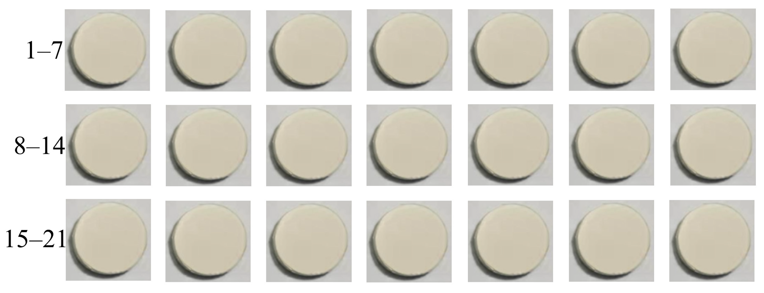
2.1. Experimental Sample Preparation

The experimental setup employed in this study was the same as that used in a previous study [3]. The adopted Fritillaria cirrhosa and Fritillaria thunbergii powder samples were purchased from Anhui Tong Huatang Chinese Herbal Beverage Technology Co. (Bozhou, China) and Sichuan Haorui Gallium Biotechnology Co. (Chengdu, China). In the experimental procedure, the powdered Fritillaria cirrhosa and Fritillaria thunbergii were first mixed into experimental samples with 21 different adulteration levels, as listed in Table 1. Subsequently, for each sample, the powdered samples were continuously and vigorously vibrated at 1000 rpm for 10 h using a multifunctional vortex mixer (VM-500Pro, Joanlab, Huzhou, China). Next, the powdered samples were retrieved, placed on weighing paper, and weighed with an electronic balance (BSA124S-CW, Sartorius, Shanghai, China); accordingly, a 0.5-g weight was obtained. The samples were then pressed for 5 min at a 20-MPa pressure using a tablet press (HY-12 Tianjin, Tianguang Optical Instruments Co., Ltd., Tianjin, China) to obtain disc shaped samples with a diameter and thickness of 13 and 2 mm, respectively, and each sample with different doping levels was pressed into two slices, as illustrated in Figure 1. Finally, the pressed samples were placed on a three-dimensional motorized translation table, and 100 LIBS spectra were obtained at different positions for each sample; accordingly, 200 spectra were obtained for two tablets of each sample, and then two spectra were averaged into one spectrum. Finally, 100 LIBS spectra were obtained for each experimental sample with a different doping level.
Table 1. Experimental samples of 21 different doping levels.
Figure 1. Physical diagram of the experimental samples with 21 different doping levels.

2.2. LIBS Experiments

The main LIBS setup of our experiments has been shown in the previous work [3]. A homemade Q-switched Nd: YAG laser (1064 nm, 30 mJ, 1 Hz, 10 ns) is used as the excitation source. The laser beam is reflected by three mirrors and then focused onto the sample surface with a NIR-corrected microscopic objective (Mitutoyo, 10X, working distance is 30.5 mm). The plasma radiation is collected and focused into a 600 μm fiber using convex lenses. Then, the LIBS spectra are analyzed by the fiber spectrometer (AvaSpec 2048-2-USB2, Avantes) with a range of 190~1100 nm and a resolution of 0.2~0.3 nm.

3. Results and Discussion

3.1. LIBS Spectra of the Samples

The typical LIBS spectra of 21 randomly selected experimental samples with different doping levels are presented in Figure S1. The Ca, Na, K, H, O, and N elements, including the CN and C2 molecular bands, were identified in the experimental samples and labelled in the LIBS spectra of Sample 1. From Figure S1, the intensities of H, O, N, CN, and C2 in the LIBS spectra of the experimental samples with different doping levels are independent of the doping amount of Fritillaria thunbergii, which is primarily influenced by air. To eliminate the interference of airborne components on the intensities of the LIBS spectra of the experimental samples, non-metallic elements were not used in subsequent analyses. The wavelength of 300–800 nm and intensities greater than 1000 counts of Ca (393.3 nm, 396.8 nm, and 422.6 nm), Na (588.9 nm and 589.5 nm), and K (766.4 nm and 769.8 nm) for three metallic elements are presented in Table 2 for the seven LIBS spectral lines.
Table 2. Three metal elements and their wavelengths in the experimental samples.

3.2. Quantitative Analysis Modelling

In this study, the data point intensities of seven spectral lines for each spectrum of three metal elements were adopted as input variables (66 variables in total), 100 LIBS spectra from each of Samples 4, 6, 8, 14, 16, and 18 were used as the test set, and 100 LIBS spectra from each of the remaining 15 samples were utilized as the training set to develop the PLSR model.

3.2.1. Data Standardization

Data normalization can reduce the fluctuations between the LIBS spectra of Fritillaria and improve the performance of quantitative analysis models. The effects of the MC, NA, SNV, and NM methods on the performance of the quantitative models were discussed. The mean absolute error (MAE) and RMSEP of the test set obtained using the PLSR model under the four data normalization methods are listed in Table 3.
Table 3. MAE and RMSEP of the test set obtained using the PLSR model under the four data normalization methods.
From Table 3, the MAE values of the test set obtained using the PLSR quantitative analysis model under the four data normalization methods of MC, NA, SNV, and NM are 24.2832%, 48.0711%, 8.6604%, and 8.6111%, respectively; the RMSEP values of the test set obtained are 26.6806%, 60.7073%, 10.8970%, and 10.8760%, respectively. Among the four data normalization methods, the MAE and RMSEP values of the PLSR model’s test set were the lowest by pre-processing the data using the NM method. The relationship between the predicted and standard values of the test set obtained by the PLSR quantitative analysis method under NM data normalization is illustrated in Figure 2; evidently, the MAE and RMSEP values of the test set are 8.6111% and 10.8760%, respectively, and the coefficient of determination, R2, of the test set’s fitted straight line is 0.9651. The error bars in Figure 3 represents the standard deviation (SD) of the predicted value based on measurements. We calculated the SD value of Equation (1) in all the figures of this work.
S = 1 n 1 i = 1 n ( x i x ¯ ) 2
where the x ¯ represent the average value of sample x i , i is the integer index, and n is the number of samples.
Figure 2. Plot of relationship between predicted and standard values of the test set obtained using the PLSR quantitative analysis method under NM data normalization.
Figure 3. Variance ratio of each PC and cumulative variance ratio.

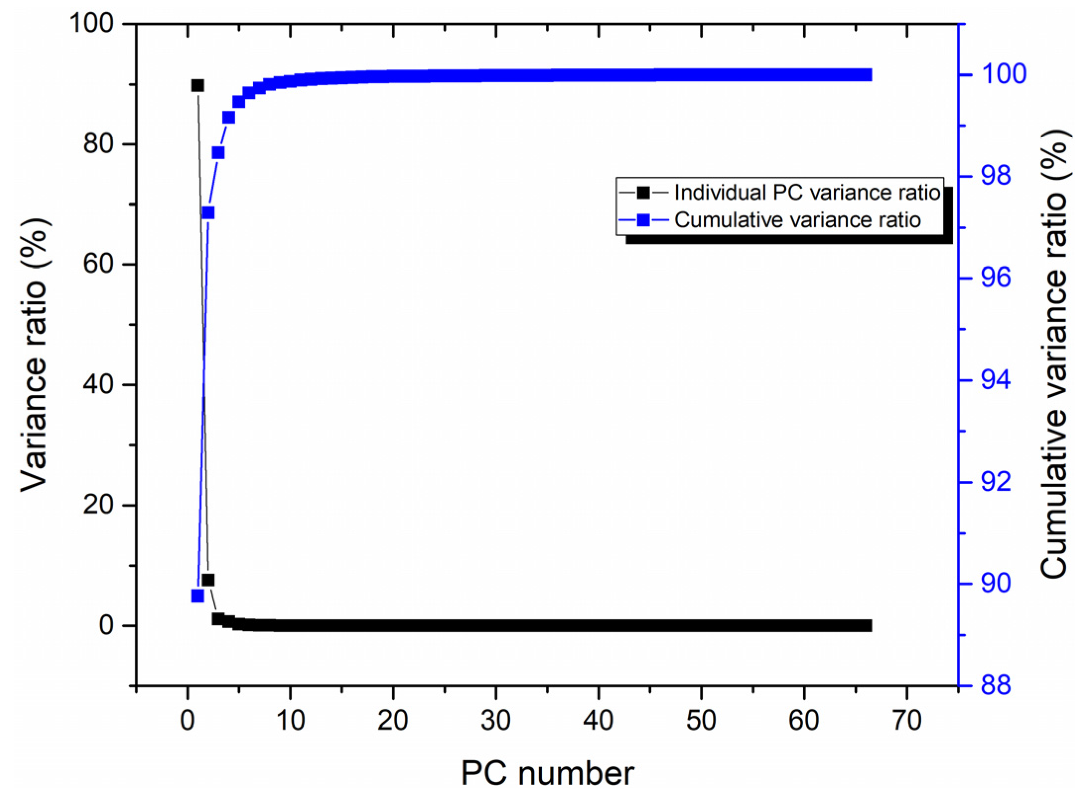
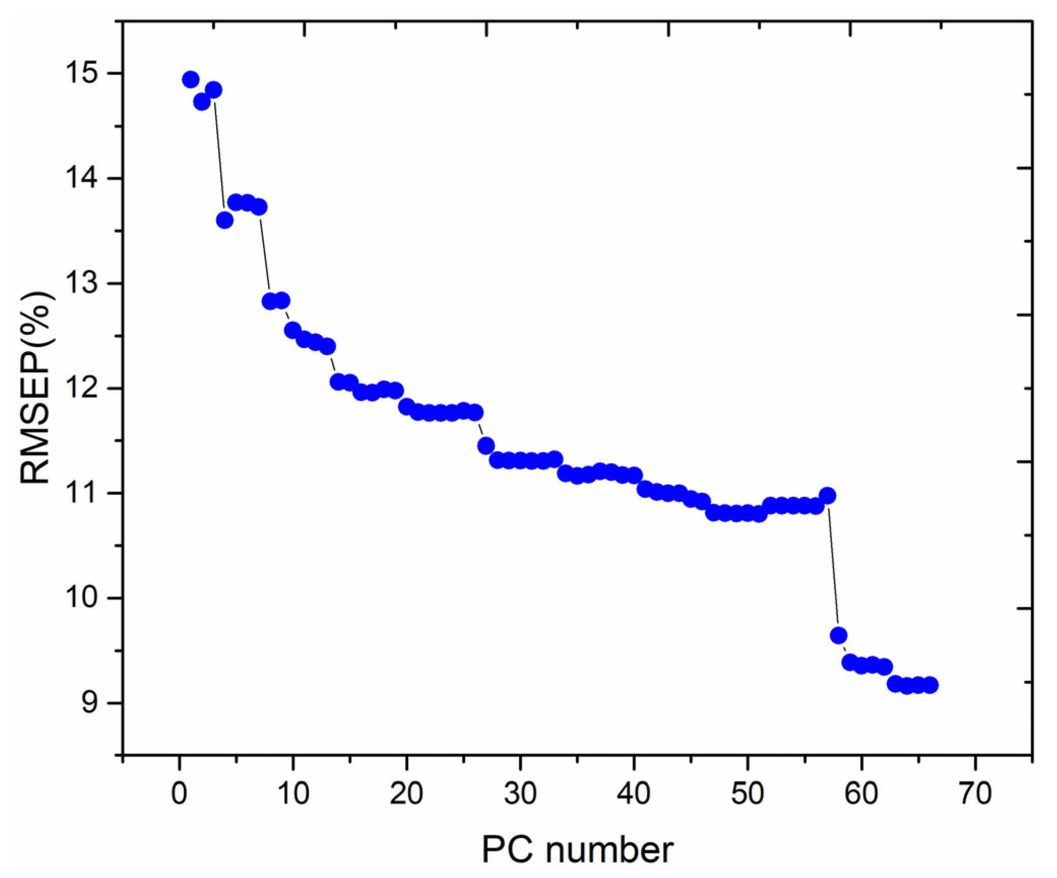
3.2.2. Feature Variable Selection

To reduce the amount of data input, discard noise and unimportant features, and to achieve the objective of improving the speed of data processing, it is necessary to select feature variables. Feature variable selection includes two types of feature extraction and feature selection. Additionally, in this study, we adopted PCA and LASSO for feature extraction and feature selection, respectively. LASSO is a compressed estimate. It obtains a more refined model by constructing a penalty function, so that it compresses some coefficients and sets some coefficients to zero. Therefore, Lasso retains the advantages of subset contraction, and it is an estimation of processing with compound linear data.
After normalizing the data via the NM method, the feature variables were extracted from the LIBS spectral data using the PCA method. Figure 3 presents the variance ratio of each principal component (PC) and the cumulative variance ratio obtained after the feature extraction using the PCA method.
As illustrated in Figure 3, the percentage of variance of each individual PC gradually decreased, and the percentage of cumulative variance gradually increased as the number PC increased. The variance ratios of the first three PCs were 89.77%, 7.53%, and 1.17%. The first PC contained most of the original information, and the cumulative variance ratio of the first three PCs reached 98.47%.
To investigate the effect of the number of PCs on the performance of the PLSR quantitative analysis model, the PC scores were adopted as the inputs to the PLSR model for modelling, and the relationship between the RMSEP of the training set and the number of PCs is illustrated in Figure 4.
Figure 4. Effect of the number of PCs on the performance of the PLSR quantitative analysis model.
From Figure 4, the RMSEP of the training set fluctuates with the increase in PC number, exhibiting a general decreasing trend. When the number of PC is 64, the lowest RMSEP value is obtained via the PLSR quantitative analysis model. Therefore, the first 64 PCs are chosen for the test set data analysis. The relationship between the predicted and standard values of the test set obtained by using the PLSR quantitative analysis method for the first 64 PCs as input data is illustrated in Figure 5. From Figure 5, the MAE and RMSEP values of the test set are 7.1585% and 9.1709%, respectively, and the coefficient of determination, R2, of the test set’s fitted straight line is 0.9920.
Figure 5. Plot of the relationship between the predicted and standard values of the test set obtained for the first 64 PCs as inputs to the PLSR model.
To investigate the effect on the performance of the PLSR model after adopting LASSO feature selection for quantitative analysis, the LIBS spectral data of the samples were first standardized using the NM method; subsequently, the importance of the data after standardizing the LIBS spectra was evaluated using the LASSO method, and the importance weight values of 66 variables were obtained. Finally, the importance weight values of the 66 variables were normalized, and the obtained normalized weight values based on the training set data are presented in Figure 6.
Figure 6. Normalized weight values of 66 variables obtained for the importance assessment of the LIBS spectral lines using the LASSO method.
Figure 6 shows the normalized weight values of 66 variables obtained for the importance assessment of the LIBS spectral lines using the LASSO method. Among the 66 spectral features, nine of them have normalized weight values of 0, thus indicating that these nine features do not play a role in the quantitative analysis. Meanwhile, the elements corresponding to the top 57 wavelengths in importance ranking, and their importance weights are listed in Table 4.
Table 4. Elements and importance weights corresponding to the top 57 wavelengths in importance ranking.
To investigate the effect of the number of features on the performance of the PLSR quantitative analysis model, the 57 spectral features with non-zero normalized weight values were ranked according to the normalized weight values from the largest to the smallest. The different numbers of spectral features, corresponding to the top 1–57 normalized weight values, were adopted as inputs to the PLSR model, respectively, and the relationship between the RMSEP of training set and the number of spectral features is illustrated in Figure 7.
Figure 7. Effect of the number of spectral features on the performance of the PLSR quantitative analysis model.
As illustrated in Figure 7, the RMSEP of the training set fluctuates with the increase in the number of spectral features, exhibiting a general decreasing trend. The RMSEP value obtained using the PLSR quantitative analysis model is lowest when the number of input spectral features is 57. Then, these 57 features are used in the test data analysis. The relationship between the predicted and standard values of the test set using the PLSR quantitative analysis model for the first 57 spectral features as input data is illustrated in Figure 8. From Figure 8, it can be seen that the MAE and RMSEP values of the test set are 7.1038% and 9.1523%, respectively, and the coefficient of determination, R2, of the test set’s fitted straight line is 0.9728.
Figure 8. Plot between the predicted and standard values of the test set for the first 57 spectral features as inputs to the PLSR model.
Compared with the PCA-PLSR model, the MAE and RMSEP of the predicted values of the LASSO-PLSR model’s test set were relatively better, decreasing from 7.1585% to 7.1038% and from 9.1709% to 9.1523%, respectively.

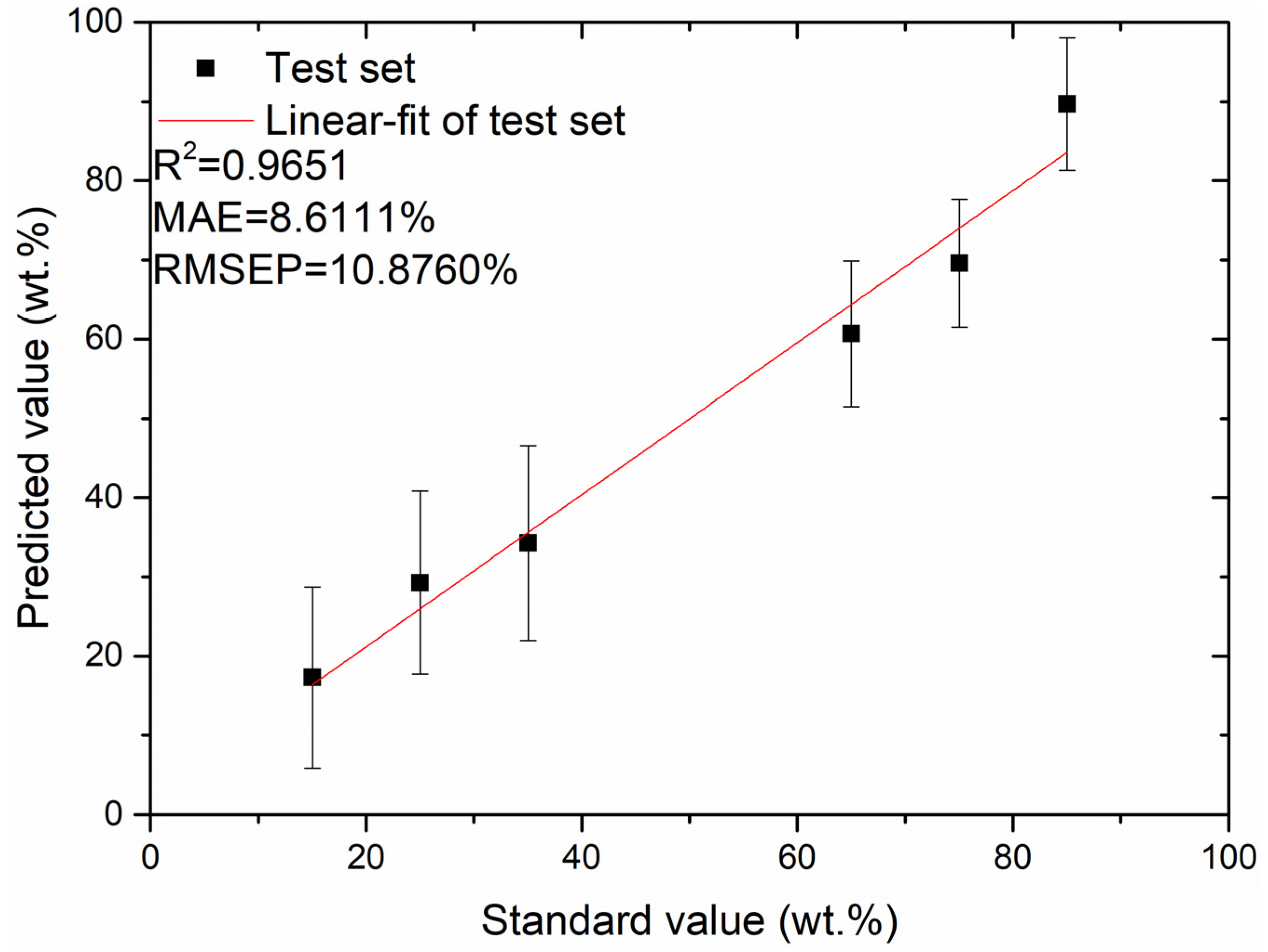
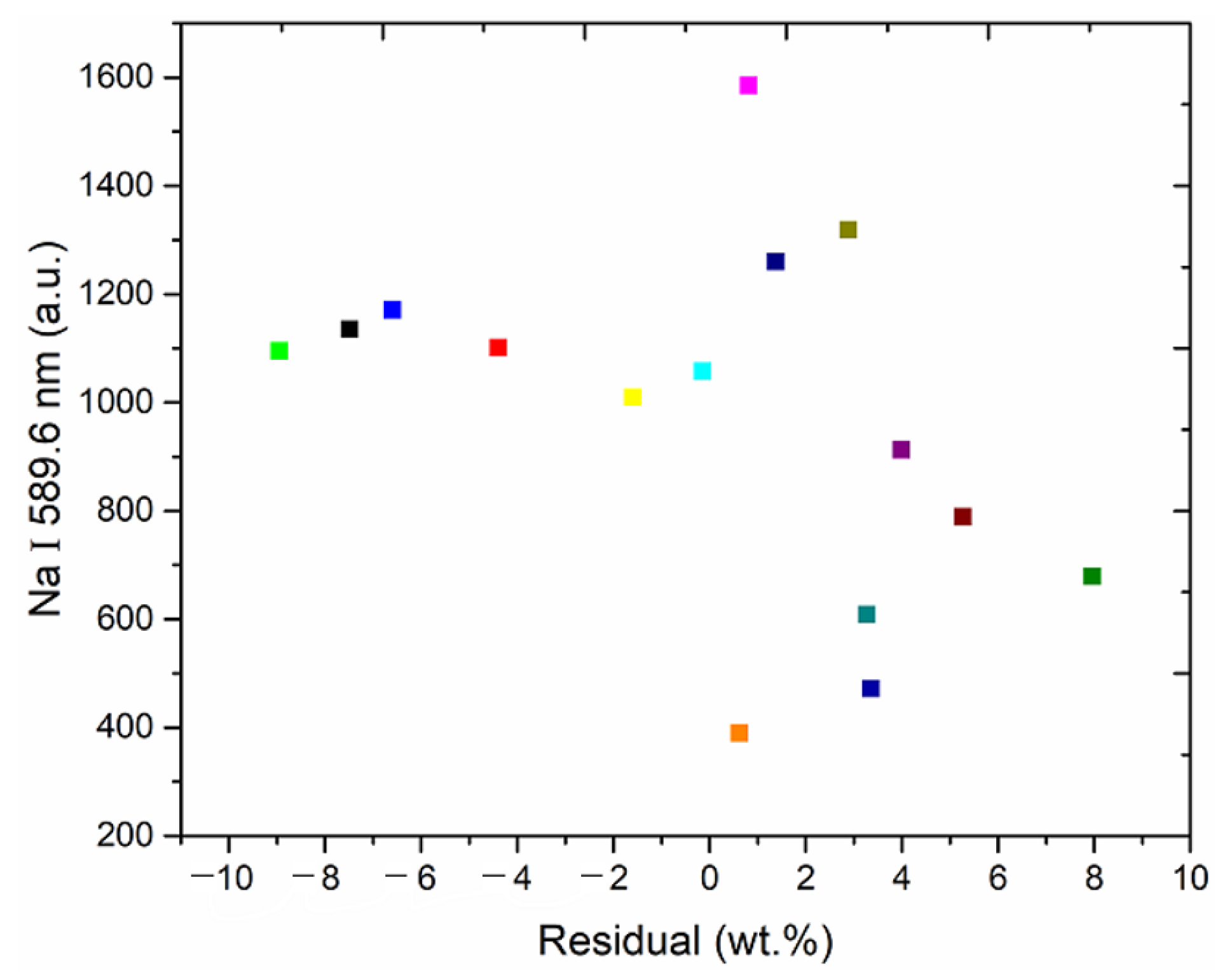
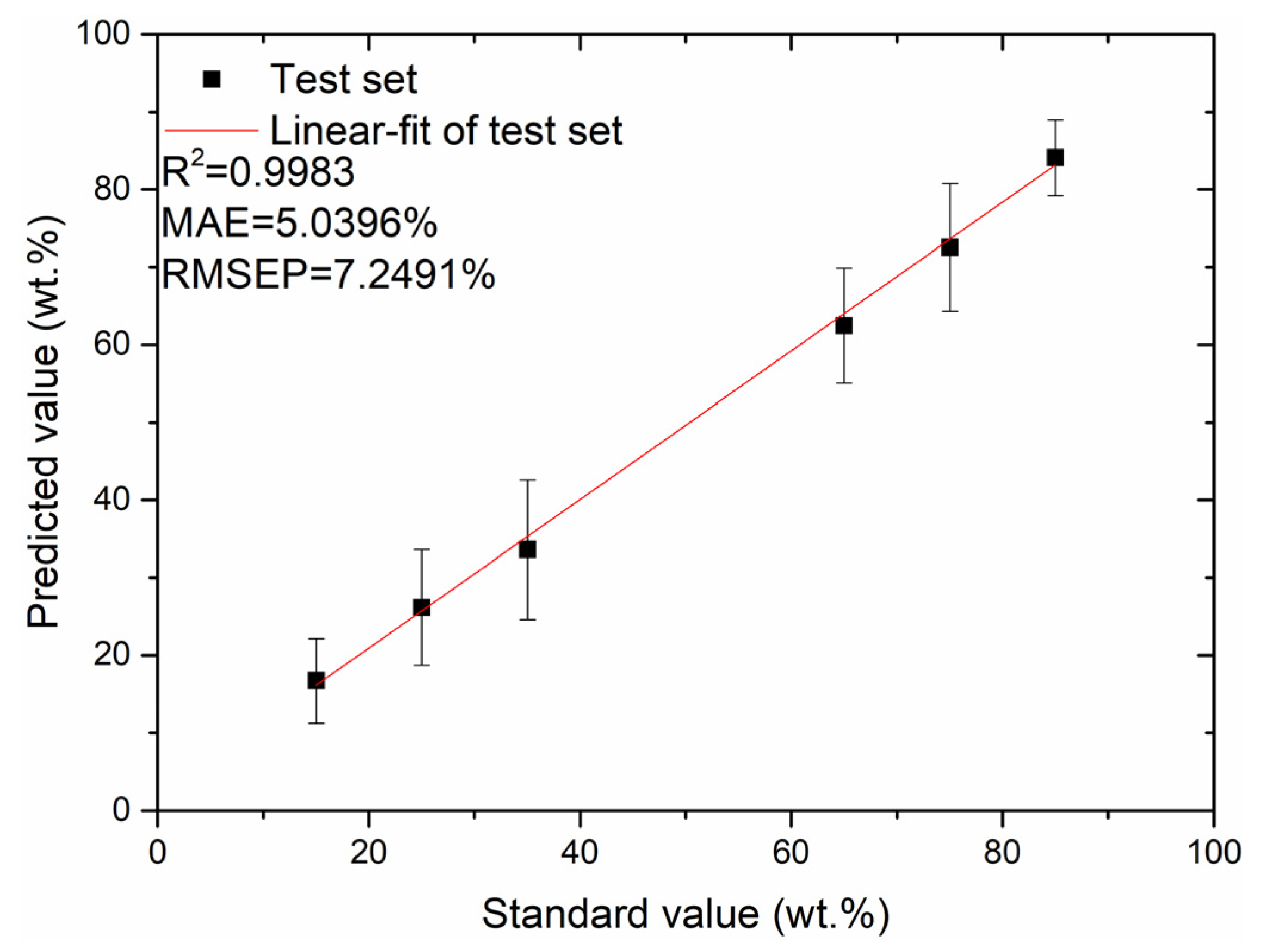
3.2.3. Residual Correction

The residual values were obtained by subtracting the predicted values of the LASSO-PLSR model from the standard values and were corrected using SVR. The SVR is a common kind of traditional machine learning method, which has extraordinary performance in the small sample training. In SVR, the straight line required for fitting data becomes a hyperplane. The SVR creates an “interval band” on both sides of the linear function, which does not calculate the loss for all samples falling into the interval zone. The samples outside the interval zone are recognized as support vectors. That is, only the support vector will affect its function model. Finally, the optimized model is obtained by minimizing total loss and maximum interval.
The relationship between the mean value of the residuals of the 100 spectra of each modelled sample and the mean value of the intensity of the most important spectral line (Na I 589.6 nm) is illustrated in Figure 9.
Figure 9. Plot of the average of the residuals of 100 spectra of each modelled sample against the average of the intensities of the most important spectral lines (Na I 589.6 nm).
As illustrated in Figure 9, the data points comprising the average of the residuals of 100 spectra of each modelled sample and the average of the intensity of the most important spectral line (Na I 589.6 nm) are randomly distributed and exhibit a nonlinear relationship overall. To further improve the accuracy of the quantitative analysis model, the most prevalent nonlinear kernel function in SVR (radial basis kernel function) was adopted to develop a SVR-based residual correction model with optimal parameters (c = 76.7312, g = 9.3966), and the predicted value of the PLSR model plus the predicted value of the SVR correction model was considered as the final predicted value. The relationship between the predicted and standard values of the test set, based on the LASSO-PLSR-SVR residual correction model, is illustrated in Figure 10; from this figure, it can be seen that the MAE and RMSEP values of the test set are 5.0396% and 7.2491%, respectively, and the coefficient of determination, R2, of the test set’s fitted straight line is 0.9983.
Figure 10. Plot of relationship between the predicted and standard values of the test set based on the LASSO-PLSR-SVR residual correction model.
From Figure 8 and Figure 10, it can be seen that the performance of the LASSO-PLSR-SVR residual correction-based model improved better than the LASSO-PLSR-based model in the quantitative analysis of the Fritillaria LIBS spectral data. The MAE value of the test set decreased from 7.1038% to 5.0396%, the RMSEP value decreased from 9.1523% to 7.2491%, and the coefficient of determination R2 of the test set’s fitted straight line increased from 0.9728 to 0.9983. The obtained results indicate that the residual correction model can compensate for the limitations of the conventional PLSR model in elucidating nonlinear characteristic variables and ultimately improve the prediction accuracy of the quantitative analysis model.

4. Conclusions

In this study, we proposed the adoption of the LIBS technique, combined with machine learning methods in the rapid test of adulteration levels in Fritillaria cirrhosa powder. Using PLSR as a quantitative analysis model, the effects of four data normalization methods, MC, NA, SNV, and NM, on the quantitative analysis performance of the PLSR model, were compared, among which the NM data normalization method exhibited the best performance. Accordingly, the effects of feature extraction and feature selection on the quantitative analysis performance of the PLSR model using PCA and LASSO were compared and analysed, and the performance of the LASSO-PLSR-based model was to be relatively better. A correction model for the residuals was further developed using SVR to compensate for the limitations of the conventional PLSR model in elucidating the nonlinear feature variables. The final LASSO-PLSR-SVR-based residual correction model improved the accuracy of the quantitative analysis relative to the LASSO-PLSR model, and the MAE of the test set decreased from 7.1038% to 5.0396%, the RMSEP decreased from 9.1523% to 7.2491%, and the coefficient of determination R2 of the test set’s fitted straight line increased from 0.9782 to 0.9983. The experimental results demonstrated the effectiveness of adopting the LIBS technique combined with machine learning in the rapid test of adulteration levels in Fritillaria cirrhosa powder. Furthermore, this study has important application value for drug testing, regulation, and quality control.

Supplementary Materials

The following supporting information can be downloaded at: https://www.mdpi.com/article/10.3390/foods12081710/s1, Figure S1. Typical LIBS spectra of 21 experimental samples with different doping levels.

Author Contributions

Conceptualization, Software and Writing—original draft, K.W.; Supervision, Funding acquisition, Q.W.; Methodology, G.T. and X.X.; Investigation, Z.Z. and H.L.; Validation, M.B. and Y.Z.; Resources, T.L. and B.L. All authors have read and agreed to the published version of the manuscript.

Funding

This research was funded by the National Natural Science Foundation of China (No. 62075011).

Institutional Review Board Statement

Not applicable.

Data Availability Statement

Data is contained within the article or supplementary material.

Conflicts of Interest

The authors declare no conflict of interest.

References

  1. Jiang, R.P.; Zou, M.; Qin, Y.; Tan, G.D.; Huang, S.P.; Quan, H.G.; Zhou, J.Y.; Liao, H. Modeling of the potential geographical distribution of three Fritillaria species under climate change. Front. Plant Sci. 2022, 12, 749838. [Google Scholar] [CrossRef] [PubMed]
  2. Lu, Q.X.; Li, R.; Liao, J.Q.; Hu, Y.Q.; Gao, Y.D.; Wang, M.C.; Li, J.; Zhao, Q. Integrative analysis of the steroidal alkaloids distribution and biosynthesis of Bulbus Fritillariae cirrhosae through metabolome and transcriptome analyses. BMC Genom. 2022, 23, 511. [Google Scholar] [CrossRef] [PubMed]
  3. Wei, K.; Cui, X.T.; Teng, G.E.; Khan, M.N.; Wang, Q.Q. Distinguish Fritillaria cirrhosa and non-Fritillaria cirrhosa using laser-induced breakdown spectroscopy. Plasma Sci. Technol. 2021, 23, 085507. [Google Scholar] [CrossRef]
  4. Hu, G.L.; Chen, R.Z.; Cheng, K.; Lv, X.Y. Rapid quantitative determination of Fritillaria thunbergia miq mixed into Fritillaria cirrhosa D. don by near-infrared diffuse reflectance spectroscopy. Chin. J. Pharm. Anal. 2005, 25, 150–152. [Google Scholar]
  5. Shen, T.T.; Li, W.J.; Zhang, X.; Kong, W.W.; Liu, F.; Wang, W.; Peng, J.Y. High-sensitivity determination of nutrient elements in panax notoginseng by laser-induced breakdown spectroscopy and chemometric methods. Molecules 2019, 24, 1525. [Google Scholar] [CrossRef] [PubMed]
  6. Wei, K.; Wang, Q.Q.; Teng, G.E.; Xu, X.J.; Zhao, Z.F.; Chen, G.Y. Application of laser-induced breakdown spectroscopy combined with chemometrics for identification of penicillin manufacturers. Appl. Sci. 2022, 12, 4981. [Google Scholar] [CrossRef]
  7. Wang, Q.Q.; Cui, X.T.; Teng, G.E.; Zhao, Y.; Wei, K. Evaluation and improvement of model robustness for plastics samples classification by laser-induced breakdown spectroscopy. Opt. Laser Technol. 2020, 125, 106035. [Google Scholar] [CrossRef]
  8. Cui, X.T.; Wang, Q.Q.; Wei, K.; Teng, G.E.; Xu, X.J. Laser-induced breakdown spectroscopy for the classification of wood materials using machine learning methods combined with feature selection. Plasma Sci. Technol. 2021, 23, 055505. [Google Scholar] [CrossRef]
  9. Khan, M.N.; Wang, Q.Q.; Idrees, B.S.; Xiangli, W.T.; Teng, G.E.; Cui, X.T.; Zhao, Z.F.; Wei, K.; Abrar, M. A review on laser-induced breakdown spectroscopy in different cancers diagnosis and classification. Front. Phys. 2022, 10, 821057. [Google Scholar] [CrossRef]
  10. Wang, Q.Q.; Xiangli, W.T.; Teng, G.E.; Cui, X.T.; Wei, K. A brief review of laser-induced breakdown spectroscopy for human and animal soft tissues: Pathological diagnosis and physiological detection. Appl. Spectrosc. Rev. 2021, 56, 221–241. [Google Scholar] [CrossRef]
  11. Han, J.H.; Moon, Y.; Lee, J.J.; Choi, S.; Kim, Y.; Jeong, S. Differentiation of cutaneous melanoma from surrounding skin using laser-induced breakdown spectroscopy. Biomed. Opt. Express 2016, 7, 57–65. [Google Scholar] [CrossRef] [PubMed]
  12. Ahmadi, S.H.; Keshavarz, M.H.; Atabak, H.R.H. Introducing laser induced breakdown spectroscopy (LIBS) as a novel, cheap and non-destructive method to study the changes of mechanical properties of plastic bonded explosives (PBX). Z. Anorg. Allg. Chem. 2018, 644, 1667–1673. [Google Scholar] [CrossRef]
  13. Shaik, A.K.; Epuru, N.R.; Syed, H.; Byram, C.; Soma, V.R. Femtosecond laser induced breakdown spectroscopy based standoff detection of explosives and discrimination using principal component analysis. Opt. Express 2018, 26, 8069–8083. [Google Scholar] [CrossRef] [PubMed]
  14. Zhang, W.; Tang, Y.; Shi, A.R.; Bao, L.R.; Shen, Y.; Shen, R.Q.; Ye, Y.H. Recent developments in spectroscopic techniques for the detection of explosives. Materials 2018, 11, 1364. [Google Scholar] [CrossRef] [PubMed]
  15. Sheta, S.; Afgan, M.S.; Hou, Z.Y.; Yao, S.C.; Zhang, L.; Li, Z.; Wang, Z. Coal analysis by laser-induced breakdown spectroscopy: A tutorial review. J. Anal. Atom. Spectrom. 2019, 34, 1047–1082. [Google Scholar] [CrossRef]
  16. Liu, C.; Luo, Y.M.; Zhang, Q.Z. Laser-induced breakdown spectroscopy-based coal-rock recognition: An in situ sampling and recognition method. IEEE Access 2021, 9, 164732–164741. [Google Scholar] [CrossRef]
  17. Dong, M.R.; Wei, L.P.; Gonzalez, J.J.; Oropeza, D.; Chirinos, J.; Mao, X.L.; Lu, J.D.; Russo, R.E. Coal discrimination analysis using tandem laser-induced breakdown spectroscopy and laser ablation inductively coupled plasma time-of-flight mass spectrometry. Anal. Chem. 2020, 92, 7003–7010. [Google Scholar] [CrossRef]
  18. Liu, K.; Tian, D.; Li, C.; Li, Y.C.; Yang, G.; Ding, Y. A review of laser-induced breakdown spectroscopy for plastic analysis. TrAC-Trend. Anal. Chem. 2019, 110, 327–334. [Google Scholar] [CrossRef]
  19. Junjuri, R.; Zhang, C.; Barman, I.; Gundawar, M.K. Identification of post-consumer plastics using laser-induced breakdown spectroscopy. Polym. Test. 2019, 76, 101–108. [Google Scholar] [CrossRef]
  20. Peng, X.Y.; Xu, B.H.; Xu, Z.Y.; Yan, X.T.; Zhang, N.; Qin, Y.Z.; Ma, Q.X.; Li, J.M.; Zhao, N.; Zhang, Q.M. Accuracy improvement in plastics classification by laser-induced breakdown spectroscopy based on a residual network. Opt. Express 2021, 29, 33269–33280. [Google Scholar] [CrossRef]
  21. Markiewicz-Keszycka, M.; Cama-Moncunill, X.; Casado-Gavalda, M.P.; Dixit, Y.; Cama-Moncunill, R.; Cullen, P.J.; Sullivan, C. Laser-induced breakdown spectroscopy (LIBS) for food analysis: A review. Trends Food Sci. Tech. 2017, 65, 80–93. [Google Scholar] [CrossRef]
  22. Senesi, G.S.; Cabral, J.; Menegatti, C.R.; Marangoni, B.; Nicolodelli, G. Recent advances and future trends in LIBS applications to agricultural materials and their food derivatives: An overview of developments in the last decade (2010–2019). Part II. Crop plants and their food derivatives. TrAC-Trend. Anal. Chem. 2019, 118, 453–469. [Google Scholar] [CrossRef]
  23. Velasquez-Ferrin, A.; Babos, D.V.; Marina-Montes, C.; Anzano, J. Rapidly growing trends in laser-induced breakdown spectroscopy for food analysis. Appl. Spectrosc. Rev. 2021, 56, 492–512. [Google Scholar] [CrossRef]
  24. Lin, X.M.; Li, H.; Yao, Q.H. Signal detection of carbon in iron-based alloy by double-pulse laser-induced breakdown spectroscopy. Plasma Sci. Technol. 2015, 17, 953–957. [Google Scholar] [CrossRef]
  25. Qi, L.F.; Sun, L.X.; Xin, Y.; Cong, Z.B.; Li, Y.; Yu, H.B. Application of stand-off double-pulse laser-induced breakdown spectroscopy in elemental analysis of magnesium alloy. Plasma Sci. Technol. 2015, 17, 676–681. [Google Scholar] [CrossRef]
  26. Aberkane, S.M.; Abdelhamid, M.; Mokdad, F.; Yahiaoui, K.; Abdelli-Messaci, S.; Harith, M.A. Sorting zamak alloys via chemometric analysis of their LIBS spectra. Anal. Methods 2017, 9, 3696–3703. [Google Scholar] [CrossRef]
  27. Yang, Y.W.; Hao, X.J.; Zhang, L.L.; Ren, L. Application of scikit and keras libraries for the classification of iron ore data acquired by laser-induced breakdown spectroscopy (LIBS). Sensors 2020, 20, 1393. [Google Scholar] [CrossRef]
  28. Sheng, L.W.; Zhang, T.L.; Niu, G.H.; Wang, K.; Tang, H.S.; Duan, Y.X.; Li, H. Classification of iron ores by laser-induced breakdown spectroscopy (LIBS) combined with random forest (RF). J. Anal. Atom. Spectrom. 2015, 30, 453–458. [Google Scholar] [CrossRef]
  29. Wang, P.; Li, N.; Yan, C.H.; Feng, Y.Z.; Ding, Y.; Zhang, T.L.; Li, H. Rapid quantitative analysis of the acidity of iron ore by the laser-induced breakdown spectroscopy (LIBS) technique coupled with variable importance measures-random forests (VIM-RF). Anal. Methods 2019, 11, 3419–3428. [Google Scholar] [CrossRef]
  30. Villas-Boas, P.R.; Franco, M.A.; Martin-Neto, L.; Gollany, H.T.; Milori, D.M.B.P. Applications of laser-induced breakdown spectroscopy for soil analysis, part I: Review of fundamentals and chemical and physical properties. Eur. J. Soil Sci. 2020, 71, 789–804. [Google Scholar] [CrossRef]
  31. Yi, R.X.; Li, J.M.; Yang, X.Y.; Zhou, R.; Yu, H.W.; Hao, Z.Q.; Guo, L.B.; Li, X.Y.; Zeng, X.Y.; Lu, Y.F. Spectral interference elimination in soil analysis using laser-induced breakdown spectroscopy assisted by laser-induced fluorescence. Anal. Chem. 2017, 89, 2334–2337. [Google Scholar] [CrossRef] [PubMed]
  32. Gazeli, O.; Stefas, D.; Couris, S. Sulfur detection in soil by laser induced breakdown spectroscopy assisted by multivariate analysis. Materials 2021, 14, 541. [Google Scholar] [CrossRef] [PubMed]
  33. Liu, X.N.; Ma, Q.; Liu, S.S.; Shi, X.Y.; Zhang, Q.; Wu, Z.S.; Qiao, Y.J. Monitoring As and Hg variation in An-Gong-Niu-Huang Wan (AGNH) intermediates in a pilot scale blending process using laser-induced breakdown spectroscopy. Spectrochim. Acta A 2015, 151, 547–552. [Google Scholar] [CrossRef] [PubMed]
  34. Zhu, C.W.; Lv, J.X.; Liu, K.; Li, Q.Z.; Tang, Z.Y.; Zhou, R.; Zhang, W.; Chen, J.; Liu, K.; Li, X.Y.; et al. Fast detection of harmful trace elements in glycyrrhiza using standard addition and internal standard method-Laser-induced breakdown spectroscopy (SAIS-LIBS). Microchem. J. 2021, 168, 106408. [Google Scholar] [CrossRef]
  35. Wang, J.M.; Xue, S.W.; Zheng, P.C.; Chen, Y.Y.; Peng, R. Determination of lead and copper in ligusticum wallichii by laser-induced breakdown spectroscopy. Anal. Lett. 2017, 50, 2000–2011. [Google Scholar] [CrossRef]
  36. Han, W.W.; Su, M.G.; Sun, D.X.; Yin, Y.P.; Wang, Y.P.; Gao, C.L.; Yang, F.C.; Fu, Y.B. Analysis of metallic elements dissolution in the astragalus at different decocting time by using LIBS technique. Plasma Sci. Technol. 2020, 22, 085501. [Google Scholar] [CrossRef]
  37. Nisar, S.; Dastgeer, G.; Shafiq, M.; Usman, M. Qualitative and semi-quantitative analysis of health-care pharmaceutical products using laser-induced breakdown spectroscopy. J. Pharm. Anal. 2019, 9, 20–24. [Google Scholar] [CrossRef]
  38. Iqbal, J.; Asghar, H.; Shah, S.K.H.; Naeem, M.; Abbasi, S.A.; Ali, R. Elemental analysis of sage (herb) using calibration-free laser-induced breakdown spectroscopy. Appl. Opt. 2020, 59, 4927–4932. [Google Scholar] [CrossRef]
  39. Hao, N.; Gao, X.; Zhao, Q.; Miao, P.Q.; Cheng, J.W.; Li, Z.; Liu, C.Q.; Li, W.L. Rapid origin identification of chrysanthemum morifolium using laser-induced breakdown spectroscopy and chemometrics. Postharvest Biol. Tec. 2023, 197, 112226. [Google Scholar] [CrossRef]
  40. Zhao, Q.; Yu, Y.; Cui, P.D.; Hao, N.; Liu, C.Q.; Miao, P.Q.; Li, Z. Laser-induced breakdown spectroscopy (LIBS) for the detection of exogenous contamination of metal elements in lily bulbs. Spectrochim. Acta B 2023, 287, 122053. [Google Scholar] [CrossRef]
Disclaimer/Publisher’s Note: The statements, opinions and data contained in all publications are solely those of the individual author(s) and contributor(s) and not of MDPI and/or the editor(s). MDPI and/or the editor(s) disclaim responsibility for any injury to people or property resulting from any ideas, methods, instructions or products referred to in the content.

Article Metrics

Citations

Article Access Statistics

Multiple requests from the same IP address are counted as one view.