
Coffee Yield Stability as a Factor of Food Security


Abstract
1. Introduction
2. Materials and Methods
3. Results
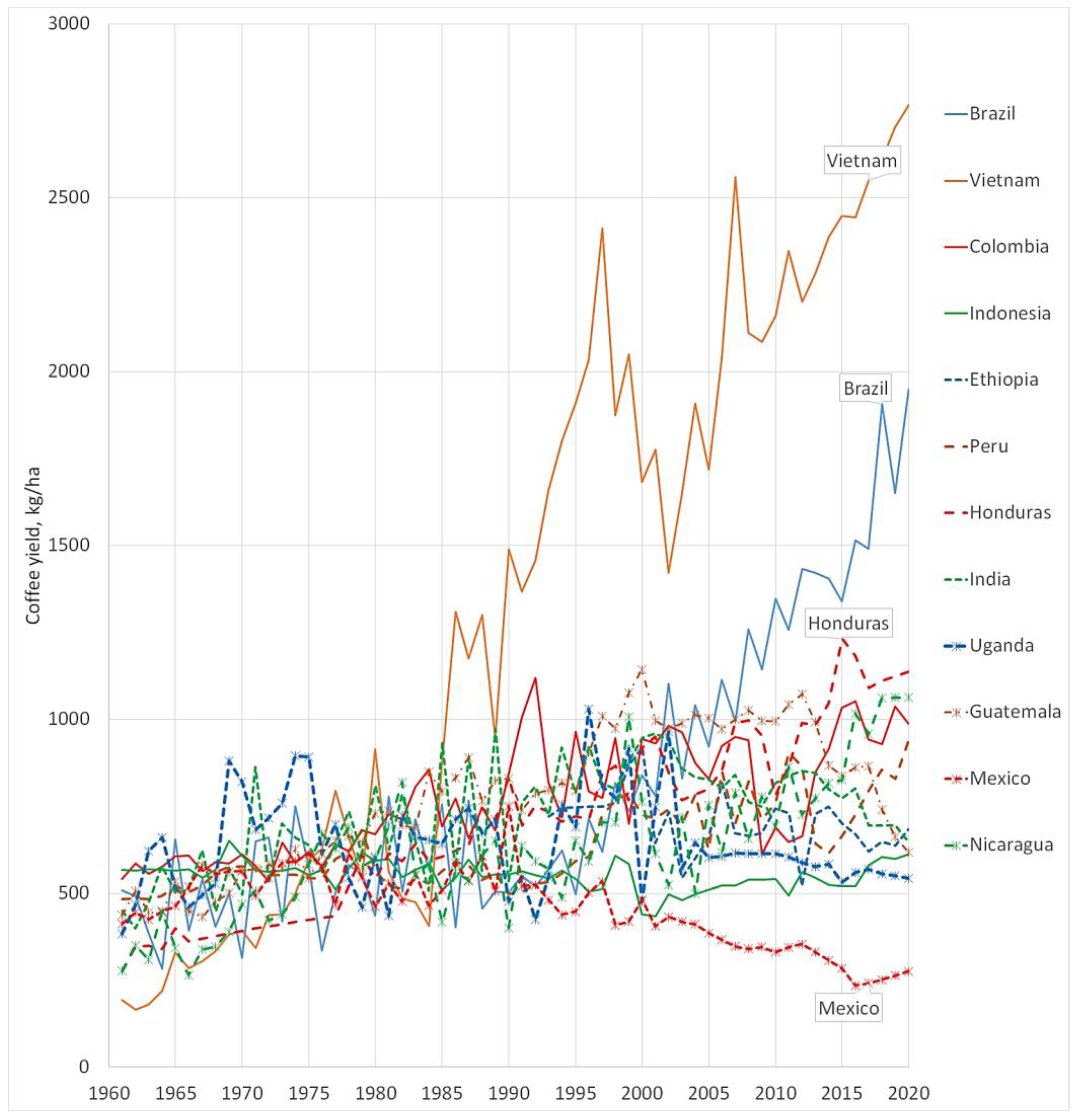
3.1. Yield Time Series, 1961–2020
3.2. Separate Analysis of the Time Periods 1961–1994 and 1995–2020
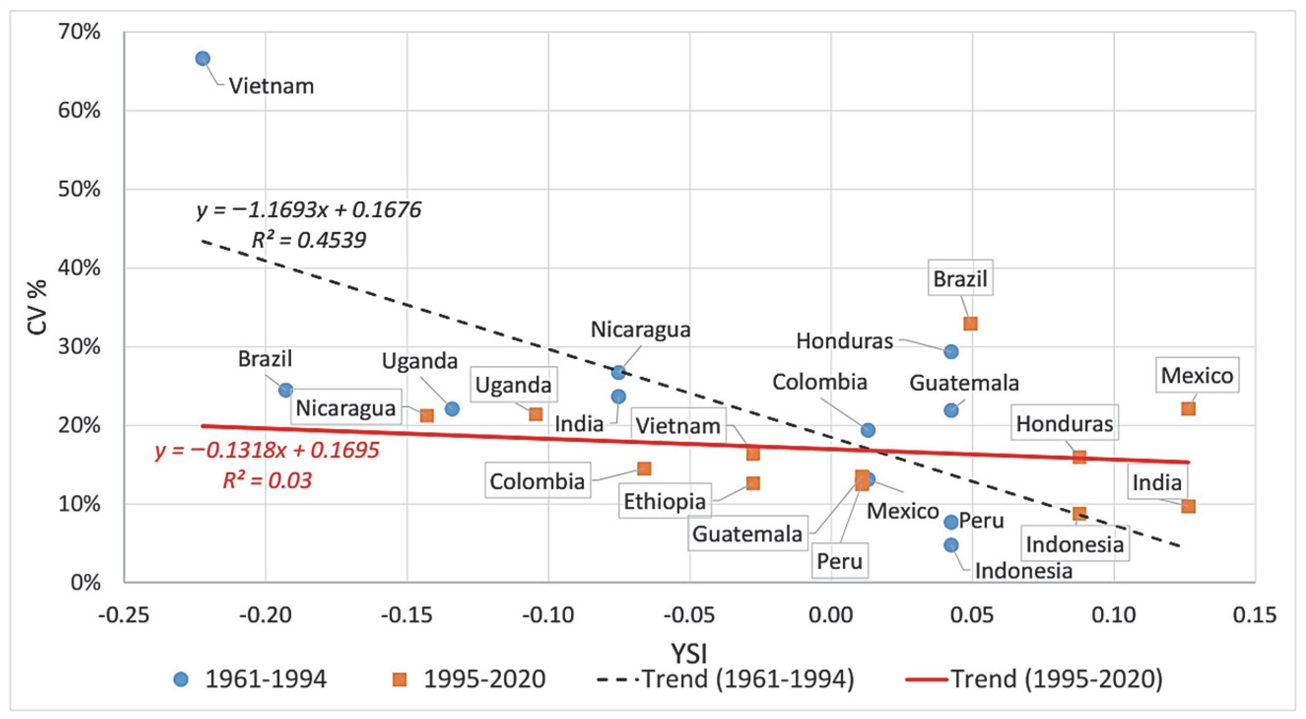
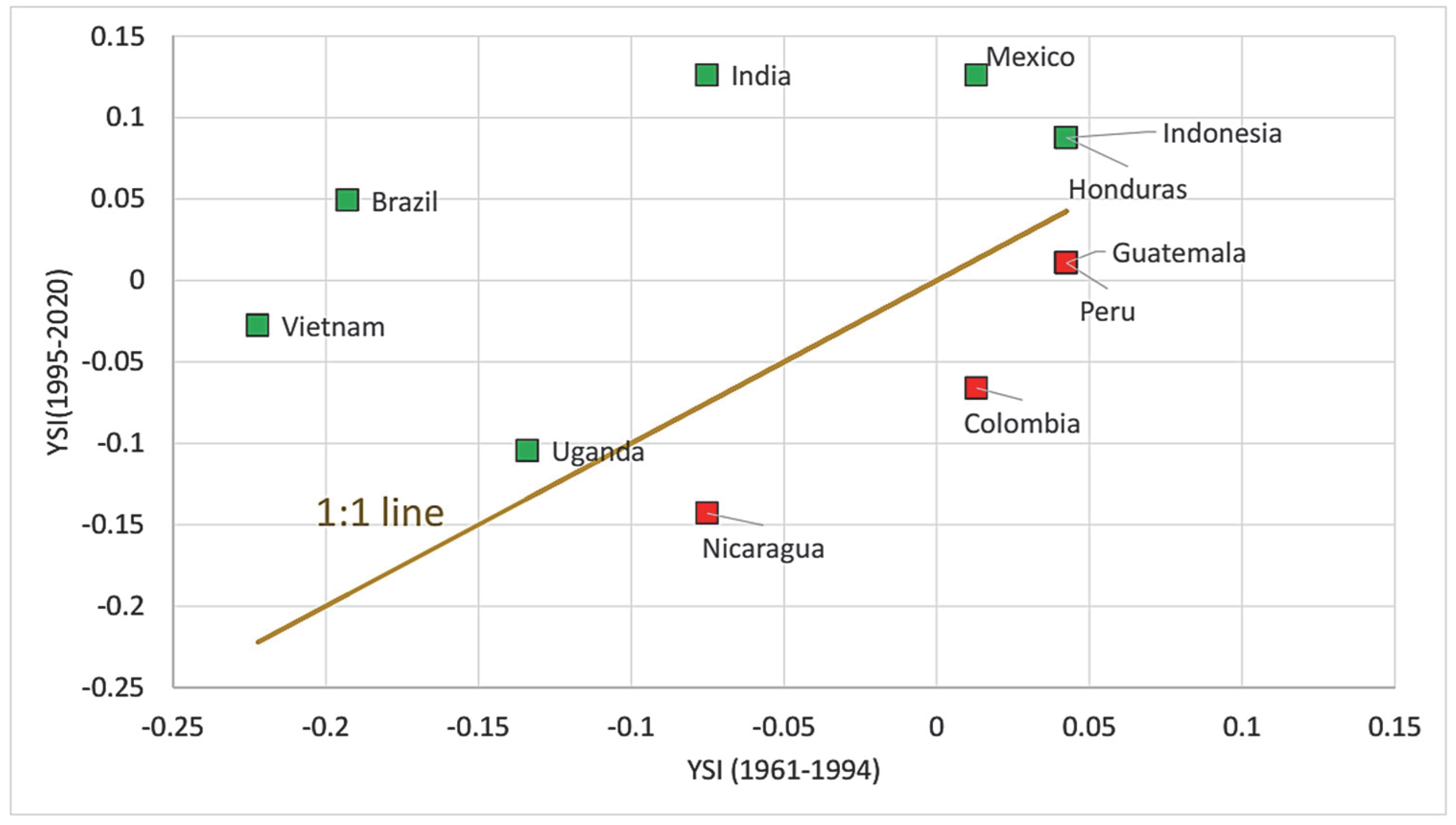
3.3. Comparison of Yield Volatilities during 1961–1994 and 1995–2020
4. Discussion
5. Conclusions
Author Contributions
Funding
Data Availability Statement
Acknowledgments
Conflicts of Interest
References
- UN. Transforming Our World: The 2030 Agenda for Sustainable Development; United Nations: San Francisco, CA, USA, 2015; Available online: https://sdg.un.org/goals (accessed on 10 July 2022).
- Abildtrup, J.; Audsley, E.; Fekete-Farkas, M.; Giupponi, C.; Gylling, M.; Rosato, P.; Rounsevell, M. Socio-economic scenario development for the assessment of climate change impacts on agricultural land use: A pairwise comparison approach. Environ. Sci. Policy 2006, 9, 101–115. [Google Scholar] [CrossRef]
- Winkler, K.; Fuchs, R.; Rounsevell, M.; Herold, M. Global land use changes are four times greater than previously estimated. Nat. Commun. 2021, 12, 2501. [Google Scholar] [CrossRef] [PubMed]
- Fróna, D.; Szenderák, J.; Harangi-Rákos, M. Economic effects of climate change on global agricultural production. Nat. Conserv. 2021, 44, 117–139. [Google Scholar] [CrossRef]
- Fróna, D.; Szenderák, J.; Harangi-Rákos, M. The Challenge of Feeding the World. Sustainability 2019, 11, 5816. [Google Scholar] [CrossRef]
- Batmunkh, A.; Nugroho, A.D.; Fekete-Farkas, M.; Lakner, Z. Global Challenges and Responses: Agriculture, Economic Globalization, and Environmental Sustainability in Central Asia. Sustainability 2022, 14, 2455. [Google Scholar] [CrossRef]
- Ali, S.; Ghosh, B.C.; Osmani, A.G.; Hossain, E.; Fogarassy, C. Farmers’ Climate Change Adaptation Strategies for Reducing the Risk of Rice Production: Evidence from Rajshahi District in Bangladesh. Agronomy 2021, 11, 600. [Google Scholar] [CrossRef]
- Pícha, K.; Skořepa, L. Preference to Food with a Regional Brand. Qual. Access Success 2018, 19, 134–139. Available online: https://www.calitatea.ro/assets/arhiva/2018/QAS_Vol.19_No.162_February-2018.pdf (accessed on 1 July 2022).
- ITC. The Coffee Guide; International Trade Centre: Geneva, Switzerland, 2021; Available online: https://intracen.org/media/file/5718 (accessed on 19 April 2022).
- Nicholson, C.F.; Stephens, E.C.; Kopainsky, B.; Jones, A.D.; Parsons, D.; Garrett, J. Food security outcomes in agricultural systems models: Current status and recommended improvements. Agric. Syst. 2021, 188, 103028. [Google Scholar] [CrossRef]
- Caswell, M.; Méndez, V.E.; Bacon, C.M. Food Security and Smallholder Coffee Production: Current Issues and Future Directions; RLG Policy Brief #1; Agroecology and Rural Livelihoods Group (ARLG), University of Vermont: Burlington, VT, USA, 2012; Available online: http://www.uvm.edu/~agroecol/?Page=Publications.html (accessed on 10 September 2022).
- Unnevehr, L. Food safety in developing countries: Moving beyond exports. Glob. Food Secur. 2015, 4, 24–29. [Google Scholar] [CrossRef]
- Chiputwa, B.; Spielman, D.J.; Qaim, M. Food Standards, Certification, and Poverty among Coffee Farmers in Uganda. World Development 2015, 66, 400–412. [Google Scholar] [CrossRef]
- Bacsi, Z.; Hollósy, Z. The Yield Stability Index Reloaded—The Assessment of the Stability of Crop Production Technology. Agric. Conspec. Sci. 2019, 84, 319–331. [Google Scholar]
- ICO. ICO Indicator Prices; International Coffee Organization: London, UK, 2022; Available online: https://ico.org/coffee_prices.asp (accessed on 9 August 2022).
- Castellana, F.; De Nucci, S.; De Pergola, G.; Di Chito, M.; Lisco, G.; Triggiani, V.; Sardone, R.; Zupo, R. Trends in Coffee and Tea Consumption during the COVID-19 Pandemic. Foods 2021, 10, 2458. [Google Scholar] [CrossRef] [PubMed]
- Williams, S.D.; Barkla, B.J.; Rose, T.J.; Liu, L. Does Coffee Have Terroir and How Should It Be Assessed? Foods 2022, 11, 1907. [Google Scholar] [CrossRef]
- Bastian, F.; Hutabarat, O.S.; Dirpan, A.; Nainu, F.; Harapan, H.; Emran, T.B.; Simal-Gandara, J. From Plantation to Cup: Changes in Bioactive Compounds during Coffee Processing. Foods 2021, 10, 2827. [Google Scholar] [CrossRef] [PubMed]
- Blumenthal, P.; Steger, M.C.; Quintanilla Bellucci, A.; Segatz, V.; Rieke-Zapp, J.; Sommerfeld, K.; Schwarz, S.; Einfalt, D.; Lachenmeier, D.W. Production of Coffee Cherry Spirits from Coffea arabica Varieties. Foods 2022, 11, 1672. [Google Scholar] [CrossRef] [PubMed]
- Läderach, P.; Ramirez–Villegas, J.; Navarro-Racines, C.; Zelaya, C.; Martinez–Valle, A.; Jarvis, A. Climate change adaptation of coffee production in space and time. Clim. Chang. 2017, 141, 47–62. [Google Scholar] [CrossRef]
- Sujatmiko, T.; Ihsaniyati, H. Implication of climate change on coffee farmers’ welfare in Indonesia. IOP Conf. Ser. Earth Environ. Sci. 2018, 200, 012054. [Google Scholar] [CrossRef]
- Ovalle-Rivera, O.; Läderach, P.; Bunn, C.; Obersteiner, M.; Schroth, G. Projected Shifts in Coffea arabica Suitability among Major Global Producing Regions Due to Climate Change. PLoS ONE 2015, 10, e0124155. [Google Scholar] [CrossRef]
- Grüter, R.; Trachsel, T.; Laube, P.; Jaisli, I. Expected global suitability of coffee, cashew and avocado due to climate change. PLoS ONE 2022, 17, e0261976. [Google Scholar] [CrossRef]
- FAO-TCL. FAOSTAT Database, Trade Indicators. 2022. Available online: https://www.fao.org/faostat/en/#data/TCL (accessed on 1 June 2022).
- Vargas, R.; Fonseca, C.; Hareau, G.; Ordinola, M.; Pradel, W.; Robiglio, V.; Suarez, V. Health crisis and quarantine measures in Peru: Effects on livelihoods of coffee and potato farmers. Agric. Syst. 2021, 187, 103033. [Google Scholar] [CrossRef]
- FAO-FS. FAOSTAT Suite of Food Security Indicators. 2022. Available online: https://www.fao.org/faostat/en/#data/FS. (accessed on 1 June 2022).
- Kovářová, K.; Nádeník, M.; Pícha, K. The Czech Republik Sugar Market Development in the Context of the Phasing Out of Sugar Quota. Deturope 2017, 9, 110–117. [Google Scholar] [CrossRef]
- Kovářová, K.; Procházková, K. Influence of the seasonal progress of the quality characteristics on the purchase prices of milk in context of the market situation (Vlív sezónní dynamiky jakostních ukazatelcú na vykupní cenu méka v kontextu situace na trhu.). Deturope 2017, 9, 35–46. [Google Scholar] [CrossRef]
- Heinemann, J.A.; Massaro, M.; Coray, D.S.; Zanon Agapito-Tenfen, S.; Wen, J.D. Sustainability and innovation in staple crop production in the US Midwest. Int. J. Agric. Sustain. 2014, 12, 71–88. [Google Scholar] [CrossRef]
- Takács-György, K.; Takács, I. Changes in cereal land use and production level in the European Union during the period 1999–2009, focusing on New Member States. Stud. Agric. Econ. 2012, 114, 24–30. Available online: https://studies.hu/wp-content/uploads/2019/05/2195.pdf (accessed on 10 August 2021). [CrossRef]
- Timsina, J.; Garrity, D.P.; Penning de Vries, F.W.T.; Pandey, R.K. Yield Stability of Cowpea Cultivars in Rice-Based Cropping Systems: Experimentation and Simulation. Agric. Syst. 1993, 42, 359–381. [Google Scholar] [CrossRef]
- Bracho-Mujica, G.; Hayman, P.T.; Ostendorf, B. Modelling long-term risk profiles of wheat grain yield with limited climate data. Agric. Syst. 2019, 173, 393–402. [Google Scholar] [CrossRef]
- Devkota, M.; Devkota, K.P.; Acharya, S.; McDonald, A.J. Increasing profitability, yields and yield stability through sustainable crop establishment practices in the rice-wheat systems of Nepal. Agric. Syst. 2019, 173, 414–423. [Google Scholar] [CrossRef]
- Madembo, C.; Mhlanga, B.; Thierfelder, C. Productivity or stability? Exploring maize-legume intercropping strategies for smallholder Conservation Agriculture farmers in Zimbabwe. Agric. Syst. 2020, 185, 102921. [Google Scholar] [CrossRef]
- Howarth, C.J.; Martinez-Martin, P.M.J.; Cowan, A.A.; Griffiths, I.M.; Sanderson, R.; Lister, S.J.; Langdon, T.; Clarke, S.; Fradgley, N.; Marshall, A.H. Genotype and Environment Affect the Grain Quality and Yield of Winter Oats (Avena sativa L.). Foods 2021, 10, 2356. [Google Scholar] [CrossRef]
- Assefa, Y.; Yadav, S.; Mondal, M.K.; Bhattacharya, J.; Parvin, R.; Sarker, S.R.; Rahman, M.; Sutradhar, A.; Vara Prasad, P.V.; Bhandari, H.; et al. Crop diversification in rice-based systems in the polders of Bangladesh: Yield stability, profitability, and associated risk. Agric. Syst. 2021, 187, 102986. [Google Scholar] [CrossRef]
- Lee, H.; Bogner, C.; Lee, S.; Koellner, T. Crop selection under price and yield fluctuation: Analysis of agro-economic time series from South Korea. Agric. Syst. 2016, 148, 1–11. [Google Scholar] [CrossRef]
- Harkness, C.; Areal, F.J.; Semenov, M.A.; Senapati, N.; Shield, I.F.; Bishop, J. Stability of farm income: The role of agricultural diversity and agri-environment scheme payments. Agric. Syst. 2021, 187, 103009. [Google Scholar] [CrossRef]
- Kamidi, R.E. Relative Stability, Performance, and Superiority of Crop Genotypes Across Environments. J. Agric. Biol. Environ. Stat. 2001, 6, 449–460. [Google Scholar] [CrossRef]
- Brink, D. Essentials of Statistics; Ventus Publishing APS: London, UK, 2010. [Google Scholar]
- Cuddy, J.A.; Della Valle, P.A. Measuring instability of time series data. Oxf. Bull. Econ. Stat. 1978, 40, 79–85. [Google Scholar] [CrossRef]
- Vandewalle, N.; Ausloos, M.; Boveroux, P. Detrended Fluctuation Analysis of the Foreign Exchange Market. Available online: http://newton.phy.bme.hu/~kullmann/Egyetem/Uj/vandewalle.pdf (accessed on 10 September 2022).
- Piepho, H.P. Methods of comparing the yield stability of cropping systems. J. Agron. Crop Sci. 1998, 180, 193–213. [Google Scholar] [CrossRef]
- Khalil, M.; Pour-Aboughadareh, A. Parametric and non-parametric measures for evaluation yield stability and adaptability in barley doubled haploid lines. J. Agric. Sci. Technol. 2016, 18, 789–803. [Google Scholar]
- Gollin, D. Impacts of International Research on Intertemporal Yield Stability in Wheat and Maize: An Economic Assessment; CIMMYT: Mexico City, Mexico, 2006. [Google Scholar]
- Grover, K.K.; Karsten, H.D.; Roth, G.W. Corn Grain Yields and Yield Stability in Four Long-Term Cropping Systems. Agron. J. 2009, 101, 940–946. [Google Scholar] [CrossRef]
- Nielsen, D.C.; Vigil, M.F. Wheat Yield and Yield Stability of Eight Dryland Crop Rotations. Agron. J. 2018, 110, 594–601. [Google Scholar] [CrossRef]
- Wang, X.; Li, Y.; Qian, Z.; Shen, Z. Estimation of Crop Yield Distribution: Implication for Crop Engineering Risk. Syst. Eng. Procedia 2012, 3, 132–138. [Google Scholar] [CrossRef][Green Version]
- Bacsi, Z.; Hollósy, Z. A Yield Stabiity Index and its Application for Crop Production. Analecta Tech. Szeged. 2019, 13, 11–20. [Google Scholar] [CrossRef]
- FAO-QC. FAO Statistical Database. 2022. Available online: http://www.fao.org/faostat/en/#data/QC (accessed on 1 June 2022).
- GISTEMP Team. GISS Surface Temperature Analysis (GISTEMP). NASA Goddard Institute for Space Studies. Available online: http://data.giss.nasa.gov/gistemp/ (accessed on 1 September 2021).
- Volsi, B.; Telles, T.S.; Caldarelli, C.E.; Camara, M.R.G. The dynamics of coffee production in Brazil. PLoS ONE 2019, 14, e0219742. [Google Scholar] [CrossRef] [PubMed]
- Bunn, C.; Läderach, P.; Ovalle Rivera, O.; Kirschke, D. A bitter cup: Climate change profile of global production of Arabica and Robusta coffee. Clim. Chang. 2015, 129, 89–101. [Google Scholar] [CrossRef]
- Sarvina, Y.; June, T.; Sutjahjo, S.H.; Nurmalina, R.; Surmaini, E. The impacts of climate variability on coffee yield in five indonesian coffee production centers. Coffee Sci. 2021, 16, e161917. [Google Scholar] [CrossRef]
- dos Santos Soares, L.; Rezende, T.T.; Beijo, L.A.; Franco Junior, K.S. Interaction between climate, flowering and production of dry coffee (Coffea arabica L.) in Minas Gerais. Coffee Sci. 2021, 16, e161786. [Google Scholar] [CrossRef]
- Ayela, A.; Worku, M.; Bekele, Y. Trend, instability and decomposition analysis of coffee production in Ethiopia (1993–2019). Heliyon 2021, 7, e08022. [Google Scholar] [CrossRef]


| Rank | Continent | Countries | 2020 | 1995 | 2020 | 2020 |
|---|---|---|---|---|---|---|
| (2020) | Production Quantity, Tons | % in Production Quantity | % in Export Quantity | |||
| 1 | S America | Brazil | 3,700,231 | 16.81 | 34.25 | 30.5 |
| 2 | Asia | Vietnam | 1,763,476 | 3.94 | 16.33 | 15.8 |
| 3 | S America | Colombia | 833,400 | 14.85 | 7.72 | 8.9 |
| 4 | Asia | Indonesia | 773,409 | 8.27 | 7.16 | 4.8 |
| 5 | Africa | Ethiopia | 584,790 | 4.16 | 5.41 | 3.0 |
| 6 | S America | Peru | 376,725 | 1.75 | 3.49 | 2.7 |
| 7 | N America | Honduras | 364,552 | 2.39 | 3.37 | 4.7 |
| 8 | Asia | India | 298,000 | 3.25 | 2.76 | 2.6 |
| 9 | Africa | Uganda | 290,668 | 3.28 | 2.69 | 4.2 |
| 10 | N America | Guatemala | 225,000 | 3.81 | 2.08 | 2.4 |
| 11 | N America | Mexico | 175,555 | 5.87 | 1.63 | 1.3 |
| 12 | N America | Nicaragua | 158,759 | 0.99 | 1.47 | 1.9 |
| TOTAL selected | 69.38 | 88.36 | 83.1 | |||
| Global total | 10,802,153 | 100.00 | 100.00 | 100.00 | ||
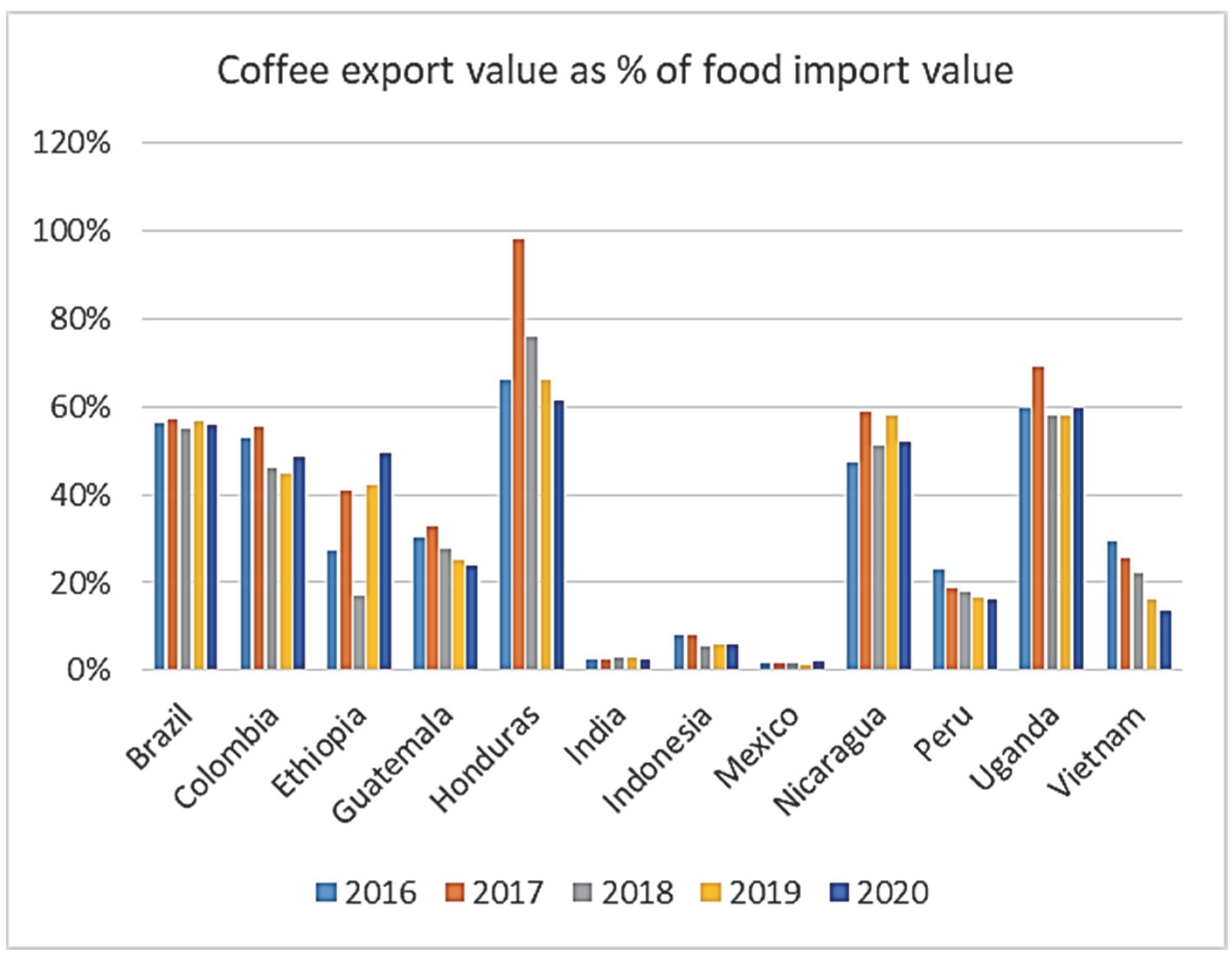
| Countries | Coffee Share in Total Agricultural Export | Coffee Share in Total Merchandise Export | Coffee Export as % of Total Food Import | |||
|---|---|---|---|---|---|---|
| 2018 | 2020 | 2018 | 2020 | 2018 | 2020 | |
| (1) | (2) | (3) | (4) | (5) | (6) | (7) |
| Brazil | 5.3% | 5.8% | 1.8% | 2.4% | 54.9% | 55.7% |
| Colombia | 32.0% | 32.0% | 5.4% | 7.9% | 45.9% | 48.6% |
| Ethiopia | 32.4% | 47.7% | 13.3% | 22.8% | 17.0% | 49.3% |
| Guatemala | 12.9% | 10.7% | 6.3% | 5.7% | 27.9% | 23.7% |
| Honduras | 47.1% | 37.8% | 12.8% | 12.8% | 75.9% | 61.3% |
| India | 1.7% | 1.4% | 0.2% | 0.2% | 2.8% | 2.5% |
| Indonesia | 2.2% | 2.2% | 0.4% | 0.5% | 5.4% | 5.8% |
| Mexico | 1.1% | 1.0% | 0.1% | 0.1% | 1.6% | 1.9% |
| Nicaragua | 20.3% | 19.8% | 8.3% | 8.6% | 51.0% | 51.8% |
| Peru | 10.2% | 8.5% | 1.4% | 1.5% | 18.0% | 16.0% |
| Uganda | 27.0% | 33.8% | 14.1% | 12.4% | 58.0% | 59.7% |
| Vietnam | 15.0% | 10.6% | 1.2% | 0.7% | 22.2% | 13.5% |
| Population Affected by… | Severe Food Insecurity, % | Undernourishment, % | ||
|---|---|---|---|---|
| % | 2016–2018 | 2018–2020 | 2016–2018 | 2018–2020 |
| (1) | (2) | (3) | (4) | (5) |
| Brazil | 1.7 | 3.5 | 2.5 | 2.6 |
| Colombia | na | na | 5.9 | 7.2 |
| Ethiopia | 14.8 | 16.4 | 15.7 | 21.9 |
| Guatemala | 17.1 | 19.2 | 16.3 | 16.3 |
| Honduras | 14.1 | 14.6 | 13.2 | 13.3 |
| India | na | na | 13.2 | 14.6 |
| Indonesia | 0.9 | 0.7 | 5.9 | 6.2 |
| Mexico | 3.3 | 3.9 | 6.1 | 6 |
| Nicaragua | na | na | 17.2 | 17.5 |
| Peru | 16.6 | 19.2 | 7.6 | 8.1 |
| Uganda | 24.5 | 23.3 | no data | no data |
| Vietnam | 0.5 | 0.5 | 7.2 | 6.2 |
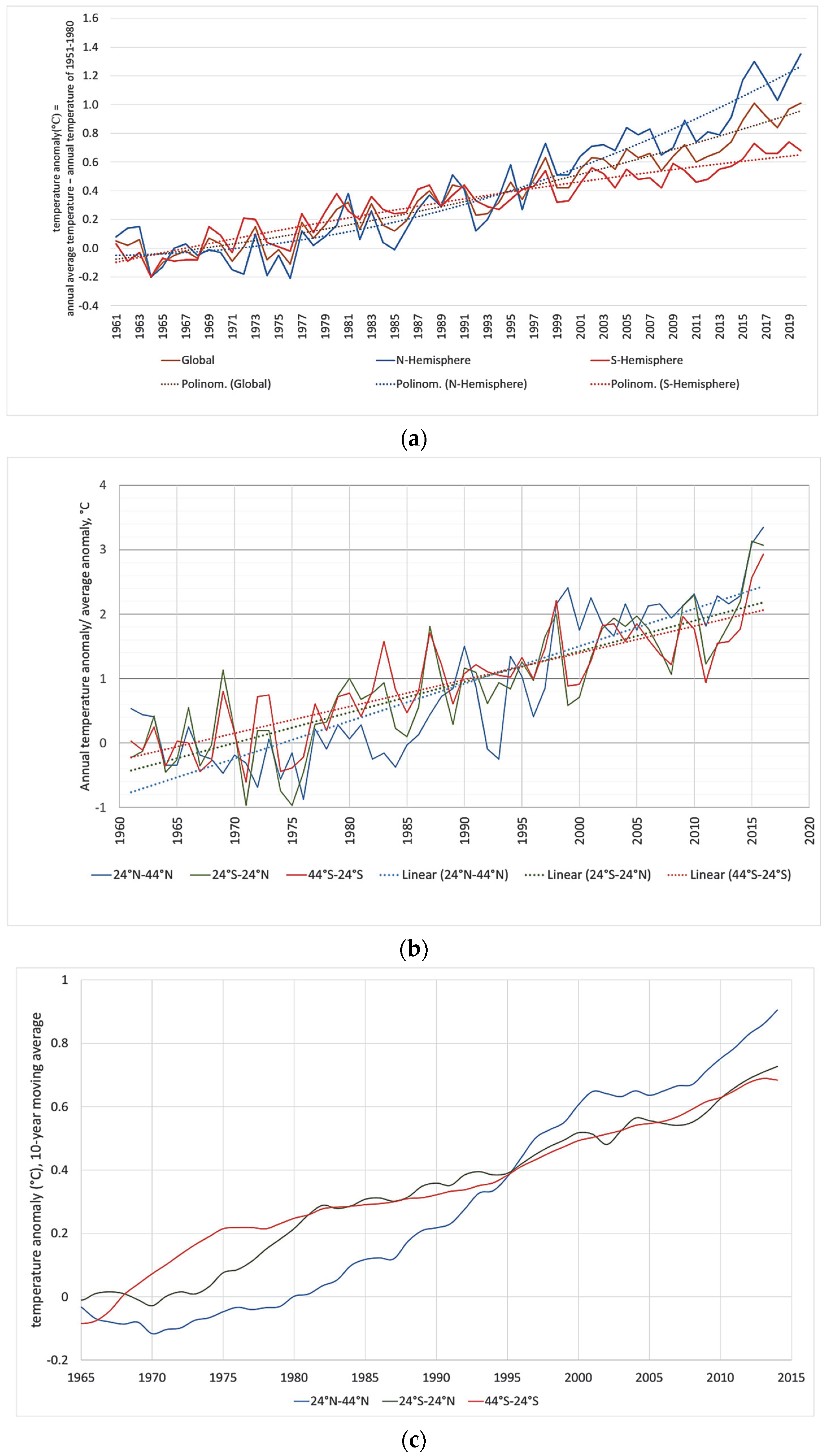
| (1) | (2) | (3) | Max–Min of Trend Values | Absolute Difference in Trend Values | SUM of Absolute Diff’s | 10-Year Moving Averages | |||||
|---|---|---|---|---|---|---|---|---|---|---|---|
| Year | 24 N–44 N Trend | 24 S–24 N Trend | 44 S–24 S Trend | (1)–(2) | (2)–(3) | (1)–(3) | 24 N–44 N | 24 S–24 N | 44 S–24 S | ||
| 1990 | 0.921217 | 0.949045 | 0.982343 | 0.06113 | 0.0278 | 0.03330 | 0.061 | 0.122 | 0.218 | 0.359 | 0.322 |
| 1991 | 0.979352 | 0.996491 | 1.02391 | 0.04456 | 0.0171 | 0.02742 | 0.045 | 0.089 | 0.231 | 0.352 | 0.333 |
| 1992 | 1.037487 | 1.043937 | 1.065477 | 0.02799 | 0.0065 | 0.02154 | 0.028 | 0.056 | 0.277 | 0.385 | 0.338 |
| 1993 | 1.095622 | 1.091383 | 1.107044 | 0.01566 | 0.0042 | 0.01566 | 0.011 | 0.031 | 0.327 | 0.395 | 0.351 |
| 1994 | 1.153757 | 1.138829 | 1.148611 | 0.01493 | 0.0149 | 0.00978 | 0.005 | 0.030 | 0.335 | 0.385 | 0.36 |
| 1995 | 1.211892 | 1.186275 | 1.190178 | 0.02562 | 0.0256 | 0.00390 | 0.022 | 0.051 | 0.379 | 0.39 | 0.384 |
| 1996 | 1.270027 | 1.233721 | 1.231745 | 0.03828 | 0.0363 | 0.00198 | 0.038 | 0.077 | 0.441 | 0.42 | 0.412 |
| 1997 | 1.328162 | 1.281167 | 1.273312 | 0.05485 | 0.0470 | 0.00785 | 0.055 | 0.110 | 0.502 | 0.45 | 0.433 |
| 1998 | 1.386297 | 1.328613 | 1.314879 | 0.07142 | 0.0577 | 0.01373 | 0.071 | 0.143 | 0.528 | 0.475 | 0.455 |
| 1999 | 1.444432 | 1.376059 | 1.356446 | 0.08799 | 0.0684 | 0.01961 | 0.088 | 0.176 | 0.551 | 0.495 | 0.474 |
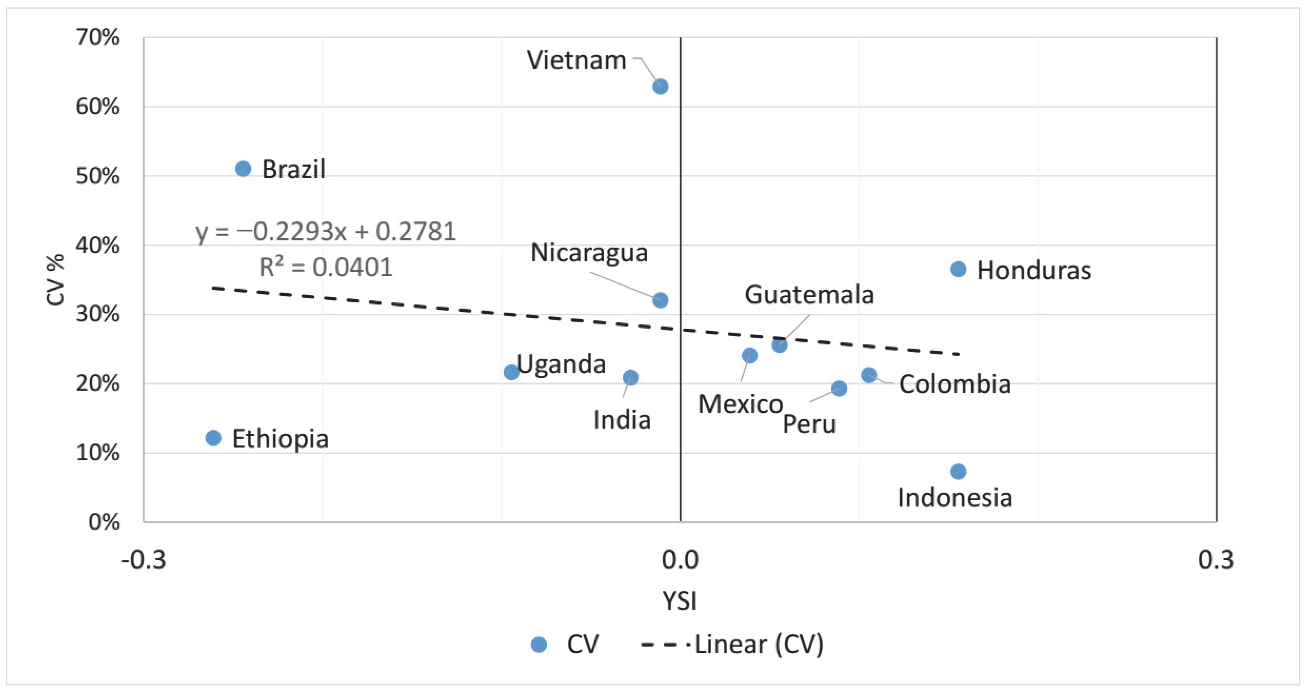
| Countries | Average | CV% | YSI 1961–2020 | Weakly Technologized | Shapiro–Wilk Test |
|---|---|---|---|---|---|
| (1) | (2) | (3) | (4) | (5) | p > 0.05 (0.01) |
| Brazil | 804.0 | 51.1% | −0.245 | x | 0.1528 * |
| Vietnam | 1334.4 | 62.9% | −0.011 | x | 0.3406 * |
| Colombia | 766.1 | 21.2% | 0.105 | 0.1861 * | |
| Indonesia | 551.2 | 7.3% | 0.155 | 0.0495 ** | |
| Ethiopia | 703.0 | 12.2% | −0.261 | x | 0.0439 ** |
| Peru | 632.3 | 19.3% | 0.089 | 0.6117 * | |
| Honduras | 699.5 | 36.6% | 0.155 | 0.8438 * | |
| India | 720.1 | 20.9% | −0.028 | x | 0.2597 * |
| Uganda | 638.7 | 21.6% | −0.095 | x | 0.3678 * |
| Guatemala | 773.6 | 25.6% | 0.055 | 0.8130 * | |
| Mexico | 456.6 | 24.1% | 0.039 | 0.8873 * | |
| Nicaragua | 624.1 | 32.1% | −0.011 | x | 0.3720 * |
| Countries | 1961–1994 | 1995–2020 | YSI(2)–YSI(1) | ||||
|---|---|---|---|---|---|---|---|
| AVG Yield | CV% | YSI(1) | AVG Yield | CV% | YSI(2) | ||
| (1) | (2) | (3) | (4) | (5) | (6) | (7) | (8) |
| Brazil | 533.4 | 24.5% | −0.1929 | 1157.9 | 32.9% | 0.0493 | 0.2422 |
| Vietnam | 704.0 | 66.6% | −0.2223 | 2158.8 | 16.4% | −0.0277 | 0.1946 |
| Colombia | 679.7 | 19.4% | 0.0130 | 879.0 | 14.5% | −0.0661 | −0.0791 |
| Indonesia | 566.1 | 4.8% | 0.0424 | 531.6 | 8.8% | 0.0877 | 0.0453 |
| Ethiopia | 732.7 | 2.4% | n.a. | 700.7 | 12.6% | −0.0277 | −0.0113 |
| Peru | 544.6 | 7.7% | 0.0424 | 747.0 | 12.5% | 0.0108 | −0.0316 |
| Honduras | 519.8 | 29.3% | 0.0424 | 934.6 | 15.9% | 0.0877 | 0.0453 |
| India | 648.3 | 23.6% | −0.0752 | 814.1 | 9.7% | 0.1262 | 0.2014 |
| Uganda | 629.1 | 22.1% | −0.1340 | 651.3 | 21.4% | −0.1046 | 0.0294 |
| Guatemala | 647.3 | 21.9% | 0.0424 | 938.7 | 13.5% | 0.0108 | −0.0316 |
| Mexico | 527.4 | 13.1% | 0.0130 | 363.9 | 22.1% | 0.1262 | 0.1132 |
| Nicaragua | 506.8 | 26.7% | −0.0752 | 777.5 | 21.2% | −0.1430 | −0.0678 |
Publisher’s Note: MDPI stays neutral with regard to jurisdictional claims in published maps and institutional affiliations. |
© 2022 by the authors. Licensee MDPI, Basel, Switzerland. This article is an open access article distributed under the terms and conditions of the Creative Commons Attribution (CC BY) license (https://creativecommons.org/licenses/by/4.0/).
Share and Cite
Bacsi, Z.; Fekete-Farkas, M.; Ma’ruf, M.I. Coffee Yield Stability as a Factor of Food Security. Foods 2022, 11, 3036. https://doi.org/10.3390/foods11193036
Bacsi Z, Fekete-Farkas M, Ma’ruf MI. Coffee Yield Stability as a Factor of Food Security. Foods. 2022; 11(19):3036. https://doi.org/10.3390/foods11193036
Chicago/Turabian StyleBacsi, Zsuzsanna, Mária Fekete-Farkas, and Muhammad Imam Ma’ruf. 2022. "Coffee Yield Stability as a Factor of Food Security" Foods 11, no. 19: 3036. https://doi.org/10.3390/foods11193036
APA StyleBacsi, Z., Fekete-Farkas, M., & Ma’ruf, M. I. (2022). Coffee Yield Stability as a Factor of Food Security. Foods, 11(19), 3036. https://doi.org/10.3390/foods11193036