Phase Relations in the Pseudo-Binary BiFeO₃–EuFeO₃ System in the Subsolidus Region Derived from X-Ray Diffraction Data—A Machine Learning Approach

Abstract

BiFeO₃ and EuFeO₃ are some of the most studied ferrites and part of the larger category of multiferroic and magnetic compounds. The instabilities reported for BiFeO₃ that hinder its use in practical applications can be overcome by substitution with rare-earth ions, such as Eu³⁺, on the Bi³⁺ site. This paper reports on the phase relations in the BiFeO₃-EuFeO₃ pseudo-binary system, which were not established previously. Solid-state reactions were employed to prepare different compositions according to the nominal formula Bi_1−xEu_xFeO₃ (where x = 0, 0.05, 0.10, 0.15, 0.2, 0.3, 0.4, 0.5, 0.6, 0.7, 0.8, 0.9, and 1). Phase equilibria were studied at different temperatures between 800 and 1200 °C from X-ray diffraction (XRD) data. The analysis of the XRD patterns by machine learning approaches revealed eight defined clusters and four unclustered points. The validation test showed that most of the points could belong to several clusters and thus, traditional identification was employed. Phase identification and quantification by traditional approaches revealed six crystallization zones on the diagram. Although the machine learning approach offers speed in the process of classification of XRD patterns, validation by the traditional method was necessary for the construction of the phase diagram with high accuracy.

1. Introduction

Multiferroic and magnetic compounds have garnered significant attention in materials science and engineering for their unique electrical, magnetic, and structural properties [1,2,3,4]. Intelligent materials include those with couplings between order parameters such as the magnetoelectric effect evidenced in some multiferroics [5,6,7].

Foundational work by G. A. Smolenskii and V. A. Bukov in 1964 [8] evidenced the coexistence of magnetic and electric ordering in crystals. In their work, they investigated the YMnO₃, and YbMnO₃, which showed both ferroelectricity and antiferromagnetism and developed a thermodynamic theory describing materials which are simultaneously ferroelectric and ferromagnetic. These observations fuelled research activities in solid-state physics and materials science. In 1969, K. Aizu described materials with two orientation states as “ferroic” and classified them into ferroelectrics, ferromagnetics, and ferroelastics [9]. In addition, Aizu’s work emphasized the theoretically possible symmetries and point groups of ferroelectric, ferroelastic and simultaneously ferroelectric and ferroelastic crystals. In 1994, H. Schmid established the term “multiferroic” for a “material exhibiting two or more ferroic orders simultaneously” [10]. There is, however, a distinction between this type of materials and materials where the ferroic order parameters are coupled. The coupling between the order parameters (ferromagnetism, ferroelectricity, and ferroelasticity) results in various phenomena, such as magnetoelectric, piezoelectric, and magnetoelastic coupling. During the following years, the efforts in solid-state physics and materials science enabled the identification of mechanisms that drive multiferroicity (lone-pair mechanism, geometric ferroelectricity, ferroelectricity due to charge ordering, magnetically induced ferroelectricity) [11].

Among magnetoelectric multiferroics, one of the most studied compounds is BiFeO₃. The interest in this compound is owed to its room-temperature magnetoelectric coupling, combining ferroelectric and antiferromagnetic orders [12,13,14,15,16]. This rare property among single-phase materials has pointed to extensive research efforts into its use in spintronic devices [17,18,19], data storage systems [20,21,22], and electro-optical applications [23,24,25,26,27]. The interplay between its electric polarization and magnetic ordering enables potential applications where control over both degrees of freedom is crucial.

BiFeO₃ is a binary oxide compound placed in the Bi₂O₃-Fe₂O₃ phase diagram. The phase diagram of this oxide system is presented in Figure 1, showing three different compounds: Bi₂₅FeO₃₉, BiFeO₃, and Bi₂Fe₄O₉.

In the Bi₂O₃-rich part, Bi₂₅FeO₃₉ is illustrated as a liquid incongruent binary compound, which decomposes into Bi₂O₃ and liquid at a temperature of 795 °C. In the Fe₂O₃-rich part, Bi₂Fe₄O₉ is a liquid incongruent binary compound that decomposes into Fe₂O₃ and liquid at 960 °C. The multiferroic compound, BiFeO₃, an equimolar mixture of Bi₂O₃ and Fe₂O₃, is also a liquid incongruent binary compound. This compound decomposes into Bi₂Fe₄O₉ and liquid at a temperature of 930 °C. Between room temperature and the peritectic decomposition temperature, BiFeO₃ goes through a polymorphic transition from α to β phase at 825 °C.

Furthermore, instability of the BiFeO₃ compound has been evidenced since the 1970s, when Skinner et al. [29] encountered difficulties in determining the Curie temperature due to a slow decomposition starting at 700 °C, even below the sublimation temperature of Bi₂O₃. The experimental and theoretical studies of Selbach et al. [30] showed that in the 447–767 °C temperature range, BiFeO₃ decomposes into Bi₂Fe₄O₉ (mullite-type phase) and Bi₂₅FeO₃₉ (sillenite-type phase). At the same time, at temperatures between 775 and 850 °C, BiFeO₃ is also the product of the reaction of the two compounds, according to the chemical reaction equation:

$${\displaystyle \raisebox{1ex}{$1$}\!\left/ \!\raisebox{-1ex}{$49$}\right.}{\mathrm{Bi}}_{25}\mathrm{Fe}{\mathrm{O}}_{39}+{\displaystyle \raisebox{1ex}{$12$}\!\left/ \!\raisebox{-1ex}{$49$}\right.}{\mathrm{Bi}}_2{\mathrm{Fe}}_4{\mathrm{O}}_9\rightleftharpoons \mathrm{BiFe}{\mathrm{O}}_3$$

The instability of BiFeO₃ hinders its use in practical applications. Thus, several attempts were made to offer alternative routes for the synthesis of BiFeO₃ in order to avoid its decomposition. The strategies adopted by the scientific community are the use of wet synthetic methods and doping/substitution on the Bi³⁺ or Fe³⁺ sites [31].

Attempts to stabilize and enhance the magnetic behaviour of BiFeO₃ by substitution were predominantly aimed at replacing Bi³⁺ with rare-earth ions (RE), taking into account the similarity between the ionic radius and the superexchange interactions between the localized RE4f and Fe3d electrons [32]. Thus, the effect of several rare-earth dopants/solutes such as Ho, Sm, La, Dy, Gd, Nd, or Eu were reported concerning BiFeO₃ phase stabilization and magnetic or electrical behaviour [33,34,35,36,37,38,39,40,41,42,43,44,45]. Rare earth ferrites exhibit a distorted non-polar perovskite structure of orthorhombic symmetry. Thus, compositions in Bi_1−xRE_xFeO₃ systems are expected to change symmetry from polar R3c (symmetry of pristine BiFeO₃) to a non-polar space group by an increase in the amount of rare earth oxide.

The structural transition between rhombohedral and orthorhombic phases for Bi_1−xLa_xFeO₃ has been investigated by Karpinsky et al. [46]. They proposed two models: the first one assumed that there is a coexistence of different nanoscale structural phases which can be interpreted as a phase with lower, monoclinic symmetry; the second one assumes that the phases are defined by a spatially modulated structure by the ground state energy. The X-ray and neutron diffraction experiments on the Bi_1−xLa_xFeO₃ system showed that materials with x ≤ 0.15 possess a rhombohedral symmetry; the material with x = 0.20 can be described by the orthorhombic Pbam symmetry; and materials with x > 0.50 exhibit Pnma symmetry [47]. In the intermediate region 0.16 ≤ x ≤ 0.20 a mixture of rhombohedral R3c and Pbam symmetries coexist, while in the region 0.45 ≤ x ≤ 0.50 a mixture of orthorhombic Pbam and Pnma can be identified [48]. Troyanchuk et al. identified another symmetry in the region 0.4 < x < 0.5 with orthorhombic Imma space group [49].

In the Bi_1xGd_xFeO₃ system, there are several reports on the phase stability and structures. Thus, for x ≤ 0.10, rhombohedral R3c symmetry was reported as stable [50]. Upon increasing the gadolinium content, the structural phase transitions R3c → Pn2₁a (for the region 0.10 < x < 0.20) and Pn2₁a → Pnma (for the compositional range 0.10 < x < 0.30) take place as evidenced by Khomchenko et al. [51]. However, the experimental studies are controversial and identified a mixture of R3c, Pbam and Pn2₁a phases for a composition with x = 0.15.

In the Bi_1−xDy_xFeO₃ system, Pattanayak et al. and Xu et al. [52,53] reported compositions exhibiting R3c symmetry for the compositional range with x ≤ 0.20. A. C. Donna [54] suggested a monoclinic Cc symmetry for 0.06 ≤ x ≤ 0.20.

Most of the work available in the scientific literature regarding the Bi_1−xEu_xFeO₃ system involves the effect of Eu substitutions on the magnetic or electrical properties and pays limited attention to the phase relationships between BiFeO₃ and EuFeO₃. In addition, no information is available about the phase diagram of the ternary Bi₂O₃–Eu₂O₃–Fe₂O₃ system.

EuFeO₃ is a member of the rare-earth orthoferrites, important due to its magnetic and electronic properties [55,56]. EuFeO₃ is a binary oxide placed in the Eu₂O₃–Fe₂O₃ phase diagram, illustrated in Figure 2. The phase diagram shows the existence of two solid compounds: EuFeO₃ and Eu₃Fe₅O₁₂. The available data in the subsolidus region show the following primary crystallization fields:

(i)

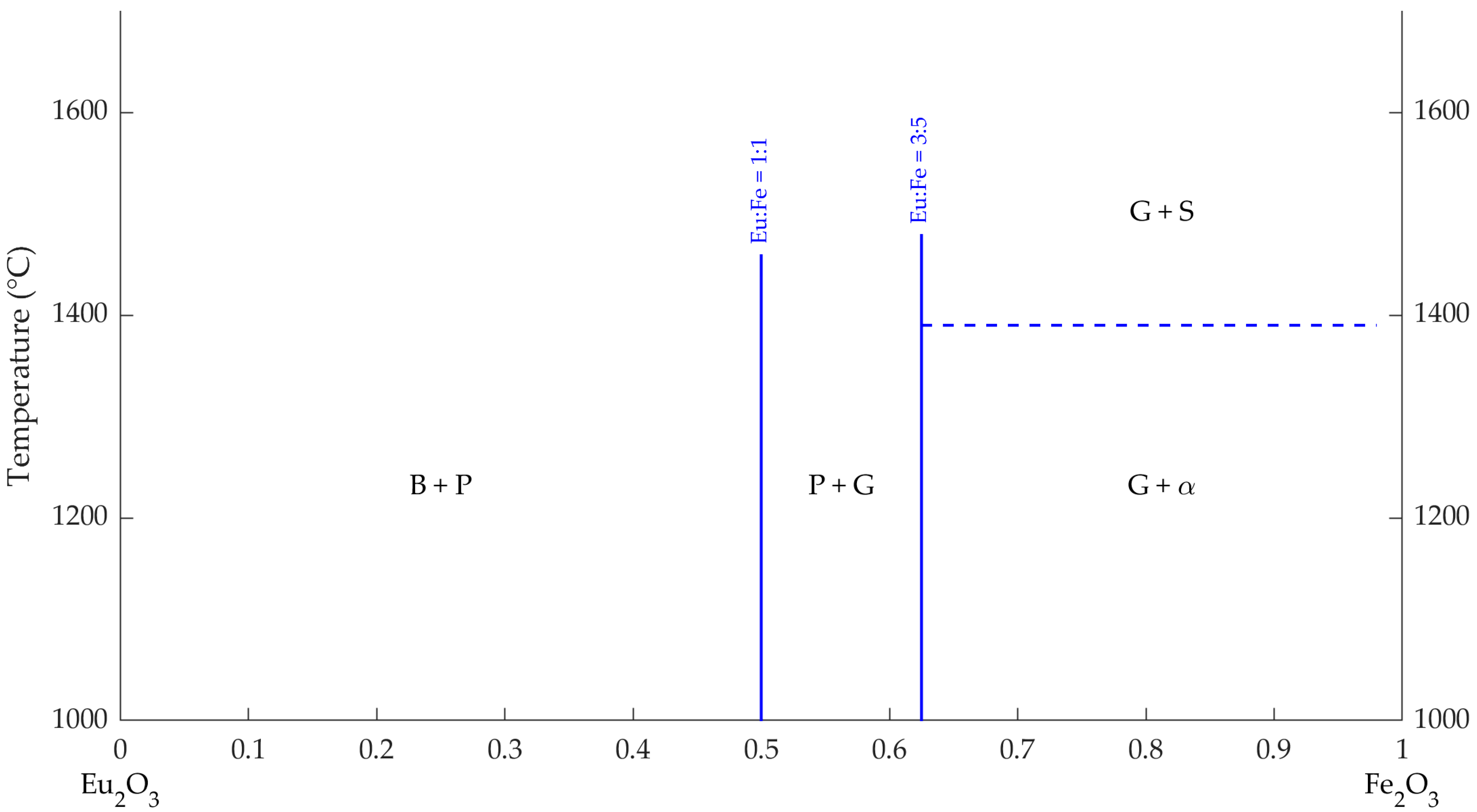
In the (left-hand side) composition region having 50 mol% Fe₂O₃ or less, and temperatures between 1000 and 1450 °C, crystallization of a mixture of B-type Eu₂O₃ and perovskite-type EuFeO₃ occurs;

(ii)

The region delimited by 50 and 62.5 mol% Fe₂O₃ and temperatures between 1000 and 1450 °C is characterized by the crystallization of a mixture of perovskite-type EuFeO₃ and garnet type Eu₃Fe₅O₁₂;

(iii)

In the region delimited by 62.5 and 100 mol% Fe₂O₃, at temperatures between 1000 and 1400 °C, the crystallization of garnet type Eu₃Fe₅O₁₂ and corundum-type phase (α) can be observed; at higher temperatures for the same composition range, the corundum-type phase suffers a polymorphic transition to the spinel structure.

The reports on the solid solutions between BiFeO₃ and EuFeO₃ mention only part of the composition range in the pseudo-binary system, mainly in the BiFeO₃-rich region [58,59,60,61]. Thus, materials with x ≤ 0.10 were found with R3c symmetry [38,62,63], and materials with x ≥ 0.20 were reported with Pnma symmetry [64]. The available data are not consistent regarding the synthesis of the compositions, with several synthesis methods being employed by different research teams: solid-state, sol-gel, or combustion synthesis. Thus, for a better understanding of the phase relations in this system, a systematic study should be employed.

In this paper, we report the phase relations over the entire compositional system BiFeO₃–EuFeO₃ derived from X-ray diffraction data analysis of solid-state prepared specimens. We also considered this lesser-known oxide system for the application of machine learning techniques (cluster analysis) to accelerate the process of classification and grouping of X-ray diffraction data [65]. Machine learning, together with phase identification and quantification approaches to construct a phase diagram from X-ray diffraction data, is discussed.

2. Materials and Methods

2.1. Materials Processing

Different compositions in the BiFeO₃–EuFeO₃ oxide pseudo-binary system were prepared according to the nominal formula Bi_1−xEu_xFeO₃ (where x = 0; 0.05; 0.10; 0.15; 0.20; 0.30; 0.40; 0.50; 0.60; 0.70; 0.80; 0.90; 1) by solid-state reactions route.

The raw materials (Bi₂O₃, 99.9%, Fe₂O₃, ≥99.995%, Eu₂O₃, 99.9%, and 2-Propanol, 99.5% anhydrous) were purchased from Sigma-Aldrich (St. Louis, MO, USA) and used without further purification.

Mixtures of oxides were prepared by weighting and mixing the components in 2-Propanol medium in an agate mortar until volatilization of the liquid (≈1 h). The mass composition of the mixtures is given in

Table 1. Oxide mixture compositions. All three raw materials were purchased from Sigma-Aldrich (St. Louis, MO, USA).

Composition	Bi2O3 Content (g)	Eu2O3 Content (g)	Fe2O3 Content (g)
BiFeO3	11.6490	0	3.9922
Bi0.95Eu0.05FeO3	11.0665	0.4399	3.9922
Bi0.90Eu0.10FeO3	10.4841	0.8798	3.9922
Bi0.85Eu0.15FeO3	9.9016	1.3197	3.9922
Bi0.80Eu0.20FeO3	9.3192	1.7596	3.9922
Bi0.70Eu0.30FeO3	8.1543	2.6394	3.9922
Bi0.60Eu0.40FeO3	6.9894	3.5193	3.9922
Bi0.50Eu0.50FeO3	5.8245	4.3991	3.9922
Bi0.40Eu0.60FeO3	4.6596	5.2789	3.9922
Bi0.30Eu0.70FeO3	3.4947	6.1587	3.9922
Bi0.20Eu0.80FeO3	2.3298	7.0385	3.9922
Bi0.10Eu0.90FeO3	1.1649	7.9183	3.9922
EuFeO3	0	8.7982	3.9922

.

The mixtures were uniaxially pressed under a pressure P = 180 MPa and pre-sintered at a temperature of 800 °C for 1 h with a heating rate of 5 °C/min. The pre-sintered ceramic bodies were ground in an agate mortar and reshaped by uniaxial pressing. The final ceramic bodies were obtained after a sintering step at different temperatures (850, 875, 900, 925, 950, 975, 1000, 1100, and 1200 °C) depending on the composition for 1 h with a heating rate of 5 °C/min. The maximum sintering temperature was kept below the initial melting point of the subjected composition.

2.2. X-Ray Diffraction Characterization

Phase composition was investigated for polished sintered samples using a PANalytical Empyrean X-ray diffractometer (Cedar Park, TX, USA) operated in reflection theta–theta geometry at room temperature. The instrument was equipped with a CuKα (λ = 1.5418 Å) sealed X-ray tube with a fixed 1/4° divergence slit and fixed 1/2° anti-scatter slit on the incident beam side, and, respectively, on the diffracted beam side, a 1/2° anti-scatter slit, and a Ni-filter mounted on the PIXCel3D detector. The detector was used in scanning line mode (1D), which means the detector was moved over the 2θ range of interest at each step along the scan; the intensity at a particular 2θ position (data point) was measured and then summed, until the data point was no longer in range. The total opening of the detector was approximately 3.3°. The analyses were conducted in the 20–80° 2θ range, with a step size of 0.026° and a counting time per step of 255 s, with a full revolution at each step. The recorded patterns showed a higher than 10:1 peak-to-background ratio and over seven points over the full width at half maximum, depicting a good quality of the data. The recorded patterns were subjected to phase identification and quantification and cluster analysis in HighScore Plus 3.0.e software using profile and peaks comparison and the reference scan database from the International Centre for Diffraction Data (ICDD PDF5+).

In the traditional approach to phase diagram determination, the patterns were treated before analysis using a polynomial background determination, Rachinger Kα₂ stripping method [66] and peak search by using the minimum second derivative criterion. The reduced patterns were subjected to a search and match procedure using the ICDD PDF-5+ database. The qualitatively identified patterns were converted to phases and the quantification was performed by using a Rietveld refinement algorithm with a polynomial function for background approximation, a pseudo-Voigt function for peak profile, and a Caglioti function for peak width.

In the machine learning approach, cluster analysis was performed on the same data using HighScore Plus software 3.0.e. First, the raw datasets were reduced to probability curves. Then, the data for all pairs of XRD patterns were compared to calculate the similarity coefficients encoded in the correlation matrix. The correlation matrix was converted into a Euclidian distance matrix and the linkage method was used to perform the agglomerative hierarchical clustering. The optimum number of clusters was determined using the Kelley, Gardner and Sutcliffe (KGS) method [67]. Cluster validation was performed by the Silhouette index method and the membership of a dataset to more than one cluster was assessed using Fuzzy clustering.

3. Results and Discussion

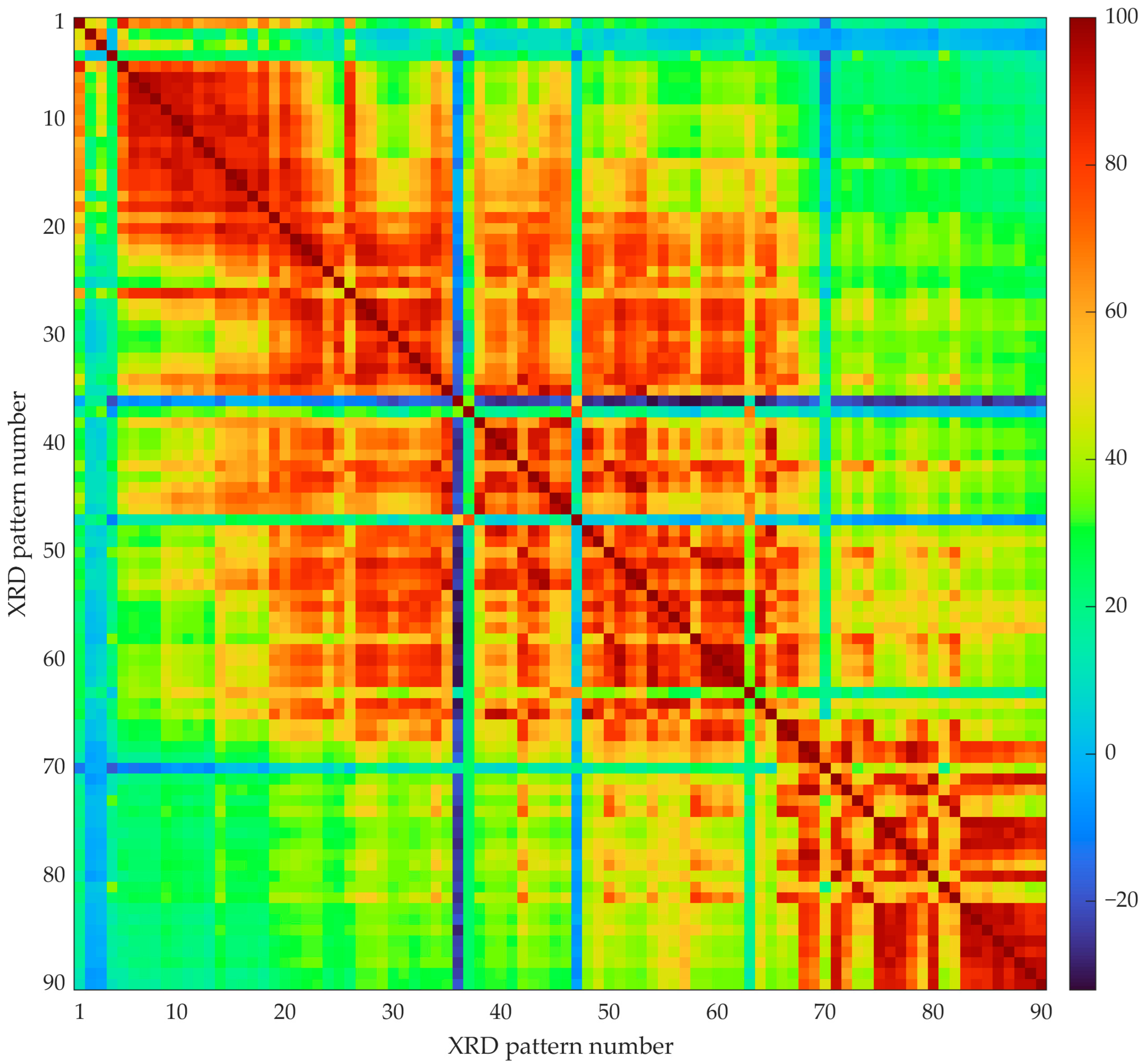
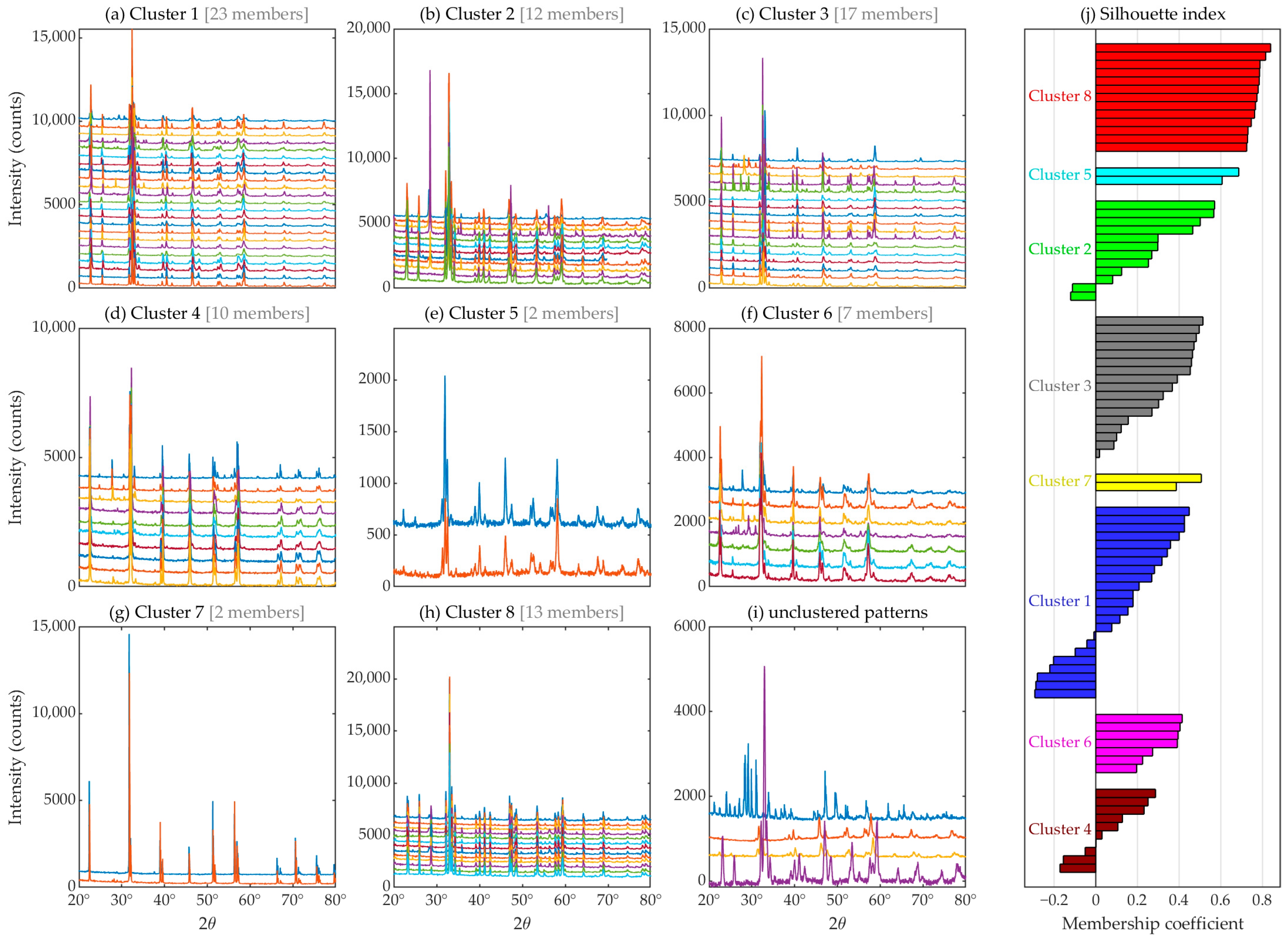
3.1. Automated Approach: Unsupervised Machine Learning (Clustering)

Unsupervised machine learning was employed to classify the X-ray diffraction patterns using peak position and peak intensity as features, which were automatically determined by the clustering software, HighScore Plus 3.0.e. In the first step, all measured raw datasets were reduced to probability curves $u_i\left(x\right)$, which describes the probability for every data point at position $x$ to hold an intensity significantly above the background level. Each possible pair of probability curves is then compared. The quality of the match between the two datasets was based on scores assigned to matching 2θ positions of the peaks. The peak position score consists of the sum of the probability curves divided by the number of matching lines. The similarity between the pairs of the 90 recorded diffraction patterns resulted in a $90\times 90$ correlation matrix $p$ (Figure 3) using the features inferred previously. While most of the diffraction patterns are at least partially correlated with other XRD patterns, several of them present low correlation or even inverse correlation with most of the data points; the latter points are expected to cluster together or to be left non-clustered.

The resulting correlation matrix was then fed into the agglomerative hierarchical clustering algorithm. Thus, the correlation matrix $p$ was converted into a Euclidean distance matrix $d$ of the same dimension ($d=1-p$). At the beginning of the clustering algorithm, each diffraction pattern was allocated to a distinct cluster. At all subsequent steps of the analysis, two clusters with the highest degree of similarity were merged into a single cluster. The distance measure between clusters was calculated using squared Euclidian distance (Equation (1)).

$$D_{i,j}=\sum _{k=1}^N{\left(C_{k,i}-C_{k,j}\right)}^2$$

(1)

where $D_{i,j}$ was the dissimilarity between object $i$ and $j$, and $C_{k,i}$ is the value that the object $i$ took on the character $k$.

The linkage method used for the agglomerative hierarchical analysis, which describes how distances between clusters are used to join two clusters was the average linkage method. Thus, the average similarity of observations between the two groups was used as the measure between the two groups. Each observation had the same weight when combining groups, meaning that groups with more observations had more influence on the determination of the combined group.

The optimal number of clusters was determined using the method introduced by Kelley, Gardner and Sutcliffe (KGS method), which looks for the state $icut$, where the clusters are as highly populated as possible, whilst simultaneously maintaining the smallest spread within the clusters [67]. The distance matrix $d$ is used as input for the KGS test. At each step of clustering, the “spread” of each cluster was calculated. The spread of a cluster $m$ containing $n$ members was calculated by Equation (2):

$${spread}_m={\displaystyle \frac{\left({\sum }_{k=1}^N{\sum }_{i=1,j>k}^{N}dist(i,k)\right)}{N\cdot (N-1)/2}}$$

(2)

where $k$ and $i$ are members of the cluster $m$.

The average spread was calculated by Equation (3):

$$Av{Sp}_i={\displaystyle \frac{{\sum }_{m=1}^{{cnum}_i}{spread}_m}{{cnum}_i}}$$

(3)

where ${cnum}_i$ was the number of clusters at the stage $i$ of the clustering (excluding outliers).

Once clustering was complete, the set of $Av{Sp}_i$ values were normalized to lie within the range of 1 to $N-1$, where $N$ was the total number of datasets. Normalization was used to achieve equal weight in the penalty function to the number of clusters and the average spread (Equation (4)).

$${AvSp\left(norm\right)}_i=\left({\displaystyle \frac{N-2}{Max\left(AvSp\right)-Min\left(AvSp\right)}}\right)\cdot \left({AvSp}_i-Min\left(AvSp\right)\right)+1$$

(4)

where $Max\left(AvSp\right)$ and $Min\left(AvSp\right)$ are the maximum and minimum values, respectively, of $AvSp$ in the set $\left\{{AvSp}_1,{AvSp}_2\dots {AvSp}_{N-1}\right\}$.

For each clustering stage $i$, a penalty value, $P_i$, was calculated as shown in Equation (5):

$$P_i={AvSp\left(norm\right)}_i+{nclus}_i$$

(5)

where ${nclus}_i$ was the total number of clusters at step $i$ of the clustering (including outliers).

A representation of the penalty value versus the number of clusters in the dataset is illustrated in Figure 4.

The minimum penalty value (Equation (6)) in the set $\{P1,P2,\dots ,P_{N-1}\}$ was chosen as the cut-off level for the dendrogram (Figure 5).

$$P_{icut}=Min\left(P\right)$$

(6)

The KGS method outputs two pieces of information: the optimal number of clusters according to its penalty function, and a cutoff (maximum) value for the distance between adjacent clusters. The total number of clusters obtained from the analysis is 12, with 8 proper clusters (i.e., containing at least two members), and 4 non-clustered X-ray diffraction patterns. The agglomerative hierarchical clustering results are visualized as a dendrogram in Figure 5, including the cutoff point that determined the number of clusters.

The silhouette index [68] was used to evaluate the quality of the clustering. Silhouettes show the coefficient of membership of each cluster member in a histogram. The distance matrix $d$ was converted into the dissimilarity matrix $\delta$ (Equation (7)).

$$\delta =d_{ij}/d_{ij}^{max}$$

(7)

If the pattern $i$ belongs to cluster $C_r$, which contains $n_r$ patterns, an average dissimilarity of the pattern $i$ with respect to all other patterns in the cluster $C_r$ was defined by using Equation (8):

$$a_i=\sum _{jϵC_{r}j\ne i}{\delta }_{ij}/\left(n_r-1\right)$$

(8)

The minimum dissimilarity of cluster $C_r$ was defined by Equation (9):

$$b_i={min}_{s\ne r}\left(\sum _{jϵC_{r}j\ne i}{\delta }_{ij}/n_s\right)$$

(9)

The silhouette for pattern $i$ was then defined using Equation (10):

$$S\left(i\right)={\displaystyle \frac{\left(b\left(i\right)-a\left(i\right)\right)}{max\left\{a\left(i\right),b\left(i\right)\right\}}}$$

(10)

Silhouette values range between −1 and +1; values close to +1 indicate the correct assignment of points to clusters, while negative values indicate that those points are more likely to belong to other clusters than the one that they were assigned to. The obtained clusters of XRD patterns and associated silhouettes corresponding to the coefficient of membership of each cluster are illustrated in Figure 6. Interestingly, the patterns with low values in the correlation matrix (visualized in Figure 3 as a heatmap) were either grouped together in clusters with low member counts or were not clustered by the analysis. Based on the silhouette plots (Figure 6j), several points from cluster 1 seem to be misallocated, as well as a few points from clusters 2 and 4.

Finally, the phase diagram was constructed by plotting each XRD pattern at the coordinates, given by composition and temperature (Figure 7); the colour for each data point was chosen according to the index assigned by the agglomerative clustering algorithm. Disregarding the non-clustered points, the assigned cluster indices seem to divide the composition–temperature space into three regions: the left side of the diagram is defined by clusters 4, 6 and 7, the right side by clusters 2 and 8, leaving a mixture of clusters 1, 3 and 5 in the central region of the phase diagram. Unfortunately, the identified regions are not contiguous (particularly, the middle and the right side of the diagram, where several points assigned to clusters 1, 2 and 3 form islands within points assigned to other clusters). Additionally, no information about the phase composition or number of phases in each region is evident from these results, since the clustering algorithm merely identified patterns within the data with no reliable physical interpretation.

The silhouette for cluster 2 shows a couple of points with negative membership coefficients (Figure 6j). At the same time, the phase diagram shows an “intrusion” of cluster 2 into a region predominantly described by cluster 8 (Figure 7, x = 0.8–0.9 and temperature of 950–975 °C). Furthermore, the cluster hierarchy shows that the next step for clusters 2 and 8 is to be merged into a larger cluster (Figure 5), although the linkage distance is rather large (about twice the cutoff value). All these observations suggest that the regions assigned to clusters 2 and 8 may have similar phase composition.

The silhouette plot for cluster 1 shows that about one-third of the XRD patterns in the cluster may be classified incorrectly (Figure 6j), given their negative membership coefficient. Furthermore, XRD patterns that belong to cluster 1 are spread out over the phase diagram, with the larger cluster-1 region being interrupted by patterns belonging to clusters 3 and 5 (at and near x = 0.3) and one isolated pattern at x = 0.7 and T = 1000 °C also belonging to cluster 1 (Figure 7).

Although cluster 4 also contains points with negative membership coefficients, it is unclear which other cluster they might belong to, based solely on the cluster arrangement in the phase diagram shown in Figure 7.

To further test the validity of the membership of each XRD pattern to join more than one cluster, the Fuzzy Clustering validation technique was employed. The results are presented in Table S1. In this table, for each data point, the probability of joining every cluster is assigned. The datapoints which showed a probability above 0.85 indicate that a certain member belongs to a specific cluster only. Thus, in cluster 8, there are ten compositions which can be assigned only to this specific cluster (x = 0.9 for processing temperatures of 875, 900 and 1000 °C and x = 1 for processing temperatures of 900, 950, 975, 1000, 1100, and 1200 °C). Most of the data points show probability values between 0.15 and 0.85 for three or four clusters, which means that they can join several clusters or/and that there is a presence of mixtures in the dataset. To better understand the phase relations in the BiFeO₃–EuFeO₃ binary system, the traditional processing of X-ray diffraction data was employed.

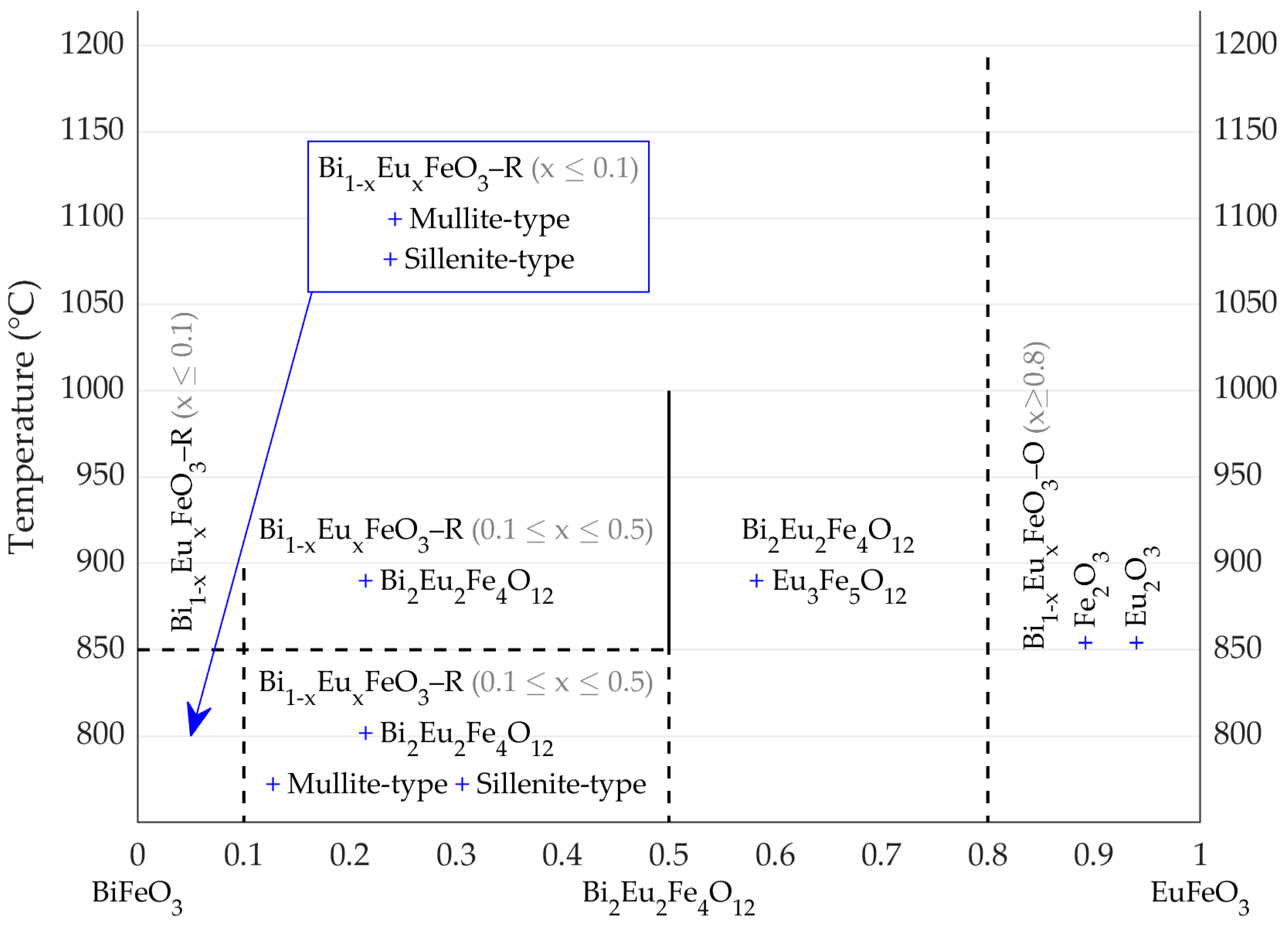
3.2. Traditional Approach

The results of the traditional processing of X-ray diffraction data by phase identification followed by Rietveld refinement are summarized in Table S2. The data include the identifier of the composition, x, which is used in designated specimens of different nominal compositions Bi_1−xEu_xFeO₃, the temperature of processing, and the content of the different identified phases: (Bi,Eu)FeO₃ with rhombohedral symmetry and space group R3c (ICDD PDF 5+ #01-084-7216), Sillenite-type phase (ICDD PDF 5+ #04-008-8064), Mullite-type phase (ICDD PDF 5+ #00-025-0090), Bi₂O₃ (ICDD PDF 5+ #04-023-7254), Bi₂Eu₂Fe₄O₁₂ with orthorhombic symmetry and space group Pnma (ICDD PDF 5+ #04-026-9572), (Bi,Eu)FeO₃ with orthorhombic symmetry and space group Pbnm (ICDD PDF 5+ #00-047-0066), Eu₃Fe₅O₁₂ (ICDD PDF 5+ #04-002-8015), Eu₂O₃ (ICDD PDF 5+ #01-083-7117), and Fe₂O₃ (ICDD PDF 5+ #04-008-8479). Although the clustering results presented in Figure 7 do not supply any information about the phase composition of each sample, they helped guide the traditional approach by informing the order in which to process the diffraction patterns (XRD clusters were processed together). Moreover, the Fuzzy Clustering validation results were taken into account when performing the analysis, by considering the membership to one of the clusters where a datapoint had shown a probability between 0.15 and 0.85.

The obtained results were then grouped by the phase composition and a phase diagram was proposed (Figure 8). There are six composition zones defined as follows:

(1)

Bi_1−xEu_xFeO₃–R (x < 0.1) + Mullite-type + Sillenite-type;

(2)

Bi_1−xEu_xFeO₃–R (x < 0.1);

(3)

Bi_1−xEu_xFeO₃–R (0.1 < x < 0.5) + Bi₂Eu₂Fe₄O₁₂ + Mullite-type + Sillenite-type;

(4)

Bi_1−xEu_xFeO₃–R (0.1 < x < 0.5) + Bi₂Eu₂Fe₄O₁₂;

(5)

Bi₂Eu₂Fe₄O₁₂ + Eu₃Fe₅O₁₂;

(6)

Bi_1−xEu_xFeO₃–O (x ≥ 0.8) + Fe₂O₃ + Eu₂O₃.

The proposed phase diagram indicates the existence of three solid solutions: at x = 0.1 (a solid solution of rhombohedral symmetry), x = 0.5 (Bi₂Eu₂Fe₄O₁₂ Berry phase [69], a complex perovskite which was theoretically predicted and is stable at temperatures ranging between 850 °C and 1000 °C, indicated using a solid vertical line in Figure 8), and x = 0.8 (a solid solution having orthorhombic symmetry).

By comparing the obtained phase diagram in Bi_1−xEu_xFeO₃ with the proposed phase transitions in other Bi_1−xRE_xFeO₃ (RE = La, Gd, Dy) described in the introduction section, one can see that in this case a smaller number of phases were identified. However, a trend of decreasing the number of phases with the decrease in the average ion radius La³⁺ > Eu³⁺ of the rare-earth ion is evidenced. This can be attributed to a smaller Goldschmidt tolerance factor [70] between 0.8 and 0.9, which is obtained in the case of the solid solutions in the Bi_1−xEu_xFeO₃ system. For such a tolerance factor, an orthorhombic phase, a rhomboedral phase or a mixture of the two is expected. When looking at the Eu³⁺, Gd³⁺, and Dy³⁺ series, there is no direct correlation between the ionic size and the phase stability, consistent with the observation of Donna [54].

4. Conclusions

In total, 90 experimentally determined data points were used for the construction of the phase diagram for the pseudo-binary BiFeO₃–EuFeO₃ oxide system, at multiple composition values and processing temperatures.

An agglomerative hierarchical clustering algorithm (unsupervised machine learning) was employed to classify the 90 X-ray diffraction patterns into eight categories, leaving four nonclustered diffraction patterns. Although the clustering results were somewhat ambiguous, they seemed to divide the composition–temperature phase diagram into three separate regions at different composition ranges: 0 ≤ x ≤ 0.1, 0.1 < x < 0.8, and 0.8 ≤ x ≤ 1. The validity of the clusters and the membership of each data point to one or more clusters was tested using the Fuzzy clustering algorithm, which showed that most data points may be assigned to several clusters, most probably because they contain mixtures.

Next, a more traditional workflow was also executed, comprising phase identification followed by Rietveld refinement to resolve the phasal composition of each sample based on its XRD diagram. The results of the clustering algorithm informed the order in which the diffraction patterns were processed, with patterns belonging to the same cluster being processed successively. This method resulted in a phase diagram which contained boundaries between different phase regions.

In our view, machine learning is a valuable tool that can make a difference, especially in the case of assigning X-ray diffraction data points when the patterns refer to single-phase compositions.

References

1. Cano, A.; Meier, D.; Trassin, M. Multiferroics: Fundamentals and Applications; Walter de Gruyter GmbH & Co. KG: Berlin, Germany, 2021; ISBN 3110582139. [Google Scholar]
2. Meier, D.G.; Lottermoser, T. A Short History of Multiferroics. 2020. Available online: https://ntnuopen.ntnu.no/ntnu-xmlui/handle/11250/2726206 (accessed on 20 October 2024).
3. Grosso, B.F. New Structures and Functionalities in Multiferroic Bismuth Ferrite: First-Principles–Based Studies. 2021. Available online: https://www.research-collection.ethz.ch/handle/20.500.11850/513311 (accessed on 20 October 2024).
4. Bayaraa, T. Interplay Between the Lattice and Spin Degrees of Freedom in Magnetoelectric and Magnetic Materials; University of Arkansas: Fayetteville, AR, USA, 2021; ISBN 9798790661075. [Google Scholar]
5. Bimashofer, G. Electrochemically Induced Magnetic Phase Transitions in Rare-Earth Manganese Oxides: A Case Study on LaxSryLizMnO3. Doctoral Dissertation, ETH Zurich, Zurich, Switzerland, 2021. [Google Scholar]
6. Chattopadhyay, S.; Balédent, V.; Panda, S.K.; Yamamoto, S.; Duc, F.; Herrmannsdörfer, T.; Uhlarz, M.; Gottschall, T.; Mathon, O.; Wang, Z. 4 f spin driven ferroelectric-ferromagnetic multiferroicity in PrMn2O5 under a magnetic field. Phys. Rev. B 2020, 102, 94408. [Google Scholar] [CrossRef]
7. Ferret, R.M. Magnetodielectric Effect and Conduction Mechanism in BFO-REMO Multiferroics. Doctoral Dissertation, University of Puerto Rico, San Juan, PR, USA, 2021. [Google Scholar]
8. Smolenskii, G.A.; Bokov, V.A. Coexistence of magnetic and electric ordering in crystals. J. Appl. Phys. 1964, 35, 915–918. [Google Scholar] [CrossRef]
9. Aizu, K. Possible species of “ferroelastic” crystals and of simultaneously ferroelectric and ferroelastic crystals. J. Phys. Soc. Jpn. 1969, 27, 387–396. [Google Scholar] [CrossRef]
10. Schmid, H. Multi-ferroic magnetoelectrics. Ferroelectrics 1994, 162, 317–338. [Google Scholar] [CrossRef]
11. Khan, H.; Ahmad, T. Perspectives and Scope of ABO3 Type Multiferroic Rare-Earth Perovskites. Chin. J. Phys. 2024, 91, 199–219. [Google Scholar] [CrossRef]
12. Zhang, M.; Koval, V.; Shi, Y.; Yue, Y.; Jia, C.; Wu, J.; Viola, G.; Yan, H. Magnetoelectric coupling at microwave frequencies observed in bismuth ferrite-based multiferroics at room temperature. J. Mater. Sci. Technol. 2023, 137, 100–103. [Google Scholar] [CrossRef]
13. Gupta, R.; Kotnala, R.K. A review on current status and mechanisms of room-temperature magnetoelectric coupling in multiferroics for device applications. J. Mater. Sci. 2022, 57, 12710–12737. [Google Scholar] [CrossRef]
14. Haykal, A.; Fischer, J.; Akhtar, W.; Chauleau, J.-Y.; Sando, D.; Finco, A.; Godel, F.; Birkhölzer, Y.A.; Carrétéro, C.; Jaouen, N. Antiferromagnetic textures in BiFeO3 controlled by strain and electric field. Nat. Commun. 2020, 11, 1704. [Google Scholar] [CrossRef]
15. NV, S.; Vinayakumar, K.B.; Nagaraja, K.K. Magnetoelectric coupling in bismuth ferrite—Challenges and perspectives. Coatings 2020, 10, 1221. [Google Scholar] [CrossRef]
16. Liu, Y.; Wang, Y.; Ma, J.; Li, S.; Pan, H.; Nan, C.-W.; Lin, Y.-H. Controllable electrical, magnetoelectric and optical properties of BiFeO3 via domain engineering. Prog. Mater. Sci. 2022, 127, 100943. [Google Scholar] [CrossRef]
17. Lee, J.H.; Fina, I.; Marti, X.; Kim, Y.H.; Hesse, D.; Alexe, M. Spintronic functionality of BiFeO3 domain walls. Adv. Mater. 2014, 26, 7078–7082. [Google Scholar] [CrossRef] [PubMed]
18. Sando, D.; Agbelele, A.; Rahmedov, D.; Liu, J.; Rovillain, P.; Toulouse, C.; Infante, I.C.; Pyatakov, A.P.; Fusil, S.; Jacquet, E. Crafting the magnonic and spintronic response of BiFeO3 films by epitaxial strain. Nat. Mater. 2013, 12, 641–646. [Google Scholar] [CrossRef] [PubMed]
19. Yakout, S.M. Spintronics and innovative memory devices: A review on advances in magnetoelectric BiFeO3. J. Supercond. Nov. Magn. 2021, 34, 317–338. [Google Scholar] [CrossRef]
20. Deka, B.; Cho, K.-H. BiFeO3-based relaxor ferroelectrics for energy storage: Progress and prospects. Materials 2021, 14, 7188. [Google Scholar] [CrossRef]
21. Kumar, A.; Sharma, P.; Qiu, F.; Tang, J.; Tan, G. The role of samarium (Sm) dopant on structural, magnetic and ferroelectric properties of BiFeO3 for magnetic data storage. J. Magn. Magn. Mater. 2022, 564, 170148. [Google Scholar] [CrossRef]
22. Khan, A.R.; Mustafa, G.M.; Abbas, S.K.; Atiq, S.; Saleem, M.; Ramay, S.M.; Naseem, S. Flexible ferroelectric and magnetic orders in BiFeO3/MnFe2O4 nanocomposites to steer wide range energy and data storage capability. Results Phys. 2020, 16, 102956. [Google Scholar] [CrossRef]
23. Blázquez Martínez, A.; Grysan, P.; Girod, S.; Glinsek, S.; Aruchamy, N.; Biswas, P.; Guennou, M.; Granzow, T. Strain engineering of the electro-optic effect in polycrystalline BiFeO3 films. Opt. Mater. Express 2023, 13, 2061–2070. [Google Scholar] [CrossRef]
24. Sando, D.; Hermet, P.; Allibe, J.; Bourderionnet, J.; Fusil, S.; Carrétéro, C.; Jacquet, E.; Mage, J.-C.; Dolfi, D.; Barthélémy, A. Linear electro-optic effect in multiferroic BiFeO3 thin films. Phys. Rev. B 2014, 89, 195106. [Google Scholar] [CrossRef]
25. Ghosh, S.; Roy, S.K.; Acharya, S.; Chakrabarti, P.K.; Zurowska, M.; Dabrowski, R. Effect of multiferroic BiFeO3 nanoparticles on electro-optical and dielectric properties of a partially fluorinated orthoconic antiferroelectric liquid crystal mixture. Europhys. Lett. 2011, 96, 47003. [Google Scholar] [CrossRef]
26. He, C.; Ma, Z.-J.; Sun, B.-Z.; Sa, R.-J.; Wu, K. The electronic, optical and ferroelectric properties of BiFeO3 during polarization reversal: A first principle study. J. Alloys Compd. 2015, 623, 393–400. [Google Scholar] [CrossRef]
27. Zhao, J.-J.; Zhang, J.-S.; Zhang, F.; Wang, W.; He, H.-R.; Cai, W.-Y.; Wang, J. Electro-optical dual modulation on resistive switching behavior in BaTiO3/BiFeO3/TiO2 heterojunction. Chin. Phys. B 2019, 28, 126801. [Google Scholar] [CrossRef]
28. Speranskaya, E.I.; Skorikov, V.M.; Rode, E.Y.; Terekhova, V.A. The phase diagram of the system bismuth oxide-ferric oxide. Bull. Acad. Sci. USSR Div. Chem. Sci. 1965, 14, 873–874. [Google Scholar] [CrossRef]
29. Skinner, S. Magnetically Ordered Ferroelectric Materials. IEEE Trans. Parts Mater. Packag. 1970, 6, 68–90. [Google Scholar] [CrossRef]
30. Selbach, S.M.; Einarsrud, M.A.; Grande, T. On the thermodynamic stability of BiFeO3. Chem. Mater. 2009, 21, 169–173. [Google Scholar] [CrossRef]
31. Silva, J.; Reyes, A.; Esparza, H.; Camacho, H.; Fuentes, L. BiFeO3: A review on synthesis, doping and crystal structure. Integr. Ferroelectr. 2011, 126, 47–59. [Google Scholar] [CrossRef]
32. Surdu, V.-A.; Trușcă, R.D.; Vasile, B.Ș.; Oprea, O.C.; Tanasă, E.; Diamandescu, L.; Andronescu, E.; Ianculescu, A.C. Bi1−xEuxFeO3 Powders: Synthesis, Characterization, Magnetic and Photoluminescence Properties. Nanomaterials 2019, 9, 1465. [Google Scholar] [CrossRef]
33. Castillo, M.E.; Shvartsman, V.V.; Gobeljic, D.; Gao, Y.; Landers, J.; Wende, H.; Lupascu, D.C. Effect of particle size on ferroelectric and magnetic properties of BiFeO3 nanopowders. Nanotechnology 2013, 24, 355701. [Google Scholar] [CrossRef] [PubMed]
34. Dhir, G.; Uniyal, P.; Verma, N.K. Effect of particle size on magnetic and dielectric properties of nanoscale Dy-doped BiFeO3. J. Supercond. Nov. Magn. 2014, 27, 1569–1577. [Google Scholar] [CrossRef]
35. Yotburut, B.; Thongbai, P.; Yamwong, T.; Maensiri, S. Synthesis and characterization of multiferroic Sm-doped BiFeO3 nanopowders and their bulk dielectric properties. J. Magn. Magn. Mater. 2017, 437, 51–61. [Google Scholar] [CrossRef]
36. Zhang, H.; Liu, W.F.; Wu, P.; Hai, X.; Wang, S.Y.; Liu, G.Y.; Rao, G.H. Unusual magnetic behaviors and electrical properties of Nd-doped BiFeO 3 nanoparticles calcined at different temperatures. J. Nanopart. Res. 2014, 16, 2205. [Google Scholar] [CrossRef]
37. Zhang, Y.; Wang, Y.; Qi, J.; Tian, Y.; Zhang, J.; Wei, M.; Liu, Y.; Yang, J. Structural, magnetic and impedance spectroscopy properties of Ho3+ modified BiFeO3 multiferroic thin film. J. Mater. Sci. Mater. Electron. 2019, 30, 2942–2952. [Google Scholar] [CrossRef]
38. Freitas, V.F.; Grande, H.L.C.; de Medeiros, S.N.; Santos, I.A.; Cótica, L.F.; Coelho, A.A. Structural, microstructural and magnetic investigations in high-energy ball milled BiFeO3 and Bi0.95Eu0.05FeO3 powders. J. Alloys Compd. 2008, 461, 48–52. [Google Scholar] [CrossRef]
39. Li, X.; Zhu, Z.; Yin, X.; Wang, F.; Gu, W.; Fu, Z.; Lu, Y. Enhanced magnetism and light absorption of Eu-doped BiFeO3. J. Mater. Sci. Mater. Electron. 2016, 27, 7079–7083. [Google Scholar] [CrossRef]
40. Liu, J.; Fang, L.; Zheng, F.; Ju, S.; Shen, M. Enhancement of magnetization in Eu doped BiFeO3 nanoparticles. Appl. Phys. Lett. 2009, 95, 2–5. [Google Scholar] [CrossRef]
41. Muneeswaran, M.; Lee, S.H.; Kim, D.H.; Jung, B.S.; Chang, S.H.; Jang, J.-W.; Choi, B.C.; Jeong, J.H.; Giridharan, N.V.; Venkateswaran, C. Structural, vibrational, and enhanced magneto-electric coupling in Ho-substituted BiFeO3. J. Alloys Compd. 2018, 750, 276–285. [Google Scholar] [CrossRef]
42. Reddy, B.P.; Sekhar, M.C.; Prakash, B.P.; Suh, Y.; Park, S.-H. Photocatalytic, magnetic, and electrochemical properties of La doped BiFeO3 nanoparticles. Ceram. Int. 2018, 44, 19512–19521. [Google Scholar] [CrossRef]
43. Reshak, A.H.; Tlemçani, T.S.; El Bahraoui, T.; Taibi, M.; Plucinski, K.J.; Belayachi, A.; Abd-Lefdil, M.; Lis, M.; Alahmed, Z.A.; Kamarudin, H. Characterization of multiferroic Bi0.8RE0.2FeO3 powders (RE = Nd3+, Eu3+) grown by the sol–gel method. Mater. Lett. 2015, 139, 104–107. [Google Scholar] [CrossRef]
44. Vijayasundaram, S.V.; Suresh, G.; Mondal, R.A.; Kanagadurai, R. Composition-driven enhanced magnetic properties and magnetoelectric coupling in Gd substituted BiFeO3 nanoparticles. J. Magn. Magn. Mater. 2016, 418, 30–36. [Google Scholar] [CrossRef]
45. Xu, X.; Guoqiang, T.; Huijun, R.; Ao, X. Structural, electric and multiferroic properties of Sm-doped BiFeO3 thin films prepared by the sol–gelprocess. Ceram. Int. 2013, 39, 6223–6228. [Google Scholar] [CrossRef]
46. Karpinsky, D.V.; Troyanchuk, I.O.; Mantytskaja, O.S.; Chobot, G.M.; Sikolenko, V.V.; Efimov, V.; Tovar, M. Magnetic and piezoelectric properties of the Bi1−xLaxFeO3 system near the transition from the polar to antipolar phase. Phys. Solid State 2014, 56, 701–706. [Google Scholar] [CrossRef]
47. Rusakov, D.A.; Abakumov, A.M.; Yamaura, K.; Belik, A.A.; Van Tendeloo, G.; Takayama-Muromachi, E. Structural evolution of the BiFeO3−LaFeO3 system. Chem. Mater. 2011, 23, 285–292. [Google Scholar] [CrossRef]
48. Karpinsky, D.V.; Troyanchuk, I.O.; Tovar, M.; Sikolenko, V.; Efimov, V.; Kholkin, A.L. Evolution of crystal structure and ferroic properties of La-doped BiFeO3 ceramics near the rhombohedral-orthorhombic phase boundary. J. Alloys Compd. 2013, 555, 101–107. [Google Scholar] [CrossRef]
49. Troyanchuk, I.O.; Bushinsky, M.V.; Karpinsky, D.V.; Mantytskaya, O.S.; Fedotova, V.V.; Prochnenko, O.I. Structural transformations and magnetic properties of Bi1−xLnxFeO3 (Ln = La, Nd, Eu) multiferroics. Phys. Status Solidi Basic Res. 2009, 246, 1901–1907. [Google Scholar] [CrossRef]
50. Al-Haj, M. X-ray diffraction and magnetization studies of BiFeO3 multiferroic compounds substituted by Sm3+, Gd3+, Ca2+. Cryst. Res. Technol. J. Exp. Ind. Crystallogr. 2010, 45, 89–93. [Google Scholar] [CrossRef]
51. Khomchenko, V.A.; Kiselev, D.A.; Bdikin, I.K.; Shvartsman, V.V.; Borisov, P.; Kleemann, W.; Vieira, J.M.; Kholkin, A.L. Crystal structure and multiferroic properties of Gd-substituted BiFeO3. Appl. Phys. Lett. 2008, 93, 262905. [Google Scholar] [CrossRef]
52. Xu, J.M.; Wang, G.M.; Wang, H.X.; Ding, D.F.; He, Y. Synthesis and weak ferromagnetism of Dy-doped BiFeO3 powders. Mater. Lett. 2009, 63, 855–857. [Google Scholar] [CrossRef]
53. Pattanayak, S.; Choudhary, R.N.P.; Das, P.R.; Shannigrahi, S.R. Effect of Dy-substitution on structural, electrical and magnetic properties of multiferroic BiFeO3 ceramics. Ceram. Int. 2014, 40, 7983–7991. [Google Scholar] [CrossRef]
54. Arnold, D.C. Composition-driven structural phase transitions in rare-earth-doped BiFeO3 ceramics: A review. IEEE Trans. Ultrason. Ferroelectr. Freq. Control 2015, 62, 62–82. [Google Scholar] [CrossRef]
55. Li, H.; Yang, Y.; Deng, S.; Liu, H.; Li, T.; Song, Y.; Bai, H.; Zhu, T.; Wang, J.; Wang, H. Significantly Enhanced Room-Temperature Ferromagnetism in Multiferroic EuFeO3−δ Thin Films. Nano Lett. 2023, 23, 1273–1279. [Google Scholar] [CrossRef]
56. Pilo, J.; Arévalo-López, E.P.; Cervantes, J.M.; Escamilla, R.; Romero, M. DFT + U study of the structural, electronic and magnetic properties in the EuCoO3, EuFeO3, and EuCo0.5Fe0.5O3 type perovskite compounds. J. Magn. Magn. Mater. 2024, 589, 171543. [Google Scholar] [CrossRef]
57. Schneider, S.J.; Roth, R.S.; Waring, J.L. Solid state reactions involving oxides of trivalent cations. J. Res. Natl. Bur. Stand. Sect. A Phys. Chem. 1961, 65, 345. [Google Scholar] [CrossRef] [PubMed]
58. EL-Bey, A.; Dinia, S.; El Bahraoui, T.; Boudad, L.; Taibi, M.; Belayachi, A.; Abd-Lefdil, M. Phase transitions in multiferroic Bi1−xEuxFeO3 synthesized by sol-gel method. Phys. Scr. 2023, 98, 025015. [Google Scholar] [CrossRef]
59. Dai, H.; Li, T.; Xue, R.; Chen, Z.; Xue, Y. Effects of europium substitution on the microstructure and electric properties of bismuth ferrite ceramics. J. Supercond. Nov. Magn. 2012, 25, 109–115. [Google Scholar] [CrossRef]
60. Sati, P.C.; Kumar, M.; Chhoker, S.; Jewariya, M. Influence of Eu substitution on structural, magnetic, optical and dielectric properties of BiFeO3 multiferroic ceramics. Ceram. Int. 2015, 41, 2389–2398. [Google Scholar] [CrossRef]
61. Cuervo-Farfán, J.A.; Vargas, C.A.P.; Viana, D.S.F.; Milton, F.P.; Garcia, D.; Téllez, D.A.L.; Roa-Rojas, J. Structural, magnetic, dielectric and optical properties of the Eu2Bi2Fe4O12 bismuth-based low-temperature biferroic. J. Mater. Sci. Mater. Electron. 2018, 29, 20942–20951. [Google Scholar] [CrossRef]
62. Uniyal, P.; Yadav, K.L. Room temperature multiferroic properties of Eu doped BiFeO3. J. Appl. Phys. 2009, 105, 3–6. [Google Scholar] [CrossRef]
63. Durga Rao, T.; Ranjith, R.; Asthana, S. Enhanced magnetization and improved insulating character in Eu substituted BiFeO3. J. Appl. Phys. 2014, 115, 124110. [Google Scholar] [CrossRef]
64. Zhang, X.; Sui, Y.; Wang, X.; Wang, Y.; Wang, Z. Effect of Eu substitution on the crystal structure and multiferroic properties of BiFeO3. J. Alloys Compd. 2010, 507, 157–161. [Google Scholar] [CrossRef]
65. Surdu, V.-A.; Győrgy, R. X-ray diffraction data analysis by machine learning methods—A review. Appl. Sci. 2023, 13, 9992. [Google Scholar] [CrossRef]
66. Rachinger, W.A. A Correction for the α1 α2 Doublet in the Measurement of Widths of X-ray Diffraction Lines. J. Sci. Instrum. 1948, 25, 254. [Google Scholar] [CrossRef]
67. Kelley, L.A.; Gardner, S.P.; Sutcliffe, M.J. An automated approach for clustering an ensemble of NMR-derived protein structures into conformationally related subfamilies. Protein Eng. Des. Sel. 1996, 9, 1063–1065. [Google Scholar] [CrossRef] [PubMed]
68. Rousseeuw, P.J. Silhouettes: A graphical aid to the interpretation and validation of cluster analysis. J. Comput. Appl. Math. 1987, 20, 53–65. [Google Scholar] [CrossRef]
69. Rebaza, A.V.G.; Toro, C.E.D.; Chanduví, H.H.M.; Téllez, D.A.L.; Roa-Rojas, J. Thermodynamic evidence of the ferroelectric Berry phase in europium-based ferrobismuthite Eu2Bi2Fe4O12. J. Alloys Compd. 2021, 884, 161114. [Google Scholar] [CrossRef]
70. Goldschmidt, V.M. Die gesetze der krystallochemie. Naturwissenschaften 1926, 14, 477–485. [Google Scholar] [CrossRef]
Figure 1. Binary phase diagram for the Bi2O3–Fe2O3 oxide system [28]. Source: ACerS—NIST Phase Equilibria Diagrams Database.
Inorganics 12 00314 g001
Figure 2. Binary phase diagram Eu2O3–Fe2O3 [57]. Structure types: B = B-type Eu2O3; G = garnet; P = perovskite; S = spinel; α, corundum-type phase. Source: ACerS—NIST Phase Equilibria Diagrams Database.
Inorganics 12 00314 g002
Figure 3. Heatmap of the correlation matrix showing the similarities between XRD patterns; red corresponds to large correlation values; blue indicates low or negative correlation.
Inorganics 12 00314 g003
Figure 4. Representation of the penalty value versus the linkage number in the KGS test. The orange circle indicates the optimal number of clusters (12) that corresponds to the lowest penalty function value.
Inorganics 12 00314 g004
Figure 5. Dendrogram showing the hierarchical agglomeration of diffraction patterns into clusters. Each color corresponds to a different cluster.
Inorganics 12 00314 g005
Figure 6. X-ray diffraction patterns grouped according to the hierarchical clustering results (ai); silhouette plots showing the membership coefficient of XRD patterns to their allocated cluster (j).
Inorganics 12 00314 g006
Figure 7. Pseudo-binary BiFeO3-EuFeO3 phase diagram in the subsolidus region, according to the agglomerative hierarchical clustering of XRD patterns. Cluster allocation of each pattern is indicated by the numbers within the squares (1 through 8); the letter “N” corresponds to non-clustered patterns.
Inorganics 12 00314 g007
Figure 8. Proposed pseudo-binary BiFeO3–EuFeO3 phase diagram in the subsolidus region based on the traditional processing of XRD patterns (phase identification followed by Rietveld refinement).
Inorganics 12 00314 g008