Abstract
The NN (neural network)-PSO (particle swarm optimization) method is demonstrated to be able to inversely extract the coating parameters for the multilayer nano-films through a simulation case and two experimental cases to verify its accuracy and robustness. In the simulation case, the relative error (RE) between the average layer values and the original one was less than 3.45% for 50 inverse designs. In the experimental anti-reflection (AR) coating case, the mean thickness values of the inverse design results had a RE of around 5.05%, and in the Bragg reflector case, the RE was less than 1.03% for the repeated inverse simulations. The method can also be used to solve the single-solution problem of a tandem neural network in the inverse process.
1. Introduction
Inverse design has attracted much attention for its capability and high demands in science and industry to analyze many convoluted systems through the test/measurement results. A variety of inverse design algorithms, such as the heuristic genetic method [1] and the gradient-based steepest descent method [2,3], etc., have been proposed to achieve that goal. However, these numerical methods can consume many computing resources during simulation and may not be able to construct a comprehensive mapping of the studied system to obtain a surrogate model for fast and efficient data mining.
In recent years, with the development of deep learning neural networks (DLNNs) in metasurfaces [4,5,6], plasma [7], nano-coating multilayers [8,9], photonic devices [10,11,12,13], and other fields [14,15,16], many complex numerical calculations have been gradually replaced by neural networks. An NN with proper training has achieved faster calculation speed, higher accuracy, and easier implementation compared to other numerical methods. Therefore, using NNs for inverse design has become an ideal choice. However, when multiple structures correspond to the same spectrum, the inverse design network may not converge. For this problem, a commonly used scheme is to cascade the pre-trained forward network and the inverse design network as a tandem network [17,18,19,20,21,22]. However, this scheme has a limitation, as it can only generate a single solution for the design parameters, i.e., the trained inverse network can predict only one regression structure for a given spectrum, such that it may not be effectively used for parameter extraction and failure analysis applications. Particle swarm optimization (PSO) has been used in solar cells [23], manufacturing [24], etc., and has a high possibility out of finding global solutions for a given problem by the means of sampling all the particles in a whole variable space simultaneously. Then, to solve the single-solution problem of the cascaded network and to save time in retraining the whole inverse network, the NN-PSO method was proposed [25,26] to combine the NN’s high simulation speed and accuracy with the PSO’s global optimization ability to find multiple solutions for the inverse design process.
In this paper, we focus on the application of the NN-PSO method in the experimental cases, such as the multilayer nano-coatings, which are widely used in optical lenses, laser/photodetector facets, solar cells [27,28,29], optical filters [30], etc. The materials and thicknesses of each layer can vary randomly depending on the desired spectrum, i.e., anti-reflective (AR) or high-reflective (HR) coating over a certain wavelength region, to make the inverse process complicated and time-consuming. This has been conducted previously by using the gradient- and Fourier-based inverse design theory [31,32], but here we emphasize the testing of the experimental cases for the grown nano-coating films and carry out NN-PSO inverse design to see the method’s robustness as well as the possibility for multiple solutions in the layer design corresponding to the same spectrum. This may be further applied in more complex devices, such as the photonic integrated circuit and optoelectronic devices, etc., as we have previously tried using the extendable neural network (ENN) and flexible extendable neural network(FENN) method [8] to speed up the automatic parameter extraction and failure analysis processes, etc.
2. Research Methods
To solve the inverse design problems of the nano-films using the NN-PSO method, a forward network should be trained first. Here, the network’s input parameters are the thicknesses of the thin-film layers, and the output is the reflection spectrum. The NN network has to be trained with high accuracy to ensure the inverse design process. The randomly generated particles of PSO introduce a variety of possible structural solutions for the thicknesses of the layers, and in a comprehensive and heuristic manner, the particles guided by the NN finally converge to the positions of the optimal solution, such that a design structure, whose spectrum has a high similarity to the target one, can be obtained [33]. The flow chart of NN-PSO is shown in Figure 1. This method can be used not only in the inverse design of multilayers but can also easily be extended to many other inverse problems that depend on the forward NN accuracy and the PSO parameter selections [26].
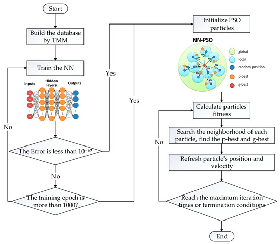
Figure 1.
The flow chart of NN-PSO.
A five-layer-film case is used to verify the NN-PSO method here. For the database of the forward NN in this case, the reflection spectra are calculated by using the transfer matrix method (TMM), which can be calculated using the following series of equations in the matrix form.
Here, k is the number of thin-film layers, Pi is the propagation matrix of the i-th layer, Ti,j is the transition matrix of the interface between layers i and j, which can be given as follows:
ni and di are the refractive index and thickness of layer i, respectively, and the reflectivity of the k-layer structure can be given by .
Here, the layer thicknesses can be limited to the following ranges: D1 = [147.7, 227.7], D2 = [130.4, 210.4], D3 = [366.1, 446.1], D4 = [192.1, 272.1], and D5 = [3.5, 43.5] (D1~D5 are the thicknesses of each layer, in nm). The spectrum is between 1~1.65 μm with a sampling grid of 5 nm for 131 points. The database contains 6498 samples, with 70% for training, 15% for testing, and 15% for validation. In addition, another 500 independent samples are reserved for the final test of the network. The mean square error (MSE) of the predicted spectra, in contrast to the desired one, is used as the loss function, with a target value of 10−6. The maximum number of epochs of NN training is 1000, the additional momentum factor is 0.9, and all other parameters are set to their default values [25,26]. Here, the network has 3 hidden layers (each layer contains 50 neurons), 5 inputs, and 131 outputs.
After training the forward NN, the PSO algorithm is used to carry out the inverse design. We search for the minimum MSE between the target spectrum and the one that is predicted by the neural network. The number of PSO particles is 24, the maximum number of iterations is 500, and the searching ranges of the particles are D1 = [100, 300], D2 = [100, 300], D3 = [300, 500], D4 = [200, 300], and D5 = [0, 100] (nm), respectively. The local and global acceleration factors are 2, and the termination condition is MSE less than 10−5, while all other parameters take their default values [33]. The CPU we used in this paper for the nano thin-film simulations is a Intel(R) Core (TM) i5-8500 processor with an NVIDIA GeForce GTX 1050 Ti GPU acceleration card. The software we used for this study are MATLAB and Python for the TMM and NN/PSO simulations, respectively.
3. Results and Discussion
The reflection spectra calculated by TMM and NN for one randomly selected sample from the test set are shown in Figure 2a, where we can see that the NN prediction is close to the TMM result for the whole wavelength range of 1000~1650 nm (especially for the 1400~1500 nm wavelengths of interest). To analyze the results more statistically, Figure 2b shows the error distribution histogram of the neural network prediction for the test dataset of 500 samples (each sample contains 131 wavelength points). It can be seen that the error of the neural network prediction is generally less than 0.04%, which indicates that it is highly consistent with the original spectra.
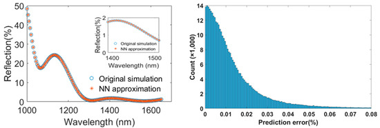
Figure 2.
(a) The reflection spectrum generated by TMM and NN, and (b) the error distribution of the NN prediction against the test dataset.
For this case, it took about 571 s to obtain a set of design parameters by the TMM-PSO method and 112 s by NN-PSO, which means that the inverse design of the multilayer thin-films by the NN-PSO method can greatly improve the simulation speed compared to TMM-PSO. The original parameter X = [189.22, 185.79, 388.76, 247.13, 41.48] and the error relative to the target spectrum can be minimized to 1.3 × 10⁻²%, as shown in Figure 3 for the NN-PSO optimization process.
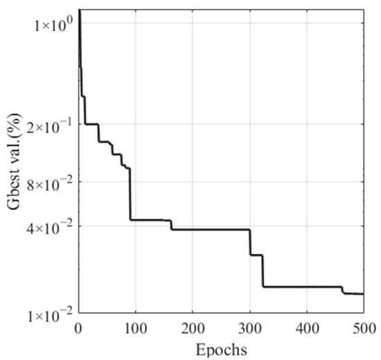
Figure 3.
The convergence curve of NN-PSO.
Table 1 lists the statistical results for 50 repeated inverse designs whose relative errors (RE) between their mean values and the original true ones are less than 3.45%, and the predicted thicknesses are within a 2 nm standard deviation (STD). The reflection spectrum for the mean values of the parameters predicted by NN-PSO was calculated using TMM to compare with the original spectrum, as shown in Figure 4a. It can be seen that the three spectra overlap with each other with high accuracy in the MSE histogram plotted in Figure 4b. Thus, the NN-PSO method can be used for the inverse design of the multilayer thin-films with high speed and accuracy in the parameter searching process.

Table 1.
The statistical results of inverse design for the AR coating case.
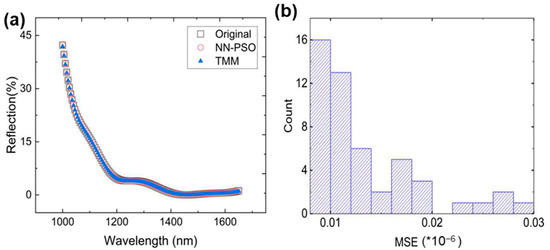
Figure 4.
(a) Reflection spectrum verification and (b) the MSE distribution histogram of NN-PSO predicted spectra.
Then, we truncated the 1400~1500 nm range of the original spectrum as a new target range to obtain multiple structures for the AR coating design. These structures are listed in Table 2, where TMM was used to generate the reflection spectrum for each structure and compared to the target one, as in Figure 5. It can be seen that the reflection spectra generated according to these structural parameters achieved high precision in the desired wavelength range, and the combination of the DLNN and PSO algorithm can map the design parameter space and tackle the single-solution problem of the tandem neural network [21].
Table 2.
The structures obtained by NN-PSO for AR coating in Figure 5.
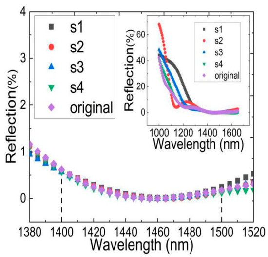
Figure 5.
The reflection spectra for various structures inversely designed by NN-PSO for the same 1400~1500 nm wavelength range.
4. Experiment Case
4.1. The Anti-Reflection (AR) Coating Case
To verify the application of the NN-PSO method in a real experiment, we used the reflection spectrum of a five-layer-AR film grown by the ion-beam-assisted coating system as an example, as in Figure 6a. The materials of the films on top of the fused silica substrate were SiO2 and Ta2O5, whose refractive indices were measured individually in their thin-film format, as shown in Figure 6b. In the experiment, the thicknesses were set to 255.88, 24.33, 28.85, 74.90, and 98.58 nm for the five layers (denoted by D1 to D5), respectively. Then, we grew the film by the e-beam heating of their solid sources such that SiO2 and Ta2O5 molecules could evaporate and escape from the source to be deposited on the substrate held at the top section of the coating machine, which rotated under a constant speed to ensure the uniformity of the deposition. The quartz crystal monitor was used to check the layer thickness, and the growth process was held under a low pressure of 10−6 Torr and a constant temperature of 150 °C. After growth, the thin-film was tested for its reflection spectrum, as shown in Figure 7a.
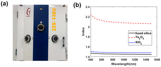
Figure 6.
(a) The ion-beam-assisted coating system and (b) the indices of the materials used in the thin-film growth.
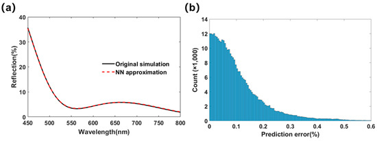
Figure 7.
(a) The predicted reflection spectrum by NN compared to TMM and (b) the error distributions for NN in the five-layer AR case.
Then, to evaluate the grown film quality and estimate the layer thickness inversely, we took the thickness ranges of D1 = [225.88, 285.88], D2 = [0, 300], D3 = [0, 300], D4 = [44.90, 104.90], and D5 = [68.58, 128.58] to generate the reflection spectrum database, as described in Section 2 for the forward network. There were 5 inputs and 351 outputs for the forward network, which had three hidden layers and 50 neurons for each. The database had 5000 samples (85% for training and 15% for testing), and the MSE for the test set (with 750 independent samples) as predicted by the NN was 2.36 × 10⁻⁶, and the error distribution is shown in Figure 7b.
Then, the trained NN was used by PSO to carry out the inverse design, as shown in Figure 8. Here, the number of particles was 20, the maximum number of PSO iterations was 50, and the curve obtained by the experiment was inversely analyzed 50 times. The experimental curve and the spectrum that was calculated by the TMM for the pre-set values and by TMM-PSO are given as the black solid, red dashed, and purple dotted lines, respectively, as in Figure 8a. There were some differences between those, and the spectrum from TMM-PSO (the purple line) was closer to the experimental curve (the black one) than the spectrum calculated by TMM (the red one), which may be due to the differences between the refractive index parameters used and the actual ones. The thicknesses of the grown thin-film layers also had some fluctuations compared to their pre-set values. The yellow dash-dotted line shows the least error for 50 inverse designs by NN-PSO, with an overall MSE of 5.31 × 10⁻⁶, as in Figure 8b. Here, the dash-asterisk lines are the results of D1 to D5, whose average values are 243.58, 18.17, 36.27, 76.58, and 98.99 nm, respectively. Then, the relative error of the predicted results as compared to the preset values (as marked by the solid lines) were 5.05, 33.90, 20.46, 2.19, and 0.41 (%), respectively. Here, D1 had the largest absolute error, and D2 and D3 had larger REs of the predicted results than the preset values. This may be because D1 was closest to the substrate and it may have had a larger error due to film monitoring during the initial growth, and D2 and D3’s larger REs were due to their relatively thinner thicknesses. The MSE distribution histogram of the NN-PSO predicted spectra is shown in Figure 8c, which shows that all of the MSEs of the spectra were less than 6 × 10⁻⁵, with most of them being less than 2 × 10⁻⁵. Therefore, it can be considered that the inverse result is accurate.
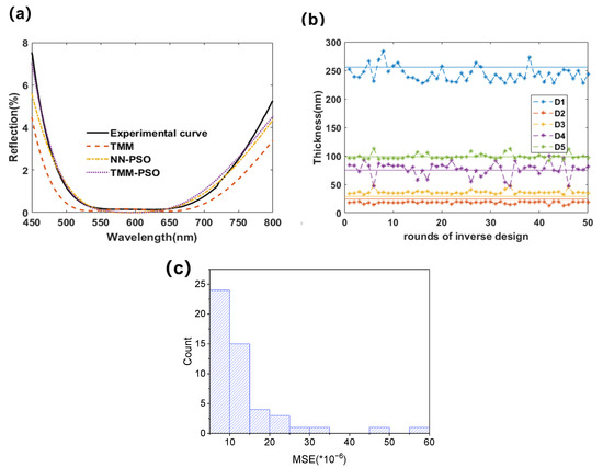
Figure 8.
(a) The reflection curves as compared to the experiment, TMM and NN-PSO, (b) the distribution of the NN-PSO inversely designed layer thicknesses, and (c) the MSE distribution histogram of NN-PSO predicted spectra.
We also compared it with the TMM-PSO method, which uses the transfer matrices directly without training an NN beforehand to work with PSO for the inverse design. For this case, it took 233 s and 595 s for each design round of NN- and TMM-PSO, respectively. If the database collection and training time for the former is also included, it would take 760 s for the NN-PSO method. However, since the NN itself is cumulative and can summarize/map the whole parameter space comprehensively, we can therefore obtain a surrogate model for the studied system for later repeated use and immediate reference at any time. For example, in the 50 rounds of the PSO inverse design processes, TMM-PSO kept calculating using TMM and could be about 50 times more time-consuming than NN, due to the latter one’s direct citation of the surrogate network in the 2nd~50th rounds of NN-PSO processes. Therefore, NN-PSO has great advantages and high accuracy in data analysis and easier citation for future accumulated expansion/improvement.
In order to obtain more structures with high transmittance between 550 and 650 nm, as previously conducted in the simulation case, as in Figure 5, the experimental spectrum in this range was also used as the new target for NN-PSO to use the inverse design, where a variety of structures can be obtained, as listed in Table 3. TMM was used to verify the reflection spectrum for each inversely designed structure compared to the target, as in Figure 9. The results show that NN-PSO can obtain multiple designs for the same spectrum, which can be used for parameter extraction and failure analysis applications.
Table 3.
The structures obtained by NN-PSO for the same spectrum in range of 550~650 nm.
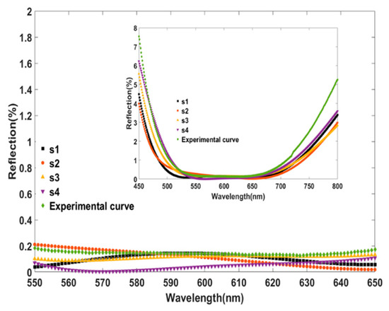
Figure 9.
The reflection spectra of various structures inversely designed for the 550~650 nm wavelength range.
4.2. Bragg Case
To test the robustness of our method for more challenging cases, such as the Bragg structure, which has more oscillation peaks/valleys in the spectra, we can use a larger database to conduct the network training. Here, the tested Bragg structure had 34 layers of the materials SiO2 and Ta2O5 on top of the BK7 substrate. For periodic even (odd) layers, we can use only two thickness parameters to characterize the film, i.e., D1 for the SiO2 layers and D2 for the Ta2O5 layers. The output parameter of the network is the transmission spectrum, whose wavelength range is 400~1500 nm, with a total number of 1101 sampling points for 1 nm spacing. The refractive indices of the materials used in the experiment were the same as in the AR film, as shown in Figure 6b, whose film thicknesses for growth were preset to 179.57 nm (SiO2) and 126.43 nm (Ta2O5), respectively. Then, we could take [179.57 − 30, 179.57 + 30] nm (SiO2) and [126.43 − 30, 126.43 + 30] (Ta2O5) as the input parameter ranges to generate transmission spectra for the training database of our deep learning neural network.
The forward NN, denoted by NN1 here, had 4 hidden layers (each layer contained 100 neurons), 2 inputs, and 1101 outputs, and its database contained 20,000 samples (85% for training and 15% for testing). The MSE of the spectra predicted by NN1 was 7.0284 × 10⁻⁴, as verified against the test set.
Furthermore, if we consider the actual nano-coating process, where thicknesses for the top and bottom layers may sometimes be more difficult to be controlled in the experiment compared to the other layers, we can use six structural parameters D1 to D6 as the input data to train a different forward NN (denoted by NN2). Here, D1, D2, D5, and D6 represent the thicknesses of the 1st, 2nd, 33rd, and 34th layer, and D3 and D4 are the thicknesses of the other odd and even layers, respectively. The number of the neurons in each hidden layer of NN2 was 100, 500, 1000, 1000, 1000, and 500, respectively. The database contained 20000 samples (85% for training and 15% for testing) and the final MSE was 11.6336 × 10⁻⁴. The prediction results and error distributions of the two NNs are shown in Figure 10a,b, respectively.
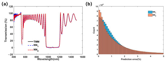
Figure 10.
(a) The predicted spectra compared to the original one that was randomly selected from the training dataset and (b) the error distributions for the two NNs.
Then, the trained NN can be used in PSO to find the layer thicknesses corresponding to the experimental spectrum. Here, the PSO searching ranges for the layer thicknesses were the same as the forward NN. For NN1, the number of particles was 20, the maximum number of iterations was 50, and the experimental curve accumulated 25 inverse designs, whose distribution is shown in Figure 11a. It can be seen that the predicted thicknesses were generally around 178.20 nm for SiO2 and 127.73 nm for Ta2O5, which were the mean values of the samples close to the growth values of 179.57 nm (SiO2) and 126.43 nm (Ta2O5), i.e., with REs of 0.77% (SiO2) and 1.03% (Ta2O5) for NN1-PSO. For NN2, the number of PSO particles was 60, the maximum number of iterations was 50, the repeated time of inverse designs was 25, and the distribution of the results is shown in Figure 11b. It can be seen that the results of D3 and D4 were close to 178.66 and 127.14 nm (with REs of 0.51% and 0.56%), while the other four parameters had large fluctuations. This may be because D3 and D4 represent the majority of the thickness of the Bragg layers except for the top and bottom ones. Thus, these two parameters affect the spectrum more than the others. Moreover, this indicates that the Bragg structure is relatively robust against variations in the individual layers, such that even if the top and bottom layers fluctuate heavily, the spectrum still keeps its main shape.
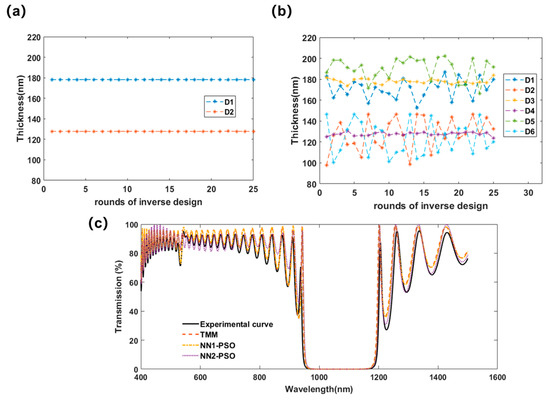
Figure 11.
(a,b) The result distribution statistics for the two NNs, and (c) the transmission spectra from the experimental measurement, from TMM simulation for the preset grown structure, and from NN1(/2)-PSO’s predictions.
To further verify the results, transmission curves generated by TMM, which used the pre-set growth parameters and the inversely designed ones, are shown in Figure 11c. The black solid line represents the measured experimental transmission spectrum of the films, the red dashed one was calculated by TMM using the preset growth values, and the yellow dash-dotted and purple dotted ones were generated for the mean values obtained from NN-PSO. Here, the MSE of NN1-PSO was 62.9927 × 10⁻⁴, and the MSE of NN2-PSO was 65.0205 × 10⁻⁴, which is still of high accuracy, considering the large fluctuations in the curves.
In order to test the multi-solution ability for the desired wavelength range, we narrowed the experimental curve to 950~1200 nm as the new inverse design target, as performed in the previous cases. The obtained structures are listed in Table 4, and their transmission spectrums generated by TMM are shown in Figure 12.
Table 4.
The structures obtained by NN-PSO for the Bragg case in Figure 12.
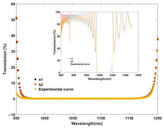
Figure 12.
The transmission spectra for various structures in the range of 950~1200 nm.
From the above comparisons, we can see that the NN-PSO method has high prediction accuracy and can be used in the experimental situations for complex spectra. The inverse designs for both the five-layer-film AR and Bragg experimental cases were verified. Multiple structures can be found for the same spectrum, if parameter-extraction or failure analysis are desired for that specific wavelength range.
5. Conclusions
The inverse design of nano thin-film coatings were tested using the high-precision and high-speed NN-PSO method, such that the single-solution problem of the tandem neural network could be solved. A five-layer-film AR case and a Bragg experimental one were used to verify the feasibility of this method for practical applications. In the AR coating case, the results indicate that the thicknesses of the grown layers may have some slight differences compared to the pre-set growth values for D2 and D3. In the Bragg case, two NNs were used to inversely design the structure with two and six structural parameters, which showed high accuracy, speed, and robustness. This indicates that it may be widely used in the inverse design of photonic devices and metamaterials as well as for practical cases in the optoelectronic industry. Photonic integrated circuits and optical device systems could be the next step, as we have been working on the ENN and FENN previously in order to extend the NN method to more complicated photonic devices for design parameter extractions as well as automatic AI designs. During the application of this method to practical/industry cases, one may experience long waiting times to accumulate experimental data, so the well-documented and comprehensive data collection and preparation could be highly important to balance the actual cost for this method to be successfully adopted.
Author Contributions
Conceptualization and methodology, Y.L.; validation, X.G. and J.L. (Jinsu Lu); resources, Y.L. and J.L. (Jianhong Li); writing—original draft preparation, X.G. and J.L. (Jinsu Lu); writing—review and editing, Y.L. and X.G.; supervision, Y.L.; funding acquisition, W.H. All authors have read and agreed to the published version of the manuscript.
Funding
This research was funded by National Key Research and Development Program of China (2018YFA0209000).
Data Availability Statement
Data are available upon reasonable request.
Conflicts of Interest
The authors declare no conflict of interest. The funders had no role in the design of the study; in the collection, analyses, or interpretation of data; in the writing of the manuscript; or in the decision to publish the results.
References
- Froemming, N.S.; Henkelman, G. Optimizing core-shell nanoparticle catalysts with a genetic algorithm. J. Chem. Phys. 2009, 131, 234103. [Google Scholar] [CrossRef]
- Piche, S.W. Steepest Descent Algorithms for Neural-Network Controllers and Filters. IEEE Trans. Neural Netw. 1994, 5, 198–212. [Google Scholar] [CrossRef]
- Ahmad, N.A. A Globally Convergent Stochastic Pairwise Conjugate Gradient-Based Algorithm for Adaptive Filtering. IEEE Signal Proc. Lett. 2008, 15, 914–917. [Google Scholar] [CrossRef]
- Malkiel, I.; Mrejen, M.; Nagler, A.; Arieli, U.; Wolf, L.; Suchowski, H. Plasmonic nanostructure design and characterization via Deep Learning. Light Sci. Appl. 2018, 7, 60. [Google Scholar] [CrossRef]
- Chen, Y.S.; Zhu, J.F.; Xie, Y.N.; Feng, N.X.; Liu, Q.H. Smart inverse design of graphene-based photonic metamaterials by an adaptive artificial neural network. Nanoscale 2019, 11, 9749–9755. [Google Scholar] [CrossRef]
- Elsawy, M.M.R.; Lanteri, S.; Duvigneau, R.; Briere, G.; Mohamed, M.S.; Genevet, P. Global optimization of metasurface designs using statistical learning methods. Sci. Rep. 2019, 9, 17918. [Google Scholar] [CrossRef]
- Du, Q.; Zhang, Q.; Liu, G.H. Deep learning: An efficient method for plasmonic design of geometric nanoparticles. Nanotechnology 2021, 32, 505607. [Google Scholar] [CrossRef]
- Guo, X.H.; Xu, X.P.; Li, Y.; Huang, W.P. Extendable neural network and flexible extendable neural network in nanophotonics. Opt. Commun. 2022, 508, 127671. [Google Scholar] [CrossRef]
- Baxter, J.; Lesina, A.C.; Guay, J.M.; Weck, A.; Berini, P.; Ramunno, L. Plasmonic colours predicted by deep learning. Sci. Rep. 2019, 9, 8074. [Google Scholar] [CrossRef] [Green Version]
- Asano, T.; Noda, S. Iterative optimization of photonic crystal nanocavity designs by using deep neural networks. Nanophotonics 2019, 8, 2243–2256. [Google Scholar] [CrossRef]
- Chugh, S.; Gulistan, A.; Ghosh, S.; Rahman, B.M.A. Machine learning approach for computing optical properties of a photonic crystal fiber. Opt. Express 2019, 27, 36414–36425. [Google Scholar] [CrossRef] [Green Version]
- Makarenko, M.; Burguete-Lopez, A.; Getman, F.; Fratalocchi, A. Generalized Maxwell projections for multi-mode network Photonics. Sci. Rep. 2020, 10, 9038. [Google Scholar] [CrossRef] [PubMed]
- Ding, F.; Bozhevolnyi, S.I. A Review of Unidirectional Surface Plasmon Polariton Metacouplers. IEEE J. Sel. Top. Quantum Electron. 2019, 25, 4600611. [Google Scholar] [CrossRef] [Green Version]
- Gu, G.H.; Noh, J.; Kim, I.; Jung, Y. Machine learning for renewable energy materials. J. Mater. Chem. A 2019, 7, 17096–17117. [Google Scholar] [CrossRef]
- Pun, G.P.P.; Batra, R.; Ramprasad, R.; Mishin, Y. Physically informed artificial neural networks for atomistic modeling of materials. Nat. Commun. 2019, 10, 2339. [Google Scholar] [CrossRef]
- So, S.; Mun, J.; Rho, J. Simultaneous Inverse Design of Materials and Structures via Deep Learning: Demonstration of Dipole Resonance Engineering Using Core-Shell Nanoparticles. ACS Appl. Mater. Interfaces 2019, 11, 24264–24268. [Google Scholar] [CrossRef]
- Raju, L.; Lee, K.T.; Liu, Z.C.; Zhu, D.Y.; Zhu, M.L.; Poutrina, E.; Urbas, A.; Cai, W.S. Maximized Frequency Doubling through the Inverse Design of Nonlinear Metamaterials. ACS Nano 2022, 16, 3926–3933. [Google Scholar] [CrossRef]
- An, S.S.; Zheng, B.W.; Julian, M.; Williams, C.; Tang, H.; Gu, T.; Zhang, H.L.; Kim, H.J.; Hu, J.J. Deep neural network enabled active metasurface embedded design. Nanophotonics 2022. [Google Scholar] [CrossRef]
- Dai, P.; Sun, K.; Yan, X.Z.; Muskens, O.L.; de Groot, C.H.; Zhu, X.P.; Hu, Y.Q.; Duan, H.G.; Huang, R.M. Inverse design of structural color: Finding multiple solutions via conditional generative adversarial networks. Nanophotonics 2022, 11, 3057–3069. [Google Scholar] [CrossRef]
- Qiu, C.K.; Wu, X.; Luo, Z.; Yang, H.D.; Huang, B. Fast inverse design of nanophotonics using differential evolution back-propagation. Opt. Commun. 2022, 514, 128155. [Google Scholar] [CrossRef]
- Xu, X.P.; Sun, C.L.; Li, Y.; Zhao, J.; Han, J.L.; Huang, W.P. An improved tandem neural network for the inverse design of nanophotonics devices. Opt. Commun. 2021, 481, 126513. [Google Scholar] [CrossRef]
- Liu, D.J.; Tan, Y.X.; Khoram, E.; Yu, Z.F. Training Deep Neural Networks for the Inverse Design of Nanophotonic Structures. ACS Photonics 2018, 5, 1365–1369. [Google Scholar] [CrossRef] [Green Version]
- Mortazavifar, S.L.; Salehi, M.R.; Shahraki, M.; Abiri, E. Ultra-thin broadband solar absorber based on stadium-shaped silicon nanowire arrays. Front. Optoelectron. 2022, 15, 6. [Google Scholar] [CrossRef]
- Xing, X.J.; Guo, J.W.; Nan, L.L.; Gu, Q.Y.; Zhang, X.P.; Yan, D.M. Efficient MSPSO Sampling for Object Detection and 6-D Pose Estimation in 3-D Scenes. IEEE Trans. Ind. Electron. 2022, 69, 10281–10291. [Google Scholar] [CrossRef]
- Ma, Z.H.; Feng, P.; Li, Y. Inverse design of semiconductor laser parameters based on deep learning and particle swarm optimization method. Proc. SPIE 2019, 11209, 112092X. [Google Scholar] [CrossRef]
- Ma, Z.H.; Li, Y. Parameter extraction and inverse design of semiconductor lasers based on the deep learning and particle swarm optimization method. Opt. Express 2020, 28, 21971–21981. [Google Scholar] [CrossRef] [PubMed]
- Ong, J.R.; Chu, H.S.; Chen, V.H.J.; Zhu, A.Y.T.; Genevet, P. Freestanding dielectric nanohole array metasurface for mid-infrared wavelength applications. Opt. Lett. 2017, 42, 2639–2642. [Google Scholar] [CrossRef] [Green Version]
- Gonzalez-Alcalde, A.K.; Salas-Montiel, R.; Mohamad, H.; Morand, A.; Blaize, S.; Macias, D. Optimization of all-dielectric structures for color generation. Appl. Opt. 2018, 57, 3959–3967. [Google Scholar] [CrossRef]
- Barreda, A.; Albella, P.; Moreno, F.; Gonzalez, F. Broadband Unidirectional forward Scattering with High Refractive Index Nanostructures: Application in Solar Cells. Molecules 2021, 26, 4421. [Google Scholar] [CrossRef]
- Manko, V.A.; Manko, A.A.; Sukach, G.A. Method of calculation of multilayer optical filters using thin films. In Proceedings of the 2006 International Workshop on Laser and Fiber-Optical Networks Modeling, Kharkiv, Ukraine, 29 June–1 July 2006; pp. 452–454. [Google Scholar]
- Peurifoy, J.; Shen, Y.C.; Jing, L.; Yang, Y.; Cano-Renteria, F.; DeLacy, B.G.; Joannopoulos, J.D.; Tegmark, M.; Soljacic, M. Nanophotonic particle simulation and inverse design using artificial neural networks. Sci. Adv. 2018, 4, eaar4206. [Google Scholar] [CrossRef] [Green Version]
- Lenaerts, J.; Pinson, H.; Ginis, V. Artificial neural networks for inverse design of resonant nanophotonic components with oscillatory loss landscapes. Nanophotonics 2021, 10, 385–392. [Google Scholar] [CrossRef]
- Trelea, I.C. The particle swarm optimization algorithm: Convergence analysis and parameter selection. Inf. Process. Lett. 2003, 85, 317–325. [Google Scholar] [CrossRef]
Publisher’s Note: MDPI stays neutral with regard to jurisdictional claims in published maps and institutional affiliations. |
© 2022 by the authors. Licensee MDPI, Basel, Switzerland. This article is an open access article distributed under the terms and conditions of the Creative Commons Attribution (CC BY) license (https://creativecommons.org/licenses/by/4.0/).