Ultracompact Deep Neural Network for Ultrafast Optical Property Extraction in Spatial Frequency Domain Imaging (SFDI)

Abstract

Spatial frequency domain imaging (SFDI) is a powerful, label-free imaging technique capable of the wide-field quantitative mapping of tissue optical properties and, subsequently, chromophore concentrations. While SFDI hardware acquisition methods have advanced towards video-rate, the inverse problem (i.e., the mapping of acquired diffuse reflectance to optical properties) has remained a bottleneck for real-time data processing and visualization. Deep learning methods are adept at fitting nonlinear patterns, and may be ideal for rapidly solving the SFDI inverse problem. While current deep neural networks (DNN) are growing increasingly larger and more complex (e.g., with millions of parameters or more), our study shows that it can also be beneficial to move in the other direction, i.e., make DNNs that are smaller and simpler. Here, we propose an ultracompact, two-layer, fully connected DNN structure (each layer with four and two neurons, respectively) for ultrafast optical property extractions, which is 30×–600× faster than current methods with a similar or improved accuracy, allowing for an inversion time of 5.5 ms for 696 × 520 pixels. We further demonstrated the proposed inverse model in numerical simulations, and comprehensive phantom characterization, as well as offering in vivo measurements of dynamic physiological processes. We further demonstrated that the computation time could achieve another 200× improvement with a GPU device. This deep learning structure will help to enable fast and accurate real-time SFDI measurements, which are crucial for pre-clinical, clinical, and industrial applications.

1. Introduction

Tissue optical properties (OPs), including the absorption coefficient (µ_a) and the reduced scattering coefficient (µ_s′), carry important physiological information about tissue structure, composition, and function. The reduced scattering coefficient reflects the size and size distribution of tissue scattering components on the cellular and sub-cellular levels. The absorption coefficient is associated with the number of light-absorbing species in biological tissue. Further, with absorption measured at different wavelengths, the concentration of primary light-absorbing molecules, such as oxy- and deoxy-hemoglobin, can be quantitatively resolved by solving a matrix equation (i.e., Beer’s Law) [1].

Spatial Frequency Domain Imaging (SFDI) is an emerging label-free imaging technique that provides quantitative tissue optical properties (µ_a and µ_s′) on a pixel-by-pixel basis in a wide-field format [2,3]. SFDI is being applied to an increasing number of biomedical scenarios, including animal imaging, burn wound monitoring, clinical tissue flap monitoring, and others [4,5,6,7,8,9,10]. The details of SFDI image acquisition and data processing will be illustrated in the Methods section. In brief, a series of spatially modulated light patterns are projected onto the tissue, and a camera collects remitted light. The use of two carefully selected spatial frequencies (such as 0 and 0.1 mm⁻¹) allows for the separation of tissue absorption and scattering [4]. The collected images are demodulated and calibrated against a tissue-mimicking phantom with known optical properties (OPs) to obtain diffuse reflectance at each spatial frequency, denoted as R_d (f_x). The R_d pair is then fed into an inverse model, which is used to extract µ_a and µ_s′ in a pixel-by-pixel manner for each illumination wavelength. The extracted µ_a of multiple wavelengths can be used to calculate tissue chromophore concentrations using Beer’s Law.

A current goal of SFDI method development is the rapid and accurate quantification of tissue OPs and chromophore components with real-time feedback. This would facilitate point-of-care decision-making in a wide-variety of clinical settings. Recent improvements in SFDI hardware acquisition have advanced data capturing towards video-rate [11,12]. After image acquisition, both demodulation and calibration can be implemented as rapid matrix-based operations in Matlab. A current data-processing bottleneck lies in the conversion of the R_d values to optical properties, which must occur for each pixel within the image. Prior methods have utilized iterative minimization algorithms and look-up-tables (LUTs) to solve the inverse problem [3,13]. For this work, we explored the use and design of deep learning inverse models that accept the R_d pair (0 and 0.1 mm⁻¹) as input, and directly output µ_a and µ_s′. We note that deep neural networks (DNNs) are those that have two or more layers [14]. This is in contrast to traditional, one-layer, shallow-structure networks. The power of deep learning partially lies in its ability to fit nonlinear patterns [15], implying that it may be ideal for SFDI inverse problems.

Single-layer neural networks have previously been applied to estimations of the optical properties of two-layer media [16], and several other works have applied deep neural networks to address the inverse problem for optical properties in the field of diffuse optics [17,18,19]. For example, prior deep learning work has used multi- f_x (>2 modulation frequencies) for SFDI, with the intent of identifying a model with maximum accuracy based on the large collected datasets [17,20]. In contrast, this work is focused on the much more common scenario of 2- f_x SFDI, with optimization directed towards the most compact structure while maintaining high accuracy. This optimization is potentially beneficial under two scenarios: 1. in the case of rapid real-time feedback, where speed is of the utmost importance, and 2. in the case where computing hardware is limited. The simple network structure here can easily be implemented using standard PC’s, or even on a microprocessor. This makes it ideal for low-cost applications where higher-end computing hardware is not available. While current deep learning models tend to grow increasingly larger and more complex (e.g., millions of parameters or even more for U-Net), here, we move in the opposite direction, proposing a smaller and simpler deep-learning model that achieves both high speed and accuracy. The simplicity of our approach also differentiates the proposed model from other recent work using parallel computing architecture with graphical processing units (GPUs) [21]. Additionally, we also demonstrate how the network topology affects the tradeoffs between accuracy and speed, which are little mentioned in the prior literature.

2. Methods

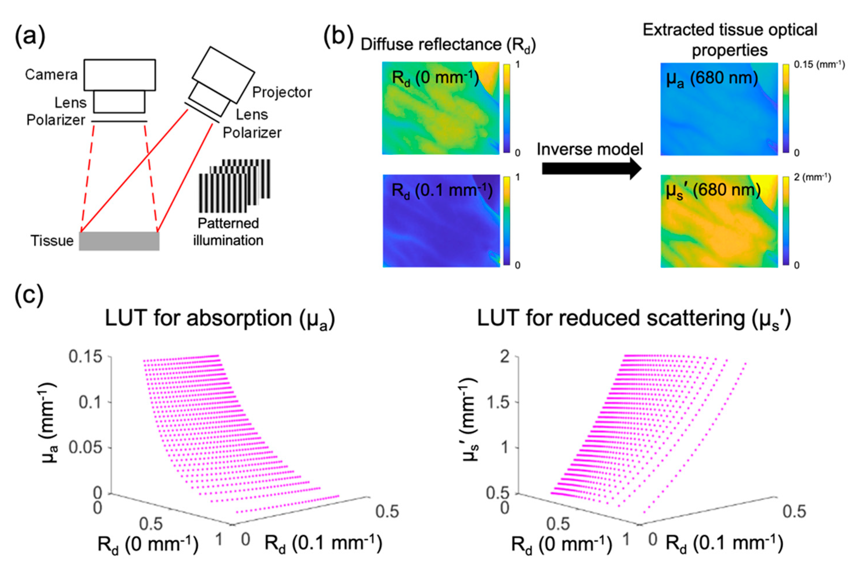
SFDI image acquisition and data processing are illustrated in Figure 1. Figure 1a shows the SFDI instrument. A series of spatially modulated light patterns (shifted 120° sequentially in phase) were projected onto the sample, and a camera collected the remitted light. The use of two carefully selected spatial frequencies (such as 0 and 0.1 mm⁻¹) allows for the separation of tissue absorption and scattering [4]. To obtain the spatial frequency response of the samples at 0 and 0.1 mm⁻¹, the images collected from the phantom (with known OPs) and the tissue (with unknown OPs) were demodulated with Equations (1) and (2), respectively, whereas $I_1$, $I_2$ and $I_3$ denote the raw images of different phases. The demodulated maps of the tissue were then calibrated against those of the phantom using Equation (3) to obtain diffuse reflectance (R_d) maps at the two spatial frequencies. R_d and I refer to diffuse reflectance and demodulation maps, respectively, and subscripts tis and ref refer to the tissue and calibration phantom, respectively. Note that the demodulation and calibration can both be implemented as rapid matrix-based operations. As shown in Figure 1b, the consequent R_d maps are then fed into an inverse model, such as the Monte Carlo Look-Up-Table (LUT), which is used to extract µ_a and µ_s′ in a pixel-by-pixel manner for each illumination wavelength (there are two Monte Carlo LUTs, mapping the R_d values to µ_a and µ_s′ respectively). The Monte Carlo LUTs for µ_a and µ_s′ are visualized in Figure 1c. The extracted µ_a of multiple wavelengths can be used to calculate tissue chromophore concentrations using Beer’s Law. Note that the mapping from R_d to OPs represents the bottleneck for optical property extraction.

$$I\left(f_x=0 m{m}^{-1}\right)=\frac{I_1+I_2+I_3}{3}$$

(1)

$$I\left(f_x=0.1 m{m}^{-1}\right)=\frac{\sqrt{2}}{3}\sqrt{\left({\left(I_1-I_2\right)}^2+{\left(I_2-I_3\right)}^2+{\left(I_3-I_1\right)}^2\right)}$$

(2)

$$R_{d,tis}\left(f_x\right)=\frac{I_{tis}\left(f_x\right)}{I_{ref}\left(f_x\right)}{R}_{d,ref}\left(f_x\right)$$

(3)

To address the bottleneck of OP extraction, we systematically explored the hyperparameter space as well as three commonly used activation functions, and compared the speed and accuracy of the corresponding DNNs. Specifically, we investigated the tradeoffs between speed and accuracy for different numbers of neural layers (number of layers: 1, 2, 4, 6, and 8), and numbers of neurons in each layer (number of neurons: 2, 4, 6, 8, and 10). The three activation functions that we explored were tanh, sigmoid, and softsign [22,23,24]. We also tested ReLU activation function, which, as expected, was not able to provide an accurate OP prediction under small network structures due to its “semi-linear” nature (data not shown) [15]. The DNNs were trained with different combinations of these hyperparameters and activation functions, and tested for speed and accuracy. The training data were generated for a wide range of OPs using an established “white” Monte Carlo model [25], with µ_a sampled from 0.001 mm⁻¹ to 0.15 mm⁻¹ in 0.001 mm⁻¹ increments, and µ_s′ sampled from 0.51 mm⁻¹ to 2 mm⁻¹ with 0.01 mm⁻¹ increments, using 0 and 0.1 mm⁻¹ spatial frequencies. The training data had 150 × 150 OP pairs. Hyperparameters were tuned in Keras with TensorFlow as a backend [26]. The Adam optimization algorithm was used with an initial learning rate of 0.001 and batch size of 128 [27]. The mean squared error was minimized as a loss function, and the training took approximately half an hour on the CPU. The trained models were implemented as a Matlab function to facilitate comparisons of speed and accuracy. For the test data, 10,000 OP combinations were randomly selected in the range of [0.001, 0.15] mm⁻¹ for µ_a and [0.51, 2] mm⁻¹ for µ_s′, and the corresponding R_d values were generated using the MC forward model.

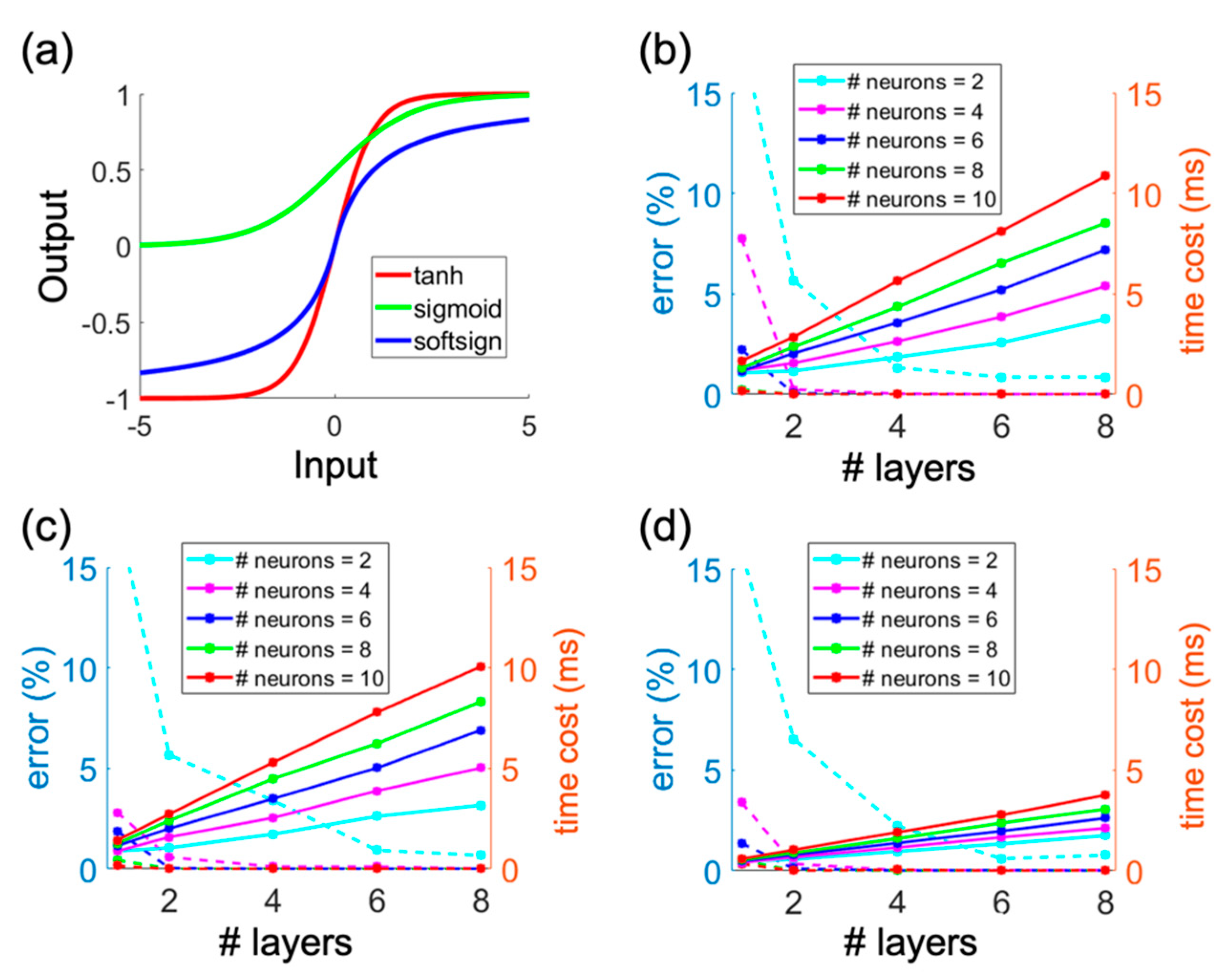
The three different activation functions are shown in Figure 2a. Figure 2b provides a comparison of the speed and accuracy performance of the DNNs using the tanh activation function. Note that the accuracy performance was characterized by the standard deviation of percent errors calculated from both µ_a and µ_s′ simultaneously; errors had minimal bias. The solid lines in Figure 2b represent the average time cost (repeated 10 times) for processing the 10,000 optical property inversions in the test data. The plots show that higher time costs are incurred as more neurons are added to each layer or when the number of layers is increased. The dashed lines in Figure 2b show optical property inversion errors. The plot shows that increasing the number of neurons in each layer, or the total number of layers, both lead to more accurate inversions. Importantly, the plot shows that there are diminishing returns in accuracy improvements as the number of layers increases past a certain point. This point is dependent on the number of neurons utilized per layer. Figure 2c,d show the results for the other activation functions, all of which show similar trends. When two or more layers were utilized, the three different activation functions had a similar accuracy performance. However, there was a large difference in speed among the activation functions, and DNNs utilizing the softsign activation function were faster than DNNs using the tanh and sigmoid functions. This is because the softsign function can be implemented as a matrix operation, whereas the tanh and sigmoid both have exponential terms, which are slower to compute. Overall, the exploration of hyperparameters and activation functions in Figure 2 demonstrates that DNNs that utilize the softsign activation function with 2 layers, and 4 neurons in each layer, provide a combination of fast optical property inversions with high accuracy. Increasing the number of layers or neurons above these levels provided only marginal improvements in accuracy.

To date, we have demonstrated the identification of the deep neural network for SFDI inverse problem with exploration of hyperparameters and activation functions as well as the corresponding tradeoffs regarding speed and accuracy.

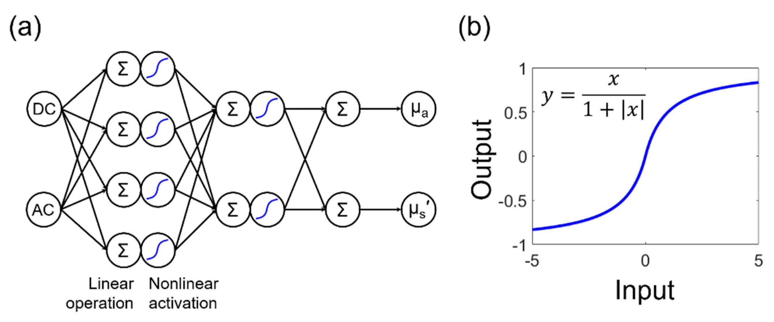
Based on these results, we further tuned the DNN structure to be even more efficient, with a simpler structure of two hidden layers, with 4 neurons in the first layer and 2 neurons in the second layer. This DNN structure is shown in Figure 3a. The softsign activation function and its formulation are demonstrated again in Figure 3b. This function is nonlinear and maps data from (−∞, +∞) to (−1, 1). This model’s code is available in a GitHub repository [28].

The optimized DNN structure with softsign activation was compared to two prior inversion methods based on look-up-tables (LUTs). The first method utilizes interpolation of the R_d vector within a LUT that maps R_d values to OPs [3]. LUTs using this method are generated by linearly sampling the OP space. Therefore, we refer this method as the “linear OP LUT”. For this method, as the sampling density is increased, OP extraction accuracy increases at the expense of computational time. More recently, a modified method was developed that rounds measured R_d values to the closest LUT entry, effectively performing a direct search of the LUT [13]. This improves speed as it avoids interpolation. The LUTs for this method are generated by linear sampling in the R_d space [13]. Therefore, we will refer to this method as the “linear R_d LUT”. For this work, all LUTs were generated using results from a “white” Monte Carlo (MC) forward model [25]. Both the linear OP LUT and linear R_d LUT were 150 × 150, which is the same dimension as the DNN training data. The linear OP LUT was constructed using the exact same data that were used to train the DNN. The linear R_d LUT was constructed by linearly sampling the R_d space in the range of [0, 1]. The linear OP LUT interpolation was implemented using the “griddata” function in Matlab [3]. The linear R_d LUT method was also implemented in Matlab, as described in previous work [13]. The computations of speed and accuracy comparisons were conducted on a desktop computer with an Intel i9-9900K CPU and 64 GB of RAM.

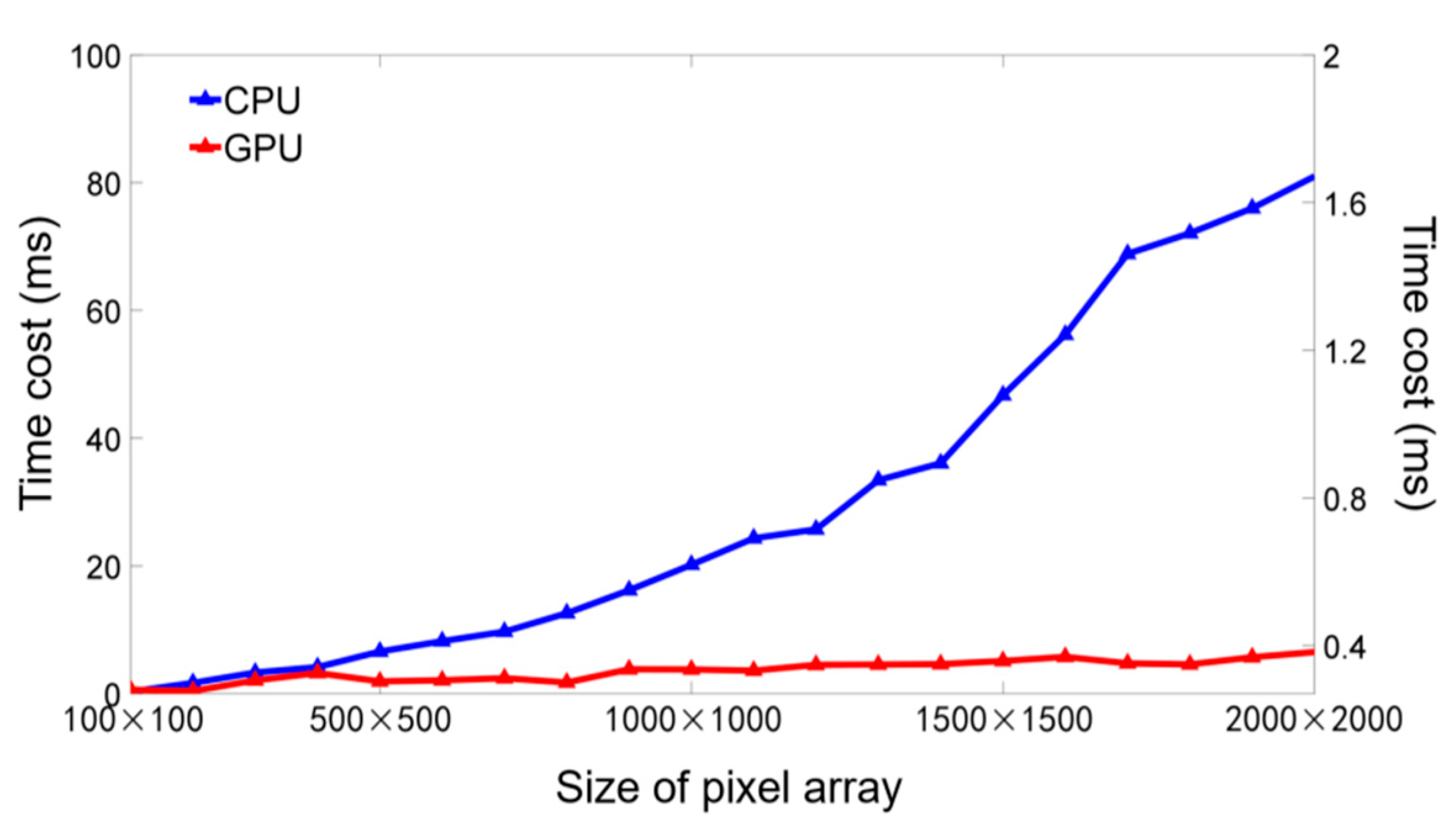
While GPUs have been extensively used to accelerate computations, we further tested the proposed DNN for optical property inversions on a desktop computer equipped with a typical GPU device (NVIDIA GeForce RTX 3070). Different sizes of pixel array were used in the test, ranging from 100 × 100 to 2000 × 2000 pixels. The inversions were repeated 100 times for each pixel array size to reduce randomness. The inversions were also conducted using the CPU (Intel i7-7700K) on the same desktop to obtain a sense of the differences in speed between CPU and GPU devices. In addition, the time cost with GPU was recorded using the NVIDIA Nsight environment.

Finally, we demonstrated applications, including in phantom validation and in vivo measurements of the human hand. In the phantom validation study, a total of nine phantoms with a wide range of optical absorption and scattering properties were fabricated using nigrosin (N814749-100g, Macklin, Shanghai, China), titanium dioxide (TiO2) (PL975541-500g, Cool Chemistry, Beijing, China), silicone base and its curing agent (#906, Chunlan, Meizhou, China). For in vivo measurements, human tissue imaging was conducted on the back of the hand of a healthy volunteer. The experimental procedures were reviewed and approved by the Beihang University Biological and Medical Ethics Committee.

3. Results

For accuracy comparisons, 10,000 OP combinations were randomly selected in the range of [0.001, 0.15] mm⁻¹ for µ_a and [0.51, 2] mm⁻¹ for µ_s′, and the corresponding R_d values were generated using the MC-forward model. Gaussian random noise of zero-mean and standard deviations of 0%, 1%, and 2% was added to the R_d data, and the optical property extractions were conducted using the above methods. The mean and standard deviation of the percent errors for µ_a and µ_s′ are compared in

Table 1. Comparison of accuracy of optical property extractions for Look-Up-Table (LUT) and Deep Neural Network (DNN) inversion models.

	Percent Error
	Linear OP LUT		Linear Rd LUT		DNN
	µa	µs′	µa	µs′	µa	µs′
0% noise	0.0 ± 1.5%	0.0 ± 0.48%	−1.1 ± 2.5%	0.5 ± 1.7%	0.0 ± 1.4%	0.0 ± 0.28%
1% noise	0.0 ± 4.1%	0.0 ± 2.0%	−1.1 ± 4.5%	0.5 ± 2.5%	0.1 ± 4.2%	0.0 ± 2.0%
2% noise	0.2 ± 7.6%	0.0 ± 3.8%	−1.1 ± 7.8%	0.4 ± 4.1%	0.4 ± 8.0%	0.2 ± 4.1%

for the three methods. In general, the linear OP LUT method had a lower mean and standard deviation errors compared to the linear R_d LUT method. This is expected, as the linear OP LUT utilizes interpolation, whereas the linear R_d LUT method outputs OP values directly from the pre-computed LUT. The DNN achieved comparable accuracy to the linear OP LUT method for both µ_a and µ_s′ extractions.

The computational speed was compared between the three inversion methods by generating OP arrays of sizes 100 × 100 and 696 × 520 pixels (full image size after 2 × 2 binning in previously published SFDI systems) [9,10]. OPs were randomly generated as before. Inversions for each case were repeated 10 times.

Table 2. Comparison of speed for the inversions from R_d to OPs.

# Datapoints	Linear OP LUT (ms)	Linear Rd LUT (ms)	DNN (ms)
100 × 100	124.8 ± 2.6	5.7 ± 0.4	0.2 ± 0.03
696 × 520	1249.6 ± 7.2	212.7 ± 4.0	5.5 ± 0.2

shows speed comparisons. For the 100 × 100 pixels R_d maps (i.e., 10,000 inversions from R_d to OPs), the linear OP LUT took approximately 125 ms on average, and the linear R_d LUT took approximately 6 ms. In comparison, the DNN only took 0.2 ms. With a full-sized image of 696 × 520 pixels, the inversion process took over 1.2 s for the linear OP LUT, and approximately 210 ms for the linear R_d LUT, respectively. In contrast, the proposed DNN inverse model took only 5.5 ms. In both cases, the DNN was approximately 30–40 times faster than the linear R_d LUT method, and over 200–600 times faster than the linear OP LUT.

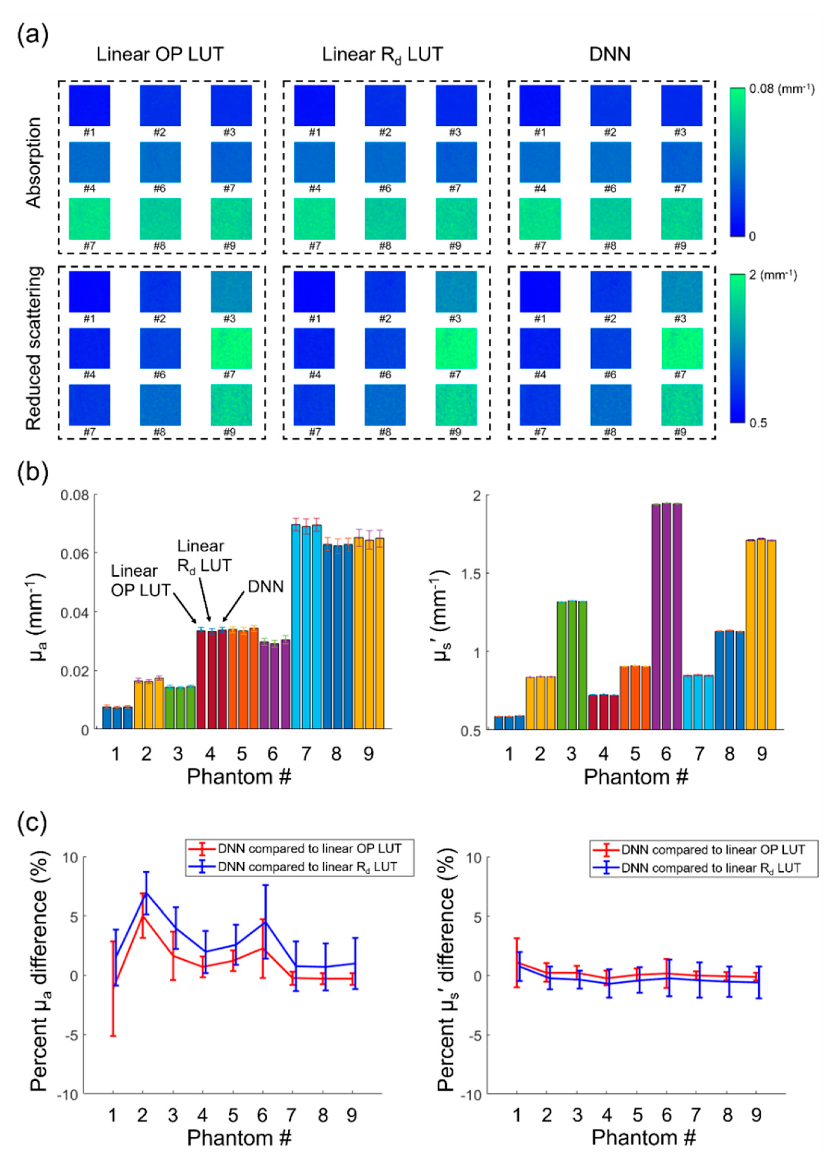
In addition to the speed and accuracy comparisons conducted with numerical simulation, the three inversion methods were also compared using experimental data measured from a set of nine homogeneous tissue-mimicking optical phantoms over a wide range of OPs. The optical phantom measurements were conducted using a commercial OxImager RS SFDI system (Modulated Imaging Inc., Irvine, CA, USA) at 659 nm. The image size was 696 × 520 pixels. A 100 × 100 pixels region in the center of the field-of-view was processed by the linear OP LUT, linear R_d LUT, and the DNN, and the results are shown in Figure 4. The figure shows that the three methods provide visually similar OP maps for all optical phantoms. Figure 4b shows the mean and standard deviation of the extracted optical property values. Figure 4c compares percent difference between the OPs values extracted by the DNN in reference to OPs extracted by the linear OP LUT and the linear R_d LUT. These data show that the three methods provide very similar OP values, with differences of less than 5.0% for µ_a and less than 1.1% for µ_s′ when comparing the DNN to the linear OP LUT.

The identified DNN was further demonstrated with experimental in vivo measurements on a cuff occlusion. The cuff was applied to the upper arm and the inner arm was measured with 0 and 0.1 mm⁻¹ spatial frequencies. The SFDI measurements were conducted using the commercial OxImager RS SFDI system at 659 nm and 851 nm. The image size was 696 × 520 pixels. The SFDI measurements were repeated approximately every 1.85 s for 150 timepoints with the commercial SFDI system. The measurement repetition rate here was chosen to be sufficient for monitoring the cuff occlusion process. After 1 min of baseline measurements, cuff pressure was rapidly increased to ~200 mmHg and lasted for 2 min. The measurement continued another 1.5 min after the cuff was released. The optical properties were calculated with the DNN, and the chromophore concentrations were calculated with Beer’s Law. The data processing and visualization were conducted in real-time, as shown in Supplementary Video S1 (Visualization 1).

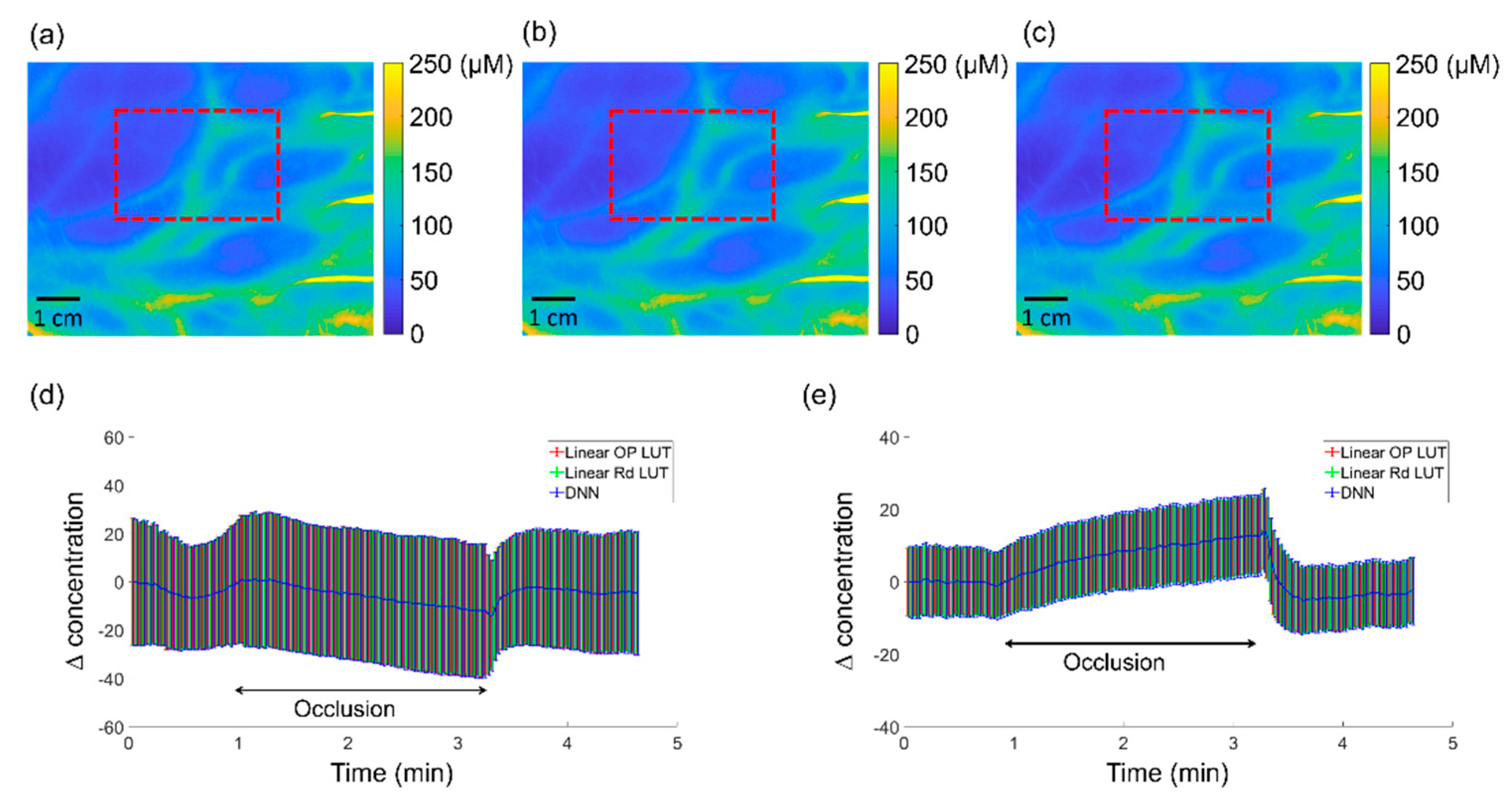
We compare the linear OP LUT, linear R_d LUT, and the DNN for chromophore concentration extraction on the cuff occlusion measurements. A large ROI on the tissue (200 × 300) was selected for processing by the three methods. This ROI is the same with the ROI used to calculated average chromophore changes in the supplementary video, and is indicated by the red dashed box in Figure 5a–c as well as in the video chromophore maps. With linear OP LUT, linear R_d LUT, and DNN, optical properties were first extracted, and then the HbO₂ and Hb concentrations were calculated using Beer’s Law.

The total hemoglobin maps estimated by the three methods for baseline cuff measurement are compared in Figure 5a–c. The mean and standard deviation results are plotted in Figure 5d,e below, as average changes in oxy-hemoglobin (HbO₂) and deoxy-hemoglobin (Hb), respectively. The data show that the mean and standard deviation results from the three methods overlap, indicating a good agreement. The relatively large standard deviation was due to the relatively large size of selected ROI (200 × 300 pixel).

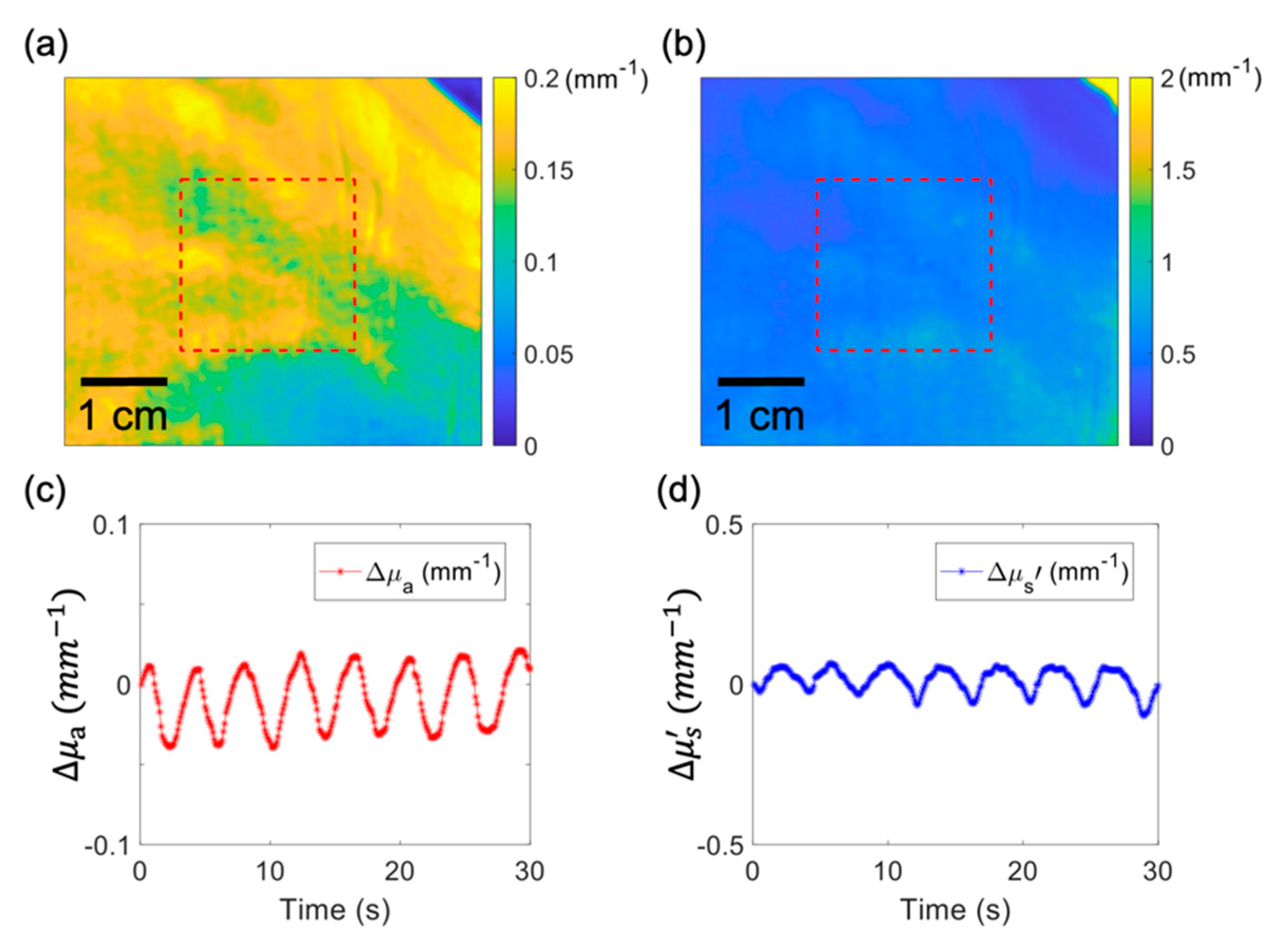
Furthermore, while video-rate acquisition has been reported in the literature, the corresponding real-time extraction of optical properties remains hindered by the slow speed of available inversion algorithms [11,12]. Here, we further demonstrate the fast inversion capability of the proposed DNN, by showing video-rate monitoring of optical properties for a subject’s free-moving hand. The measurement was conducted in accordance with an institutionally approved protocol. The subject’s hand was moving upward and downward freely and repeatedly in a quasi-periodic manner, while being measured at 685 nm with 0 and 0.1 mm⁻¹ spatial frequencies by a custom SFDI system. The measurements were conducted for 30 s with a repetition rate of 10 Hz. The data collection, processing and visualization were conducted in real-time, as shown in Supplementary Video S2 (Visualization 2). Figure 6 shows the last frame of the video. Figure 6a,b correspond to the extracted optical absorption and reduced scattering maps, respectively. Figure 6c,d correspond to the average changes in absorption and scattering of the tissue area shown by the red dashed box, respectively, indicating an apparent quasi-periodic change in optical properties induced by the movement of the subject’s hand. It is noted that the 10 Hz real-time monitoring of optical properties for a fast-moving object would not be feasible for previous OP inversion algorithms such as the linear OP LUT and linear R_d LUT methods due to limited inversion speed.

Finally, since GPUs have been widely used to speed up computations, we conducted OP inversion experiments using a typical GPU device and compared with a CPU under different pixel array sizes. The experiment settings are detailed in the Methods section. As shown in Figure 7, the blue and red curves represent average time costs for CPU and GPU devices, respectively. It shows that the GPU consistently required significantly less processing time compared with the CPU. In addition, the GPU has a particular advantage in terms of computation for large pixel arrays. For instance, with a 2000 × 2000 pixel array, the CPU required over 80 ms. In contrast, the GPU took less than 0.4 ms, which is over 200 times faster than the CPU.

4. Conclusions

In summary, this work explored the hyperparameter space, including the tradeoffs between speed and accuracy for different numbers of neural layers, the numbers of neurons in each layer and activation functions for DNNs for the SFDI inverse problem. An ultracompact, two-layer, deep learning framework was introduced and provided significantly faster computational speeds (30×–600×) with similar accuracy when compared to existing linear OP LUT and linear R_d LUT methods. While our previous deep learning work for optical property extraction requires 200 ms for an image size of 696 × 520 pixels [17], the DNN developed in this work is over 30× faster. In addition, the proposed DNN only needs minimal computing power to extract optical properties, and can potentially be implemented on the micro-processing unit (MPU). In contrast, the traditional methods such as the linear OP LUT with curve fitting require a significantly higher computing capability. With the ongoing development of deep learning technologies, one can envision integrating the DNN developed in this work with low-cost mobile devices, enabling the real-time wide-field mapping of optical properties, as well as the chromophores that can be used in a bedside or point-of-care setting.

5. Discussion

We note that since the output space for optical properties is continuous, and that the R_d-OP structure is essentially curved planes, the ReLU activation function was not suitable for the compact network structure in our study despite its popularity in pattern recognition and classification tasks [15]. This is because, by definition, ReLU is “semi-linear”. In other words, it is linear at (−∞, 0) and (0, +∞) regions, and its non-linearity comes from the near-zero region, which makes ReLU function not ideal to fit curve lines or planes under small network structures.

Since the optical property extraction is essentially conducted in a pixel-by-pixel manner, the speed of the calculation can be further enhanced by using specially designed hardware such as GPU or FPGA. For example, in Figure 7, we show the speed acceleration with GPU, and the results show that the GPU required less than 0.4 ms to process an 2000 × 2000 pixels image, making it over 200× faster than the CPU.

Going forward, there are several other directions that may further enhance the capabilities of the proposed DNN framework. The DNN can also be trained for other pairs of spatial frequencies, which may be useful for different tissue types and chromophores [29,30]. Additionally, the DNN demonstrated in this work can be further integrated with fast SFDI hardware to enable real-time, video-rate, or even kilohertz mapping of chromophore concentrations for pre-clinical, clinical, and industrial applications [31,32].