Article

Development of Singular Points in a Beam Passed Phase Screen Simulating Atmospheric Turbulence and Precision of Such a Screen Approximation by Zernike Polynomials

1
V.E. Zuev Institute of Atmospheric Optics, 634055 Tomsk, Russia
2
School of Energy and Power Engineering, National Research Tomsk Polytechnic University, 634050 Tomsk, Russia
*
Author to whom correspondence should be addressed.
Photonics 2022, 9(5), 285; https://doi.org/10.3390/photonics9050285
Submission received: 15 March 2022 / Revised: 18 April 2022 / Accepted: 19 April 2022 / Published: 21 April 2022
(This article belongs to the Special Issue Various Applications of Methods and Elements of Adaptive Optics)

Abstract

:
This article addresses two issues. Firstly, it was shown that if the initial phase of a Gaussian beam is specified by the sum of Zernike polynomials or by a screen simulating atmospheric turbulence, in the process of propagation, singular points appear in the wavefront of such a beam. With the use of numerical simulation, the dependence of the vortices number on the distortion characteristics and on the distance traveled by the beam was determined. The second problem analyzed in the article is the problem of a phase screen approximation by a series formed by Zernike polynomials. The carried out numerical experiments made it possible to determine the dependence of approximation accuracy on the screen parameters and on the number of polynomials entering the basis of approximation.

1. Introduction

The assessment of the effectiveness of correction for turbulent distortion of laser beams and the enhancement of correction quality are problems that have been studied for more than twenty years and are still actual at present [1,2,3,4,5]. Often, such problems are solved with the application of numerical methods, and in developed models, Zernike polynomials are often used to define the number of degrees of freedom of the active element of an adaptive system. Actually, a phase screen that defines the turbulent distortions of a beam is represented as a series of polynomials [4,5]. Therefore, it seems appropriate to carry out the numerical estimation of this expansion precision, to our knowledge, this problem has not yet been considered thoroughly.
Optical vortices (singular points or beam dislocations) are specific objects that appear sometimes in a wavefront of radiation [6]. Such objects are characterized by a small region of zero amplitude around the vortex and a cut in phase distribution. The cut ends in the center of a vortex. The development of optical vortices was observed in experiments with beams reflected from a rough surface [7,8]. At the same time, the authors of Refs [3,4] demonstrated in numerical [3] and laboratory experiments [4] that a beam propagating in a turbulent atmosphere acquires a complex form, and scintillations and intensity zeros appear in its amplitude distribution, so in the wavefront of such a beam, one can also expect the development of singular points. Beam control under such conditions presents considerable difficulties, for example, the negative influence of dislocations on the adaptive correction was theoretically demonstrated in Ref. [1].
The present article is a continuation of research in these areas. In the text, we discuss two problems. Firstly, in numerical experiments, we demonstrated that singular points appear in a wavefront of a Gaussian beam with an initial phase profile given by Zernike polynomials or by a screen simulating atmospheric turbulence, i.e., by a smooth function. To increase reliability, the number and coordinates of dislocations were found using three detection algorithms built on different principles [9,10,11,12]. Thus, the number of vortices in the wavefront as a function of turbulence intensity and the distance traveled by the beam was obtained.
The second problem, the solution of which is discussed in the article, is the problem of phase screen approximation. It is known, that to realize successfully the adaptive control of a laser beam in a turbulent atmosphere requires the precise reconstruction of a reference beam phase. Often this phase has a complex form and includes singular points, so the reconstruction of such distribution by an adaptive mirror with a continuous surface leads to errors in the process of beam control. It is expedient to analyze this problem by numerical methods, but to do so the whole mathematical and numerical model of an adaptive system is required. This model should include many rather complex blocks, so at the thirst stage, we just considered the precision of a phase screen approximation by Zernike polynomials. The obtained results and characteristics of the method are presented in the current paper.

2. Materials and Methods

The propagation of coherent laser radiation in a turbulent medium was considered on the base of the numerical simulation technique. The optical layout of the numerical experiment is shown in Figure 1. The beam had a Gaussian amplitude profile; phase modulation was realized in the plane of the emitting aperture by a surface formed as a sum of Zernike polynomials [13] or by a phase screen simulating atmospheric turbulence. The spectral density of the index of refraction fluctuations on this screen was given by the following equation [14]:
Φ n ( κ ) = 0.033 C n 2 ( κ L 2 + κ 2 ) 11 / 6 exp ( κ 2 / κ m 2 ) ,   κ L = 2 π / L 0 ,   κ m = 5.92 / l 0 .  
Equation (1) describes the von Karman spectrum of fluctuations, L0, l0 are the outer and inner scales of turbulence, Cn is the structure constant of atmospheric turbulence, related with Fried’s coherence length by the formula r 0 = 1.68 ( C n 2 k 2 L ) 3 / 5 , here k is the wave number, L is a path length. This formula demonstrates that r 0 depends on the intensity of the index of refraction fluctuations, wavelength, and on the distance passed by a beam.
From the screen to the plane of observation the beam propagated under conditions of free diffraction. Propagation was described by the wave equation [15]:
2 i k ( E z + 1 v g r E t ) = Δ E ,
and the fast Fourier transform was employed to solve it [16]. In Equation (2), x and y are coordinates in the plane normal to the direction of propagation; z is a coordinate along this direction; Δ = 2 / x 2 +   2 / y 2 is the Laplace operator; vgr is the group velocity of the beam. The coordinates x and y, and parameter r0 were normalized to the beam initial radius a0, and coordinate z to the diffraction length z d = k a 0 2 . All computer applications used in investigations of singular beam propagation were developed by the authors of the paper with Visual C++ language [17].
The following set of parameters was used to characterize the optical field in the plane of observation: Power-in-the-bucket (PIB).
J ( t ) = 1 P 0 ρ ( x , y ) I ( x , y , t ) d x d y .
This parameter is proportional to the beam power incident in an aperture of radius St. In Equation (3) P0 is the total power of the beam and
ρ ( x , y ) = exp [ ( x 2 + y 2 ) / S t 2 ]
is an aperture function.
The shift of the beam gravity center along axis x:
X c = 1 P 0 a 0 x I ( x , y , t ) d x d y ,
and y:
Y c = 1 P 0 a 0 y I ( x , y , t ) d x d y .
The effective radius of the beam
R E f f = { 1 P 0 a 0 ( r r c ) 2 I ( x , y , t ) d x d y } 1 / 2 .
To obtain complete information concerning beam distortions, in addition to the above-described functions, we also registered the quantity and coordinates of optical vortices developed in the wavefront. The detailed description of the algorithms constructed to localized singular points of the wavefront was given in Ref. [9]. Algorithms were built with the use of the following special features of vortex radiation:
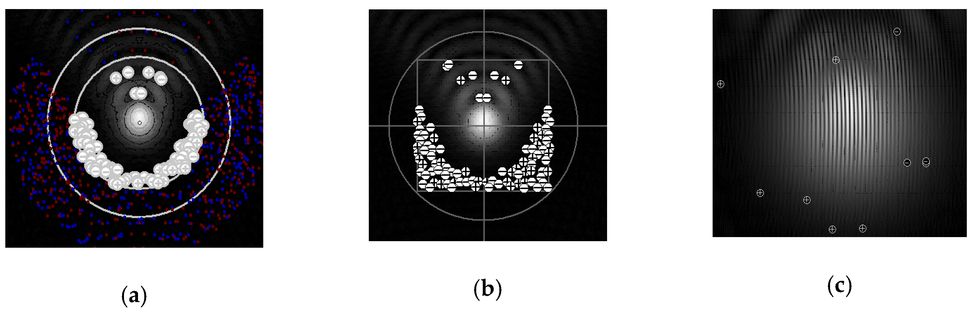
  • Branch cuts are present in an interference pattern of vortex radiation. On this property, the first algorithm was developed.
  • Circulation Γ(α) of wavefront gradients
    Γ ( α ) = P α ( r , z ) d r
    is equal to ± 2 π n if an optical vortex falls in an integration contour. The second algorithm was based on this property. Here n is a vortex topological charge and P is the perimeter of the integration contour.
  • A vortex is a point of intersections of isolines. Isolines should be drawn in distributions of real and imaginary parts of beam complex amplitude, magnitudes of corresponding functions were equal to zero along the line. On this property, the third algorithm was developed.
According to the assessments presented in Ref. [9], the highest precision of registration was achieved with algorithms 2 and 3. Computer processing of interference patterns (algorithm No. 1) does not provide high resolution, so only a small number of vortices can be localized with the application of this method.

3. Obtained Results

In the present paragraph, the results characterizing the development of singular points in a wavefront of radiation are presented. The phase profile of radiation has been formed as a sum of Zernike polynomials [14], or specified by a phase screen, simulating atmospheric turbulence. Furthermore we illustrated the quality of approximation of such a screen.
Changes in Gaussian beam amplitude are shown in Figure 2, Figure 3, Figure 4 and Figure 5, while its initial phase was formed by a single polynomial. In the pictures, we can see the phase distribution of radiation (Figure 2a), cross-sections of this distribution (Figure 2b), and amplitude distribution of a beam passed a distance of 0.1 diffraction length (Figure 2c).
In the pictures, we can see the phase distribution of radiation (Figure 2a, Figure 3a, Figure 4a and Figure 5a), cross-sections of this distribution (Figure 2b, Figure 3b, Figure 4b and Figure 5b), and amplitude distribution of a beam passed a distance of 0.1 diffraction length (Figure 2c, Figure 3c, Figure 4c and Figure 5c).
Usually, an approximation of a screen simulating atmospheric turbulence is performed by the sum of polynomials [14], so it is feasible to consider influence induced not only by discrete components but also by the total sum of components. Corresponding examples are shown in Figure 6 and Figure 7; in Figure 6, summation was realized from the first to sixth (trefoil) polynomials and in Figure 7 to the seventh (coma). All coefficients were the same and equal to one.
Registered distributions of singular points are presented in Figure 8 and Figure 9, corresponding phase profiles were set by such polynomials as coma (Figure 8) and trefoil (Figure 9). To improve the reliability of results dislocations were localized by three algorithms built on different principles.
The dependence of dislocation quantity on polynomial number is shown in Figure 10. The radius of a region where detection was performed changed in the range from 1 to 1.4 initial radii of a beam.
The number of the found vortices as a function of the distance traveled by a beam is presented in Figure 11 and Figure 12. The initial phase was formed by such polynomials as coma and trefoil (Figure 11) or set by a phase screen representing atmospheric turbulence (Equation (1)).
The results presented above demonstrate that the development of optical vortices is possible in a beam with an initially smooth phase profile. Let us now consider the possibility of such a profile approximation by Zernike polynomials. In the first of the two problems, the phase was represented by the sum of polynomials and approximated by the sum of polynomials, in the second, the phase was set by a turbulent screen and approximated by polynomials. In the process of approximation calculation of polynomial coefficients was realized with the least-mean-square method [15].
The first problem we divided into three variants:
The numbers of polynomials entering the basis of approximation are larger than that in the phase screen (Table 1; 12 and 9 polynomials correspondingly).
The screen and approximation basis include the same number of functions (Table 2, Table 3 and Table 4).
The number of polynomials in the basis is lesser than in the phase screen (Table 5).
The initial phase profile and the surface obtained as a result of approximation were formed by the same functions, so to assess the precision of calculations we can compare coefficients of the members entering the sum and deviation of one surface from another. Corresponding parameters (coefficients CZN, here, N is a polynomial number) were put in Table 1, Table 2, Table 3, Table 4 and Table 5. The difference between the two surfaces was calculated according to the formula
ε Ph = i , j M ( A i j B i j ) 2 / i , j M ( A i j ) 2
here, Aij is the value of the given function in node i, j; Bij is the value of the function obtained as a result of approximation; M × M are dimensions of the computational grid.
To increase the consistency of the solution, we compared the parameters of two beams with Gaussian amplitude distributions. The phase of the first was set by the screen formed by the sum of polynomials (Figure 1), while for the phase of the second, the surface taken obtained was in the approximation procedure. Both beams passed the same distance, after that their parameters were calculated and compared. Calculation of the following parameters was performed: power-in-the-bucket J (Equation (3)), shifts XC and YC of beam gravity center along OX and OY axes (Equations (4) and (5)), the effective radius of the beam REff (Equation (6)). Furthermore, we calculated the difference between amplitude distributions. To do so, Equation (8) was used, but instead of phase profiles, we substituted into the formula corresponding amplitude distributions.
Results obtained in the first variant are presented in Table 1. The basis of approximation was formed by 12 polynomials, and 9 polynomials were included in the phase screen.
In the second variant, an equal number of polynomials were included in the basis and screen. In Table 2, the date is presented for the screen formed by 9, and in Table 3 and Table 4 by 12 polynomials.
The third variant is illustrated by the results given in Table 5 and in Figure 13.
The next problem is the approximation of the phase screen simulating turbulent fluctuations of the index of refraction. As in the previous example, propagation was analyzed by two beams with Gaussian amplitude distributions. The phase of the first was set by the phase screen, while the phase of the second was obtained as a result of approximation. Parameters of beams calculated in the plane of observations were presented in Table 6, Table 7 and Table 8; in Figure 14, Figure 15 and Figure 16, we can see amplitude distributions and phase profiles of the beams.
Calculations were performed with different intensities of atmospheric distortions and with the use of different calculation grids. In all numeric experiments, the inner scale of turbulence was larger than the diameter of the beam. Even under such conditions, the quality of the screen approximation was not high, but with a smaller inner scale, the obtained results were completely unsatisfying.

4. Discussion

4.1. Scintillations of Amplitude and Emergence of Singular Points in the Wavefront of a Beam with a Phase Set by Zernike Polynomials

The first block of results included in paragraph 3 of the current paper illustrates the fact that a singular wavefront can be obtained if the initial phase profile of a beam is set to be Zernike polynomials. To prove this fact, the beam with a given phase passed some distance in a non-aberrating medium, its amplitude and phase profiles were calculated in the plane of observations (the optical layout of the corresponding numerical experiment is shown in Figure 1), and singular points were registered by three different algorithms.
Figure 2, Figure 3, Figure 4, Figure 5, Figure 6 and Figure 7 show that points of zero intensity appear in such a beam, the localization of optical vortices is illustrated in Figure 8 and Figure 9. If a phase profile is formed by a sum of polynomials with equal coefficients, amplitude distribution is influenced mainly by the last polynomial entering the sum. This can be seen from the comparison of Figure 3 and Figure 6. In the first case, the phase was set by trefoil, and in the second by the sum including polynomials from the first to trefoil. All polynomial coefficients were the same and equal to one. In both variants (Figure 3c and Figure 6c) amplitude distributions have similar forms. The same conclusions can be drawn if we compare Figure 4c and Figure 7c, corresponding amplitude profiles were obtained by setting the phase with coma and by sum including polynomials from the first to coma.
In the observation plane, we also survey the appearance of singular points in the wavefront of the beam. The application of two registration algorithms gives approximately the same results, i.e., close numbers of vortices and similar forms of their distribution (Figure 8a,b and Figure 9a,b). A much smaller number of singular points were localized by the interferometric algorithm (Figure 8c and Figure 9c) which can be explained by the low resolution by the applied technique. Nevertheless, in all situations the vortices were detected, which proves the development of singular points in a beam with an initially smooth phase profile.
Data illustrating the dependence of dislocation number on the size of the registration region, number of polynomials setting the phase profile, and the beam propagation distance are presented in Figure 10, Figure 11 and Figure 12. As is shown in Figure 10, vortices do not appear if the phase is prescribed with the use of the first five polynomials. The singular points started to appear from the polynomial number six and higher. Comparing the form of curves in Figure 10, we can deduce that number of vortices increases with the increase in the region radius where we look for singular points.
The dependence of dislocation quantity on the distance passed by the beam is shown in Figure 11. The phase was set by polynomials. Characteristic features of all curves are oscillations and general decreases.
Approximately the same traits we observe if the phase is given by the screen simulating atmospheric turbulence (Figure 12). As in the previous graph, the curves oscillate, pass maximums, and go to zero.

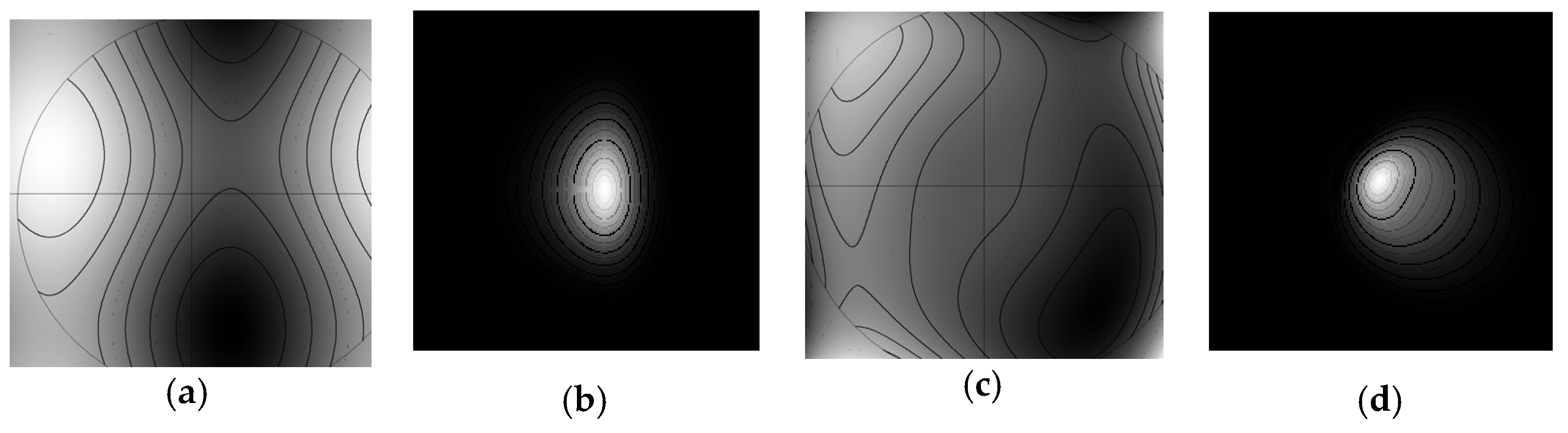
4.2. Approximation of the Phase Screen Formed by Zernike Polynomials

In the previous part, we demonstrated that optical vortices appear in a wavefront if a beam passes the phase screen formed by Zernike polynomials. Let us consider how precisely we can approximate such a screen by a series of polynomials. Of course, the actual problem is the approximation of a screen simulating turbulent distortions, but to assess the precision of the method we simplified the project. The obtained results are presented in Table 1, Table 2, Table 3, Table 4 and Table 5. The accuracy of the method was characterized by the deviation of the given polynomial coefficients from coefficients calculated by the least-mean-square method [18]. We also compared the parameters of two beams, the phase of the first was set by the screen, and the phase of the second was obtained as the result of approximation. Both beams passed the same distance.
If the phase was set as a sum of nine polynomials and the basis of approximation was larger (Table 1, 12 polynomials in the basis) or the same (Table 2, 9 polynomials in the basis), high precision can be achieved even with small-scale (256 × 256 nodes) computational grids. In this case, values of all calculated coefficients coincided with values of given coefficients. Astigmatism is an exception, but in this case, the main influence on amplitude exerts not the magnitude but the difference between coefficients of two astigmatisms, and this difference was calculated correctly.
The precision of phase reconstruction decreases with the increase in polynomial number in the sum forming the screen (Table 3 and Table 4). Unsatisfying results were obtained with the application of small-dimension grids (Table 3). A large difference was observed between values of coefficients (columns 1 and 2 of Table 3), as well as between parameters of the two beams (columns 8–13).
The accuracy of approximation can be increased with an increase in the grid dimensions (Table 4, the grid with 2048 × 2048 nodes), but notwithstanding the small difference between coefficients registered in this case (Table 4, columns 1–7) and coincidence of such integral parameters as effective radius and shift of gravity center along coordinate axes (columns 11–13), the phase of two beams differs by 22% and amplitude by 14% (columns 9 and 10).
Least-mean-square techniques also give incorrect results when the number of polynomials in the basis of approximation is smaller than in the phase screen. Corresponding data are given in Table 5 and in Figure 13. To reduce the influence of the last polynomial in the sequence forming the screen we decreased the magnitude of its coefficient from 1.0 to 0.2. However, even such lessening of its influence did not cause a coincidence in the results, the calculated parameters of the two beams were dissimilar (Table 5, columns 8–13), and the difference between their amplitude profiles can be seen by the naked eye (Figure 13).

4.3. Approximation of a Phase Screen Simulating Atmospheric Distortions

In this problem, the same model was used as in the previous part, i.e., the phase of the beam was set by a screen, then this screen is approximated by a sum of polynomials, and obtained distribution was employed as an initial phase profile of a beam with Gaussian amplitude profile. After propagation on some distance parameters, two beams were compared. Specifically, we can compare the difference in the initial phase of two beams, their amplitude distributions in the plane of observations, PIBs, shifts of gravitation centers, and so on. Corresponding parameters were put in Table 6, Table 7 and Table 8 and presented in Figure 14, Figure 15 and Figure 16.
Comparing images in Figure 14a,c we can see that the phase profiles of two beams are not unlike, though the positions of extremums (the brightest and darkest regions) in two pictures are slightly shifted. As a result, in the plane of observations, we register the same magnitudes of PIBs (Table 6, column 3) and the same shifts of gravity centers (columns 4 and 5). The largest difference is observed in the magnitudes of effective radii (column 6–8), consequently, amplitude distributions of two beams do not also coincide (Figure 14b,c).
With the increase in turbulent intensity characterized by Fried’s coherence length, the main features of the problem remain the same, the phase profiles of the two beams are similar, the effective radii and amplitude distributions are different (Table 7 and Figure 15).
The increase in the solution accuracy cannot be achieved by increasing the grid dimensions up to 2048 × 2048 nodes (Figure 16 and Table 8). In this case, the difference between amplitude distributions is approximately 68% (Table 8, column 2), effective radii along axes OX and OY of the second beam were calculated erratically (columns 6–8 of the Table), and some errors appeared in the calculation of gravity center shifts (column 5). In general, even with the large inner scale, we could not obtain the exact approximation of the phase screen simulating the influence of atmospheric turbulence. If the inner scale decreases, the quality of approximation decreases even further.

5. Conclusions

The data presented in the paper allow one to draw the following conclusions:
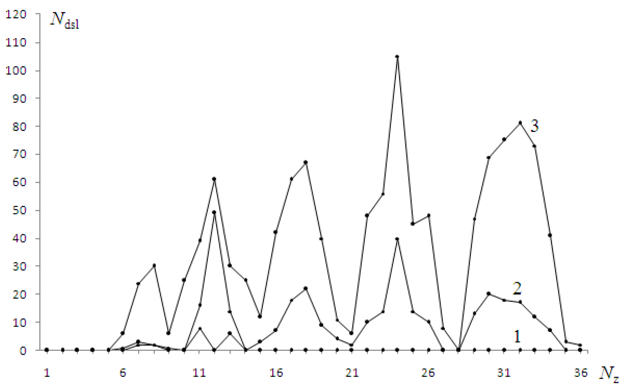
  • If a phase profile of a beam with Gaussian distribution of amplitude is set by high Zernike polynomials, scintillations of intensity and optical vortices appear in such a beam as a result of propagation. With the increase in propagation distance, the number of vortices changes and decreases.
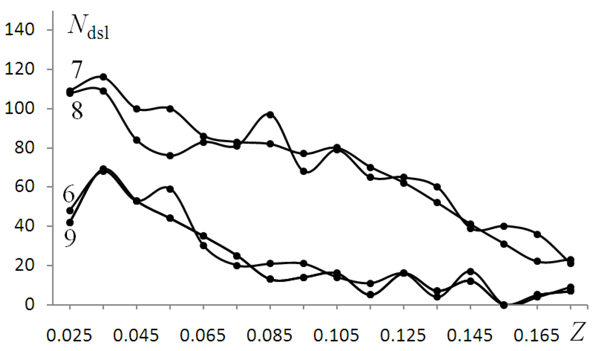
  • Singular points of the wavefront also appear if the phase is set by a screen simulating atmospheric turbulence. Dependence on the path length is approximately the same as in the previous case: corresponding curves oscillate, reach maximums, and go to zero.
In the problem of approximation of the phase screen formed by Zernike polynomials, (approximation was also performed by the polynomials) we established that:
  • If a phase screen is formed by 9 polynomials and the basis of approximation is formed by the same or greater number of polynomials high precision can be achieved even with computational grids of small dimensions (256 × 256 nodes).
  • The quality of approximation decreases if the number of polynomials forming the screen increases (we have considered an increase in numbers up to 12). Absolutely unsatisfying results were observed on grids with small dimensions.
  • The precision of the solution can be increased with the increase in the grid dimensions, but even on 2048 × 2048 grid the difference between given and calculated phase profiles (Equation (7)) is about 22%.
The approximation of a phase screen simulating turbulence of medium intensity showed that errors of phase restoration depend on Fried’s coherence length. In all considered cases, these errors changed from 22% to 24%. Much larger (from 30% to 68%) were differences between amplitude profiles of beams.

Author Contributions

Conceptualization, software development, and original draft preparation were done by F.K. Reviewing anf editing by N.M. Calculations and analyzes of results by I.V. All authors have read and agreed to the published version of the manuscript.

Funding

Parts 2 and 3 of this research were funded by Russian Science Foundation (project No. 20-19-00597). Part 4 was funded in the framework of the State program formulated for the Institute of atmospheric optics SB RAS, Tomsk, Russia.

Institutional Review Board Statement

Npt applicable.

Informed Consent Statement

Not applicable.

Data Availability Statement

Not applicable.

Conflicts of Interest

The authors declare no conflict of interest.

References

  1. Fried, D.L. Branch point problem in adaptive optics. J. Opt. Soc. Am. A 1998, 15, 2759–2767. [Google Scholar] [CrossRef]
  2. Vorontsov, M.A.; Kolosov, V.V.; Kohnle, A. Adaptive laser beam projection on an extended target: Phase- and field-conjugate precompensation. J. Opt. Soc. Am. A 2007, 24, 1975–1993. [Google Scholar] [CrossRef] [PubMed]
  3. Konyaev, P.A.; Lukin, V.P. Computational algorithms for simulations in atmospheric optics. Appl. Opt. 2016, 55, B107–B112. [Google Scholar] [CrossRef] [PubMed]
  4. Lachinova, S.L.; Vorontsov, M.A. Laser beam projection with adaptive array of fiber collimators. II. Analysis of atmospheric compensation efficiency. J. Opt. Soc. Am. A 2008, 25, 1960–1973. [Google Scholar] [CrossRef] [PubMed]
  5. Noll, R.J. Zernike polynomials and atmospheric turbulence. J. Opt. Soc. Am. 1976, 66, 207–211. [Google Scholar] [CrossRef]
  6. Grier, D.G. A revolution in optical manipulation. Nature 2003, 424, 810–816. [Google Scholar] [CrossRef] [PubMed]
  7. Li, X.; Tai, Y.; Zhang, L.; Li, H.; Li, L. Characterization of dynamic random process using optical vortex metrology. Appl. Phys. B 2014, 116, 901–909. [Google Scholar] [CrossRef]
  8. Wang, W.; Qiao, Y.; Ishijima, R.; Yokozeki, T.; Honda, D.; Matsuda, A.; Hanson, S.G.; Takeda, M. Constellation of phase singularitie in a specklelike pattern for optical vortex metrology applied to biological kinematic analysis. Opt. Express 2008, 16, 13908–13917. [Google Scholar] [CrossRef] [PubMed]
  9. Kanev, F.; Aksenov, V.P.; Veretekhin, I.D.; Makenova, N.A. Methods of optical vortex registration. In Proceedings of the 25th International Symposium on Atmospheric and Ocean Optics: Atmospheric Physics, Novosibirsk, Russia, 1–5 July 2019. [Google Scholar]
  10. Patorski, K.; Pokorski, K. Examination of singular scalar light fields using wavelet processing of fork fringes. Appl. Opt. 2011, 50, 773–781. [Google Scholar] [CrossRef] [PubMed]
  11. Angelsky, O.V.; Maksimyak, A.P.; Maksimyak, P.P.; Hanson, S.G. Spatial Behaviour of Singularities in Fractal-and Gaussian Speckle Fields. Open Opt. J. 2009, 3, 29–43. [Google Scholar] [CrossRef] [Green Version]
  12. Nye, J.F. Natural Focusing and Fine Structure of Light: Caustics and Wave Dislocations; Institute of Physics Publishing: Bristol, PA, USA; Philadelphia, PA, USA, 1999; 328p. [Google Scholar]
  13. Svechnikov, M.V.; Chkhalo, N.I.; Toropov, M.N.; Salashchenko, N.N. Resolving capacity of the circular Zernike polynomials. Opt. Express 2015, 23, 14677–14693. [Google Scholar] [CrossRef] [PubMed]
  14. Chaudhary, V.; Abhilash, A. Literature review: Mitigation of atmospheric turbulence on long distance imaging system with various methods. Int. J. Sci. Res. 2012, 3, 2227–2231. [Google Scholar]
  15. Andrews, L.C.; Phillips, R.L. Laser Beam Propagation through Random Media, 2nd ed.; SPIE Press Book: Bellingham, WA, USA, 2005; 808p. [Google Scholar]
  16. Heideman, M.T.; Johnson, D.H.; Burrus, C.S. Gauss and the history of the Fast Fourier Transform. IEEE ASSP Mag. 1984, 1, 14–21. [Google Scholar] [CrossRef] [Green Version]
  17. Lippman, S.B.; Lajoie, J.; Moo, B.E. C++ Primer, 5th ed.; Addison-Wesley: Boston, MA, USA, 2013; 938p. [Google Scholar]
  18. Gui, G.; Adachi, F. Improved least mean square algorithm with application to adaptive sparse channel estimation. EURASIP J. Wirel. Commun. Netw. 2013, 2013, 204. [Google Scholar] [CrossRef] [Green Version]
Figure 1. Layout of numerical experiments.
Photonics 09 00285 g001
Figure 2. Phase specification by polynomial No. 5 (third-order astigmatism). Phase surface (a) and corresponding amplitude distribution of the beam passed path of 0.1 diffraction length (c) are shown by grayscale images. Cross-sections of the phase surface are presented in picture (b). Cross-section 1 was cut through the center of the beam, cross-section 2 corresponds to the cut shifted on the beam radius from the center in a positive direction of the y-axis, and number 3—to the cut shifted in a negative direction.
Photonics 09 00285 g002
Figure 3. The same as in Figure 2, but the phase was specified by polynomial No. 9 (trefoil). Phase surface (a), cross-sections of phase surface (b) and corresponding amplitude distribution (c) are shown. Three cross-sections coincide (b).
Photonics 09 00285 g003
Figure 4. The same as in Figure 2, the phase was specified by polynomial No. 7 (coma). Phase surface (a), cross-sections of phase surface (b) and corresponding amplitude distribution (c) are shown. Three cross-sections coincide (b).
Photonics 09 00285 g004
Figure 5. The same as in Figure 2, the phase was specified by polynomial No. 20. Phase surface (a), cross-sections of phase surface (b) and corresponding amplitude distribution (c) are shown.
Photonics 09 00285 g005
Figure 6. The same as in Figure 2, the phase was specified by the sum of polynomials from 1 to 6. Phase surface (a), cross-sections of phase surface (b) and corresponding amplitude distribution (c) are shown.
Photonics 09 00285 g006
Figure 7. The same as in Figure 2, the phase was specified by the sum of polynomials from 1 to 7. Phase surface (a), cross-sections of phase surface (b) and corresponding amplitude distribution (c) are shown.
Photonics 09 00285 g007
Figure 8. Distributions of singular points in a beam with a phase profile set by polynomial No. 8 (coma). The dislocations are shown by circles with «+» or «−» signs. To register optical vortices three algorithms were used. Firstly, vortices were localized by processing distribution of wavefront gradients (a); secondly, as a point of intersection of isolines (b); and with application of interferometric algorithm (c). The number of the found singular points Ndsl = 98 (a), Ndsl = 92 (b) и Ndsl = 10 (c). The normalized path length was equal to 0.1.
Photonics 09 00285 g008
Figure 9. The same as in Figure 8, but the phase was specified by polynomial No. 9 (trefoil). Ndsl = 58 (a), Ndsl = 43 (b) и Ndsl = 7 (c).
Photonics 09 00285 g009
Figure 10. Number of singular points (Ndsl) in a beam wavefront with a phase specified by different polynomials (Nz). Registration was carried out in a region with a radius equal to the initial radius of a beam (curve 1), to two initial radii (2), to three initial radii (3). Z = 0.1.
Photonics 09 00285 g010
Figure 11. Dependence of dislocation number on distance Z passed by the beam. Calculation was performed for a beam with phase specified by two comas (polynomial numbers and number of curves are 7 and 8) and by trefoils (polynomials and curves are 6 and 9). The radius of registration region is 1.4 of the initial radius of the beam.
Photonics 09 00285 g011
Figure 12. Dependence of dislocation number on distance Z passed by the beam. Calculation was performed for several realizations of random phase screens, numbers of which are printed near curves.
Photonics 09 00285 g012
Figure 13. A beam amplitude registered at the distance of 0.1 diffraction length (a) and its initial phase (b) represented as the sum of the first nine polynomials. All polynomial coefficients except No. 9 were equal to one; the ninth coefficient was equal to 0.2. Amplitude (c) and phase (d) profiles obtained as a result of approximation with the use of eight polynomials.
Photonics 09 00285 g013
Figure 14. Precision of phase screen approximation. Phase distribution specified by the screen simulating atmospheric turbulence (a), amplitude distribution of a beam with initial phase profile specified by this screen (b), surface obtained as a result of approximation (c), amplitude of a beam (d) with initial phase presented in Figure (c). Dimensions of computation grid are 1024 × 1024, r0 = 0.2.
Photonics 09 00285 g014
Figure 15. Increase in turbulence intensity (r0 = 0.1). Other parameters of numeric experiment are the same as in Figure 14. Phase distribution specified by the screen simulating atmospheric turbulence (a), amplitude distribution of a beam with initial phase profile specified by this screen (b), surface obtained as a result of approximation (c), amplitude of a beam (d) with initial phase presented in Figure (c).
Photonics 09 00285 g015
Figure 16. Results obtained with computational grid of larger (2048 × 2048 nodes) dimensions. Other parameters are the same as in the previous example (Figure 15, Table 6). Phase distribution specified by the screen simulating atmospheric turbulence (a), amplitude distribution of a beam with initial phase profile specified by this screen (b), surface obtained as a result of approximation (c), amplitude of a beam (d) with initial phase presented in Figure (c).
Photonics 09 00285 g016
Table 1. The screen was set by 9 polynomials and approximated by 12 polynomials. Dimensions of computational grid are 256 × 256 nodes.
ParametersCZ1CZ2CZ3CZ4CZ5CZ9JεPhεAREffXcYc
Number of the column 12345678910111213
Values of parameters corresponding to the given phase1.001.001.501.000.501.000.510.000.001.860.36−0.36
Values
obtained as a result of approximation
1.001.00−6.111.00−7.101.000.510.000.001.860.36−0.36
Table 2. The screen was set by 9 polynomials and approximated by 9 polynomials. Dimensions of computational grid are 256 × 256 nodes.
ParametersCZ1CZ2CZ3CZ4CZ5CZ9JεPhεAREffXcYc
Number of the column12345678910111213
Values of parameters corresponding to the given phase1.001.001.501.000.501.000.510.000.001.860.36−0.36
Values
obtained as a result of approximation
1.001.00−6.111.00−7.111.000.510.000.001.860.36−0.36
Table 3. The screen was set by 12 polynomials and approximated by 12 polynomials. Dimensions of computational grid are 256 × 256 nodes.
ParametersCZ1CZ2CZ3CZ4CZ5CZ12JεPhεAREffXcYc
Number of the column12345678910111213
Values of parameters corresponding to the given phase1.001.001.501.000.501.000.520.000.002.350.07−0.07
Values
obtained as a result of approximation
19.27−3.9−1452.11.00−1413.11.000.184.100.693.210.440.39
Table 4. The screen was set by 12 polynomials and approximated by 12 polynomials. Dimensions of computational grid are 2048 × 2048 nodes.
ParametersCZ1CZ2CZ3CZ4CZ5CZ12JεPhεAREffXcYc
Number of the column12345678910111213
Values of parameters corresponding to the given phase1.001.001.501.000.501.000.530.000.002.250.06−0.07
Values
obtained as a result of approximation
0.950.77952.221.00960.121.000.540.220.142.240.06−0.07
Table 5. The screen was set by 9 polynomials and approximated by 8 polynomials. Polynomial coefficient No. 9 was reduced to 0.2. Dimensions of computational grid are 1024 × 1024 nodes.
ParametersCZ1CZ2CZ3CZ4CZ5CZ8JεPhεAREffXcYc
Number of the column12345678910111213
Values of parameters corresponding to the given phase1.001.001.001.001.001.000.520.000.002.350.56−0.41
Values
obtained as a result of approximation
46.611.0017.831.0017.831.000.138.190.693.471.95−0.36
Table 6. Characteristics of the beam in the plane of observations. Parameters of numeric experiment were the same as in the previous example (Figure 14).
ParametersεPhεAmpJShXShYREffXREffYREff
Number of the column12345678
Values of parameters corresponding to the given phase000.9880.0430.0190.0530.0840.099
Values
obtained as a result of approximation
0.2080.2910.9860.0430.0190.0770.0750.107
Table 7. Characteristics of the beam in the plane of observations calculated with increased turbulence intensity. Parameters of numeric experiment were the same as in the previous example (Figure 15).
ParametersεPhεAmpJShXShYREffXREffYREff
Number of the column12345678
Values of parameters corresponding to the given phase000.9830.0760.0350.0380.0920.100
Values
obtained as a result of approximation
0.2080.5440.9800.0760.0350.0850.0780.114
Table 8. Characteristics of the beam in the plane of observations. Parameters of numeric experiment were the same as in the previous example (Figure 16).
ParametersεPhεAmpJShXShYREffXREffYREff
Number of the column12345678
Values of parameters corresponding to000.9650.076−0.1490.0390.0810.090
Values
obtained as a result of approximation
0.2440.6750.9550.076−0.1350.0930.1220.153
Publisher’s Note: MDPI stays neutral with regard to jurisdictional claims in published maps and institutional affiliations.

