Article

Low-Complexity Chromatic Dispersion Equalization FIR Digital Filter for Coherent Receiver

College of Intelligence Science and Technology, National University of Defense Technology, Changsha 410073, China
*
Author to whom correspondence should be addressed.
Photonics 2022, 9(4), 263; https://doi.org/10.3390/photonics9040263
Submission received: 9 November 2021 / Revised: 12 March 2022 / Accepted: 16 March 2022 / Published: 15 April 2022

Abstract

:
This paper proposes a novel and efficient low-complexity chromatic dispersion equalizer (CDE) based on finite impulse response (FIR) filter architecture for polarization-multiplexed coherent optical communication systems. The FIR filter coefficients are optimized by weights to reduce the energy leakage caused by the truncation effect, and then quantization is used uniformly to reduce the number of real number additions and real number multiplications by utilizing the diversity of the quantized coefficients. Using Optisystem 15 to build a coherent optical communication system for simulation and experimental demonstration, the results show that after the filter coefficients are optimized by weights. Compared with the time-domain chromatic dispersion equalizer (TD-CDE), the proposed design has a lower bit error rate (BER) and better equalization effect. When the transmission distance is 4000 km and the system quantization stages M = 16, the multiplication operation and addition operations reduce computing resources by 99% and 43%, and the BER only increases by 5%. Compared with frequency-domain chromatic dispersion equalizer (FD-CDE), widely used in long-distance communication, the multiplication operation reduces computing resources by 30%. The proposed method provides a new idea for high-performance CDE in long-distance coherent optical communication systems.

1. Introduction

In wired communication systems, the traditional coaxial cable communication is limited by the transmission distance and gradually replaced by optical fiber communication with strong anti-electromagnetic interference and long transmission distance. For optical signals with different frequency components or different model components, the signal pulses are broadened due to different group velocities, which causes signal distortion after being transmitted through the optical fiber. This physical phenomenon is called chromatic dispersion (CD) [1]. As the CD accumulates, the front and rear optical pulses overlap, causing inter-symbol interference (ISI) and increasing the bit error rate (BER). Therefore, the CD is one factor that restricts the development of optical fiber transmission systems to ultra-high-speed, ultra-large capacity, and ultra-long distance.
Although dispersion compensation fibers (DCF) or dispersion-compensating modules (DCM) allow CDE in the optical domain, this increases the complexity and cost of technical implementation. The digital coherent receivers perform CDE in the electrical domain, restore the broadening and distortion of the pulse signal, achieve dynamic compensation, and have been widely used in high-speed coherent optical communication systems [2,3,4,5] The digital filters used for CDE involving the time-domain chromatic dispersion equalizer (TD-CDE) filter and frequency-domain chromatic dispersion equalizer (FD-CDE) filter [6,7,8]. The CDE module occupies a large power consumption in the DSP, and a large number of calculation units also limit the development of the coherent receiver to a compact size [9] Therefore, the CDE module should reduce the algorithm complexity and hardware implementation conditions to improve the efficiency of coherent receivers [10,11]. Although the FD-CDE method is considered the best choice for commercial coherent receivers, due to the need for time-frequency conversion of the input sequence, this may cause time aliasing and weak interaction with other TD modules limiting the reduction of energy consumption [12]. The whole process of TD-CDE is carried out in TD, which avoids the problems of FFT block size and time aliasing. So in this paper, we mainly discuss TD-CDE and its optimization methods.
The traditional truncation process can be regarded as a rectangular window function to truncate the infinite and non-causal TD impulse response function. The ratio of the main lobe energy of the window function to the total energy determines the filtering performance after truncation to a certain extent. The spectrum side lobe of the rectangular window is high, and high-frequency interference is easily brought into the window transformation [13]. To further improve the performance of the window function, a series of classic window functions such as the Hanning window, Blackman–Harris window, and Rife–Vincent window is proposed [13]. However, these window functions still cannot meet the requirements of the narrow main lobe, small side lobe, and fast attenuation simultaneously. Jia proposed the use of rectangular shape pulse self-convolution to design a triangular-shaped pulse [14]. On this basis, Hanning convolution windows, triangular self-convolution windows, and hybrid convolution windows composed of rectangular windows and cosine windows have been successively proposed [15,16]. Although the method mentioned above has a certain improvement effect, application of the TD-CDE still needs to be verified. The number of taps in the TD-CDE filter is positively correlated with the accumulative CD in the channel. For ultra-high-speed long-distance coherent optical communication systems, achieving CDE requires lots of TD-CDE filter taps, and the amount of calculation is very large.
In this paper, we propose a lower-complexity TD-CDE filter structure, which is shown in the next Section. The main contributions of this paper are in two aspects. The first aspect is the use of a more superior Nuttall second-order self-convolution window instead of a rectangular window, effectively reducing the impact of energy leakage on filter performance. In order to reduce the computational complexity during convolutional operations, to be suitable for the long-distance coherent optical communication system, the second aspect adopts a uniform quantization strategy to improve the multiplicity of the filter tap coefficients, and the digital signal is preprocessed by using the combination law of addition, the distribution rate of multiplication and the symmetry of the filter tap coefficient, which greatly reduces the computational complexity of convolution operations and is more suitable for commercial coherent receivers. The rest of this paper is organized as follows; Section 2 briefly introduces the existing FD-CDE and TD-CDE methods, analyzes the main drawbacks of TD-CDE, elaborates the optimized way in detail, and gives the theoretical derivation. In Section 3, numerical simulations are performed to verify that the proposed optimization algorithm can implement effective CDE with low computational complexity. The computational complexity of TD-CDE, FD-CDE, and the proposed TD-CDE optimization method are discussed in Section 4. Finally, Section 5 gives the conclusion.

2. Operation Principles

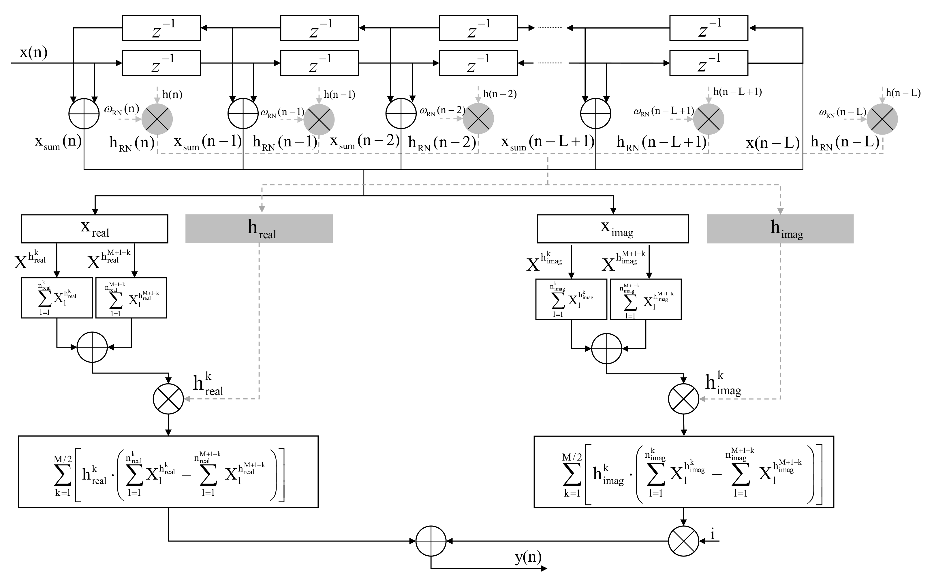
2.1. Time-Domain Equalization Implementation

The previous section shows that digital signal processing (DSP) is playing a growing role in the CDE. In digital coherent optical receivers, the CD transmission function of an optical pulse in the channel given by
G ( z , w ) = exp j D λ 2 4 π c ω 2 z
Here, D, z, λ , c and ω are dispersion coefficient, length of the fiber link, wavelength, light speed, and digital angular frequency. Therefore, we can derive an FD-FIR close to Equation (1) to compensation CD as
H Des e j ω T = 1 G ( z , ω ) = exp j D λ 2 4 π c ω 2 z
By implementing IFFT of Equation (2), the continuous CDE pulse response function as
g ( z , t ) = c j D λ 2 z exp ( j φ ( t ) ) , φ ( t ) = π c D λ 2 z t 2
Aliasing occurs when the digital angular frequency exceeds the Nyquist frequency determined by the sampling rate. To avoid aliasing, by direct sampling and truncation of Equation (3), we derived with a complex impulse response given by [17,18]
h ( k ) = jc T 2 D λ 2 z exp j π c T 2 D λ 2 z k 2 N 2 k N 2
Here, T is the sampling time. Where the length of the filter h ( k ) is the maximum number of filter taps so that aliasing does not occur, N is odd as
N = 2 × | D | λ 2 z 2 c T 2 + 1
where ⌊⌋ is the rounding down operation and | D | indicates absolute value. So we can further obtain the FD response of the filter after truncation as H ( k ) .
One of the drawbacks of Equation (4) is that truncation is applied to Equation (7) to avoid the aliasing of frequency. Still, truncation in the TD introduces energy leakage in the FD, so the main lobe of the window spectrum can only be approximated as a rectangle. Equation (4) has another drawback that the complexity of TD-CDE and FD-CDE are N 2 and N FFT log 2 N FFT , where N is the number of filter taps, and N FFT is the FFT block size. Therefore, for larger accumulated CD, such as in long-distance fiber transmission, the complexity of FD-CDE is lower than that of TD-CDE [19].

2.2. Optimize Time-Domain Equalization Implementation

With the continuous development of commercial coherent transceivers, higher efficiency requirements are put forward for the CDE algorithm to meet the requirements for power consumption. The previous TD-CDE method needs to be revisited to (I) improve the hardware implement ability of time CDE algorithms; (II) overcome the drawbacks mentioned above; (III) reduce dependence on subsequent adaptive equalization modules.

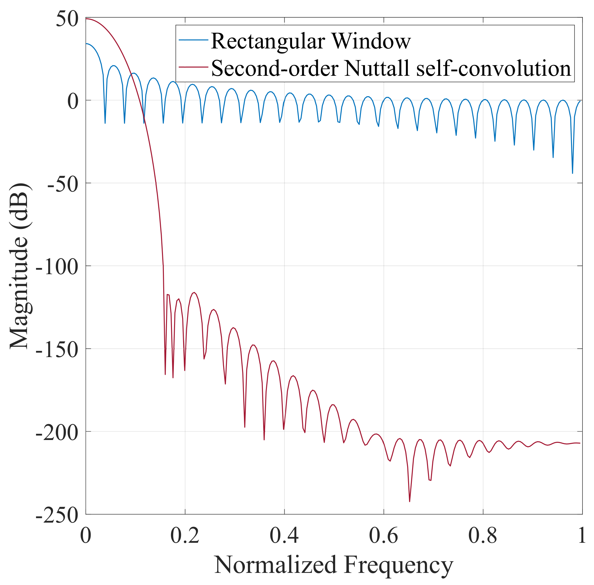
2.2.1. Window Function Weight Optimization

The frequency-domain response H Des e j ω T of an ideal filter has a constant amplitude-frequency characteristic in the passband. When the FD response of the designed filter is close to H Des e j ω T , the CDE effect is better, so the spectral energy of the window function is required to be concentrated on the main lobe as much as possible. The filtered spectrum H ( k ) obtained by the rectangular window truncation will have serious spectrum leakage, which is quite different from the ideal FD response H Des e j ω T . In this paper, based on the window function Nuttall window function with the smallest side lobe and fastest side lobe attenuation characteristics, considering that the four-term three-order Nuttall window has the fastest attenuation speed of side lobe compared to other window functions [20], the Nuttall second-order self-convolution window function is used.
The TD expression characteristics are
w R ( n ) = 1 , n = 1 , 2 , , N 0 , else
and its spectral characteristics are
W R ( ω ) = sin ( ω N / 2 ) sin ( ω / 2 ) exp j ω N 1 2
The Nuttall window is a combination window with good side lobe characteristics, and the TD expression is
ω N ( n ) = m M 1 ( 1 ) m c m cos ( 2 π n · m / N ) n = 1 , 2 N 1
Here, M is the number of terms of the window function, N is the length of the window function; C m is the coefficient, and satisfies the constraints
m = 0 M 1 ( 1 ) m c m = 0 , m = 0 M 1 c m = 1
and its spectral characteristics are
W N ( ω ) = m = 0 M 1 ( 1 ) m c m 2 W R ω 2 π m N + W R ω + 2 π m N
Here, W is the spectral function of the rectangular window. This paper selects a four-term three-order Nuttall window, the coefficients of which are c 1 = 0.338946 , c 2 = 0.481973 , c 3 = 0.161054 , c 4 = 0.018027 . The four-term three-order Nuttall window is self-convolved to obtain the second-order Nuttall self-convolution window function as
w RN ( n ) = w N ( n ) * w N ( n )
Time-frequency diagram of the rectangular window and second-order Nuttall self-convolution window function as shown in Figure 1.
It can be seen from the Figure that the side lobe performance of the Nuttall self-convolution window is significantly better than that of the rectangular window. Therefore, using the Nuttall self-convolution window to cut the signal can effectively suppress the spectrum leakage. The Nuttall self-convolution window function is used to window and truncate Equation (3) to obtain the CDE RN-FIR filter as
h RN ( n ) = ω RN ( n ) · h ( n ) , N 2 n N 2
After the signal is truncated in the TD with the window function, the FD amplitude of the signal will be affected, so amplitude restoration is required. The definition of the amplitude restoration coefficient h ( n ) is that the amplitude when other window functions are added is consistent with the amplitude of a rectangular window of the same length. Its expression is
K m = A 1 / A 2
Here, A 1 is the amplitude of the zero frequency point after adding a rectangular window, and A 2 is the amplitude of the zero frequency point after adding other windows. The modulus of the tap coefficient of the TD-CDE is constant, which limits the equalization effect. The above method is equivalent to using a window function to optimize the weight of the TD-CDE taps if there is no longer a constant value, which effectively improves the CDE filter effect.

2.2.2. Window Function Weight Optimization

In the convolution operation in the TD, the distribution characteristics of multiplication and the combination of addition are used to reduce the number of multiplication operations between input samples and tap quantization coefficients by implementing filter tap coefficient quantization, thereby reducing the computational complexity of TD-CDE. The uniform quantization method is used in the quantization process. As the number of quantization stages M decreases, the number of quantized values of filter tap coefficients decreases, and the system’s diversity increases. Figure 2 shows the schematic diagram of the real part of the tap coefficient before and after quantization; the quantization stages M is eight, and coefficients are normalized.
Before illustrating the specific implementation process, we must make two necessary explanations.
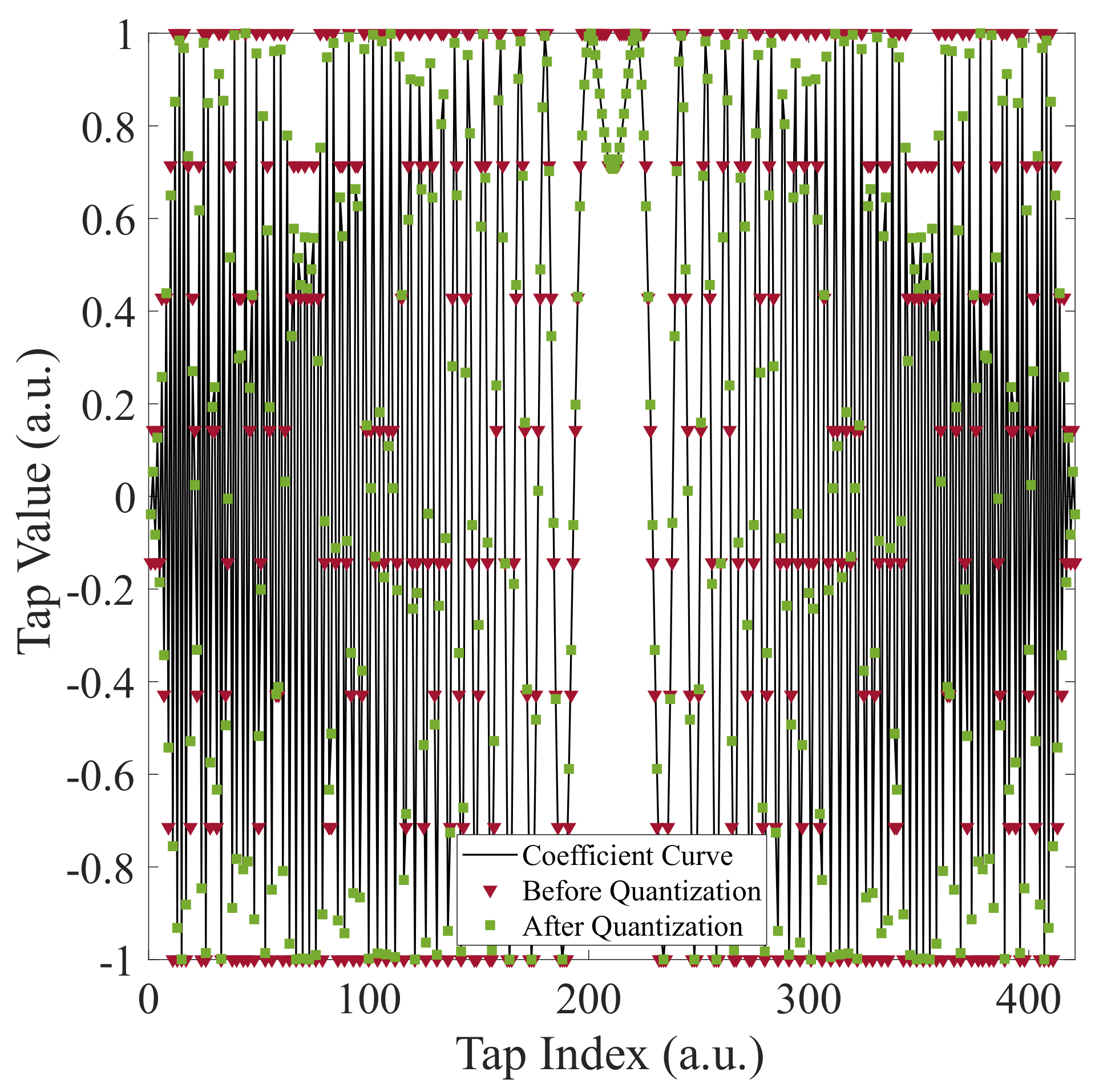
  • In this paper, the filter complex tap coefficients are independently written as their real and imaginary parts for operation. This operation can increase the diversity of filter tap coefficients, which is inversely proportional to the computational complexity of TD-CDE.
  • It can be seen from Equation (5) that the tap coefficient of the filter h ( k ) is symmetrical about the central coefficient [21]. Assuming the symmetric length is L, then L = N 1 2 . If the tap coefficients are uniformly quantized, the quantized value is also approximately symmetric about the central coefficient.
Through the above two points of analysis, before the tap coefficient quantization is implemented, the output value y ( n ) after equalization is
y ( n ) = m = 1 N x ( n + m 1 ) h ( N m + 1 )
among them, the filter coefficient h ( N i + 1 ) can be written in the form of the real part plus the imaginary part, as shown below
h ( N m + 1 ) = h real ( N m + 1 ) + h imag ( N m + 1 ) · i , m = 0 , 1 , 2 , , N
Therefore, from Equations (14) and (15), the output value y ( n ) can be written as two parts y 1 ( n ) and y 2 ( n ) , which are
y 1 ( n ) = m = 1 N x ( n + m 1 ) h real ( N m + 1 ) y 2 ( n ) = m = 1 N x ( n + m 1 ) h imag ( N m + 1 ) · i
Performing uniform quantization on the filter coefficients, the quantization level is M. Taking the real part h real ( N m + 1 ) of the filter coefficient as an example, it is quantized into M levels. The real part of the filter coefficient after quantizing can be expressed as h real k , k = 1 , 2 , , M , and the number of each level is n real k . After the above operation, the input digital signal can be preprocessed using binding law to reduce the complexity of subsequent calculations. Taking h real k as an example, combining the application of multiplication distribution and addition combination can extract the common factor h real k for n real k times of multiplication operations, and accumulate the sum value of the input sequence X h real k with the same common factor h real k is l = 1 n real k X l h real k . The calculation method is changed from the accumulative after polynomial multiplication to multiplication after the polynomial accumulative, which can get l = 1 n real k X l h leal k · h real k . Because uniform quantization is adopted, the filter coefficients after quantization have the following properties
h real k = h real M + 1 k
The calculation can be further simplified as shown
y 1 h real k ( n ) = l = 1 n real k X l h real k l = 1 n real M + 1 k X l h real M + 1 k · h real k
In the same way, the calculation results of the second part areas are
y 2 h imag k ( n ) = l = 1 n imag k X l h imag k l = 1 n imag M + 1 k X l h imag M + 1 k · h imag k · i
In summary, the CDE filter h ( n ) and the output value y ( n ) are
h real ( n ) h real k 0 k M / 2 , N 2 n N 2 h imag ( n ) h imag k · i 0 k M / 2 , N 2 n N 2 y ( n ) = k = 1 M / 2 h real k · l = 1 n real k X l h real k l = 1 n real M + 1 k X l h real M + 1 k + k = 1 M / 2 h imag k · l = 1 n imag k X l h imag k l = 1 n imag M + 1 k X l h imag M + 1 k · i
The detailed calculation flow for each sample of equalized output is shown in Figure 3.
Next, we will analyze the calculation workload before and after the quantization of the filter tap coefficients. The computational complexity evaluation is based on real number adders R add and real number multipliers R mul . The computational complexity of subtraction is the same as addition, so subtraction counts as addition in the complex calculation. Implementing a complex adder C add requires two R add , while a complex multiplier C mul only requires three R mul and five R add . The implementation process is
Z 1 = a + b · i , Z 2 = c + d · i Z 1 · Z 2 = ( a + b ) ( c d ) + a · d b · c + ( a · d + b · c ) · i
First, analyze the complexity of the TD-CDE. It can be seen from Equation (5) that the number of filter taps is an odd number N. For each equalized output value, it needs to perform N · C mul and ( N 1 ) · C add , which are converted into real number multiplication and real number addition
n R mul = 3 · N n R add = 7 · N 2
From Equation (21), it can be concluded that the times of complex number addition and complex number multiplication of the TD-CDE after quantization are
n R add = 2 · k = 1 M / 2 n real k + n real M + 1 k + n imag k + n imag M + 1 k 2 + 2 · M = 4 · N 4 + 2 · M n R mul = 2 · M

3. Simulation and Analysis

3.1. Environment

To verify the effectiveness of the proposed algorithm, the software Optisystem 15 is used to build a coherent optical communication system, and MATLAB components are used to realize DSP, as shown in Figure 4.
The system adopts a square root raised cosine (SRRC) pulse signal generator at the transmitter and SRRC filter at the receiver for matched filtering. The fiber link is composed of optical fibers, optical amplifiers (OA), an optical filter, and a loop controller, in which the span length is 100 km, the noise figure is 6 dB and the gain compensation is 20 dB. ADC samples the sequence at twice the symbol rate before sending the sequence to the MATLAB component to complete DSP. Table 1 is the system parameter setting.

3.2. Result Simulation

In this chapter, we will evaluate the impact of filter tap weight optimization and coefficient quantization on the performance of CDE in multiple formats compared with TD-CDE and FD-CDE, such as Equations (2) and (4). The FD-CDE adopts the method proposed in [7].

3.2.1. Weight Optimization Performance Analysis

Set the optical signal modulation format to DP-QPSK and DP-16QAM, analyze the effects of the optical signal to noise ratio (OSNR) to TD-CDE and FD-CDE, with weight-optimized time-domain chromatic dispersion equalization (WO-TD-CDE), such as Equation (12). The comparison is mainly reflected in two categories; the first is the longitudinal comparison to three kinds of filters, and the second is the transverse comparison to the same kind of filter. The control variable method is used to ensure that the simulation experiment is based on fairness. The variable in the first type of comparison is the CDE algorithm in DSP, and the variable in the second type of comparison is the length of the optical fiber link. Each test independently repeats thirty times to reduce random errors, as shown in Figure 5.
From Figure 5, we can observe that the equalization performance of the filter in Equation (12) is better than that in Equations (2) and (4), which is more prominent in short–medium distance transmission and high OSNR, as shown in Figure 5a. The performance advantage of Equation (12) is greater under the high-order modulation format in Figure 5b. Therefore, using the second-order Nuttall self-convolution window function to optimize the weight of the filter coefficients can effectively improve the CDE effect of a short–medium distance coherent optical communication system, which is also suitable for long-distance transmission systems under high OSNR.

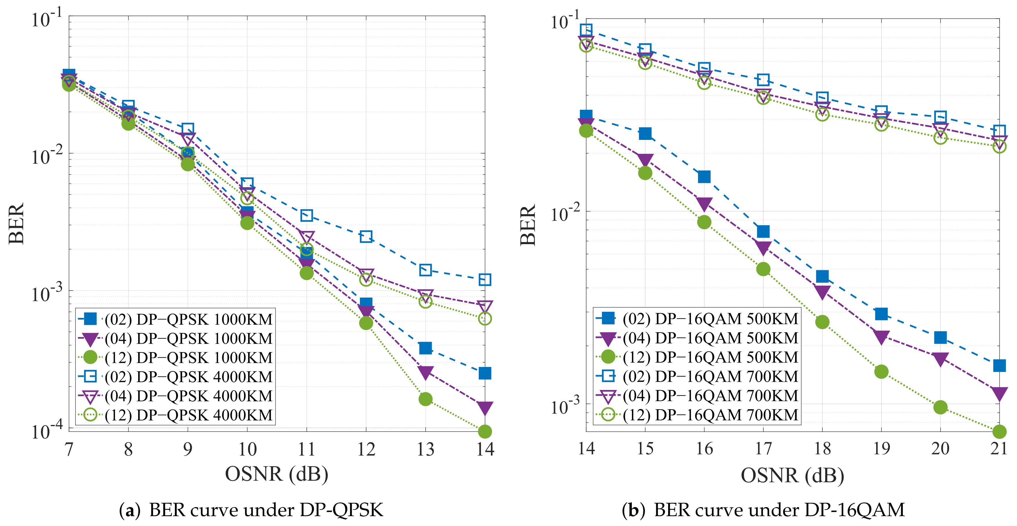
3.2.2. Coefficient Quantification Performance Analysis

Under different fiber transmission distances, we consider multiple quantization levels M, compare the CDE performance of the filter in Equation (4) and the filter in weight-optimized coefficient quantization time-domain chromatic dispersion equalization (CQWO-TD-CDE), such as Equation (20), and study the dependence of BER on the transmission distance of several filters and the influence of the quantization level M on the performance of the filter. In a real link, the signal OSNR is dependent on the link length, and the OSNR required to reach a certain BER level is analyzed. However, in the simulation experiment in this article, we consider the difference of BER under the same OSNR. Therefore, we added the setup OSNR component after the fiber link transmission in the simulation system to add a defined noise floor level to the signal. Figure 6a,b depict the four filters’ performance under DP-QPSK and DP-16QAM modulation, with the OSNR of 15 dB and 21 dB, respectively. From the Figure, we can find that as the number of quantization stages M increases, the filter’s performance in Equation (20) is close to the filter in Equation (4). To quantitatively analyze the performance loss caused by quantization, we introduce the quality factor Q, which is defined as the ratio of the difference between the BER before and after quantization to the BER before quantization. Its expression is
Q = B E R CQWO - TD - CDE B E R TD - CDE / B E R TD - CDE
The larger the Q, the greater the performance loss caused by quantization. Figure 6c,d show the relationship between quality factor Q and transmission distance under different quantization stages M.

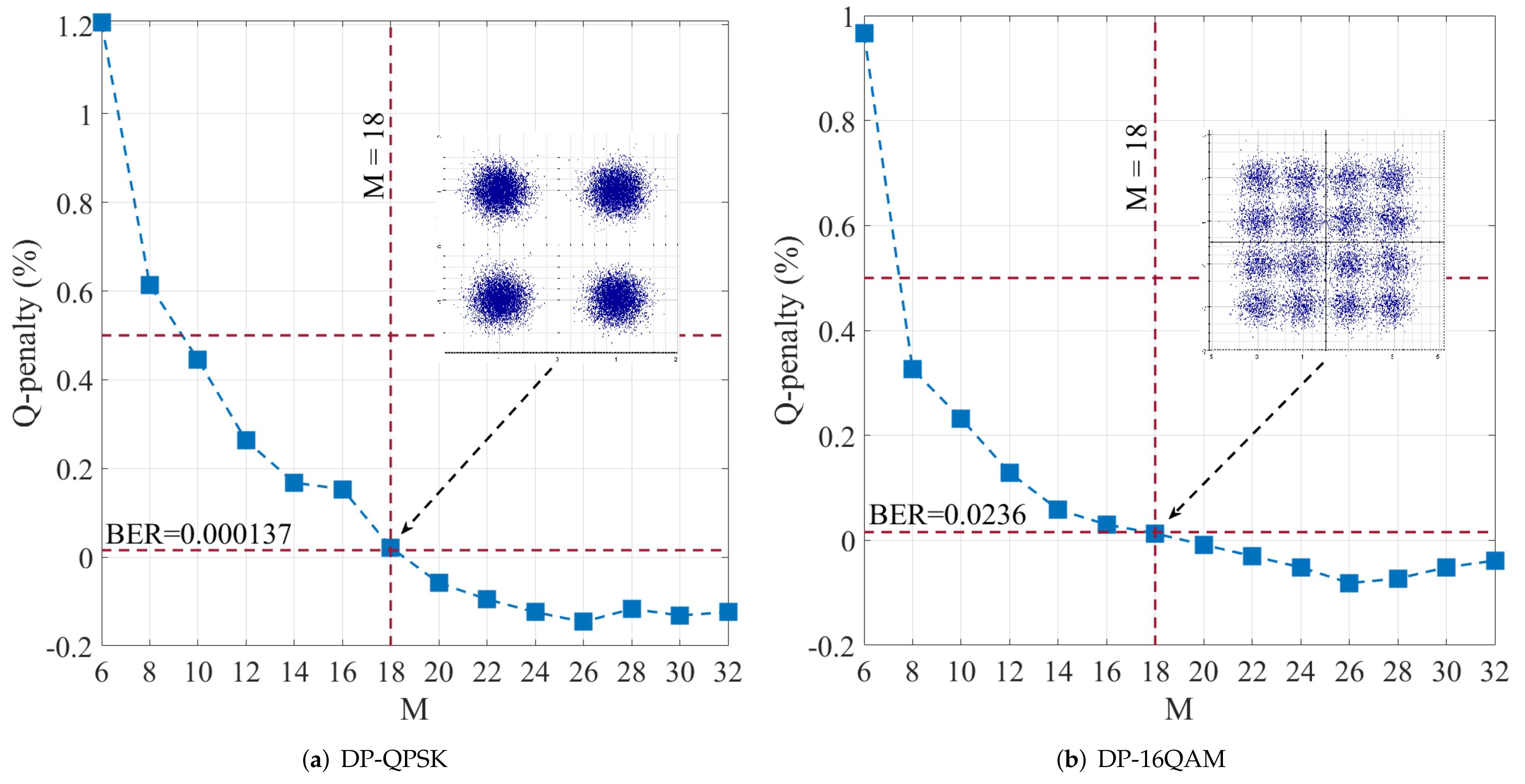
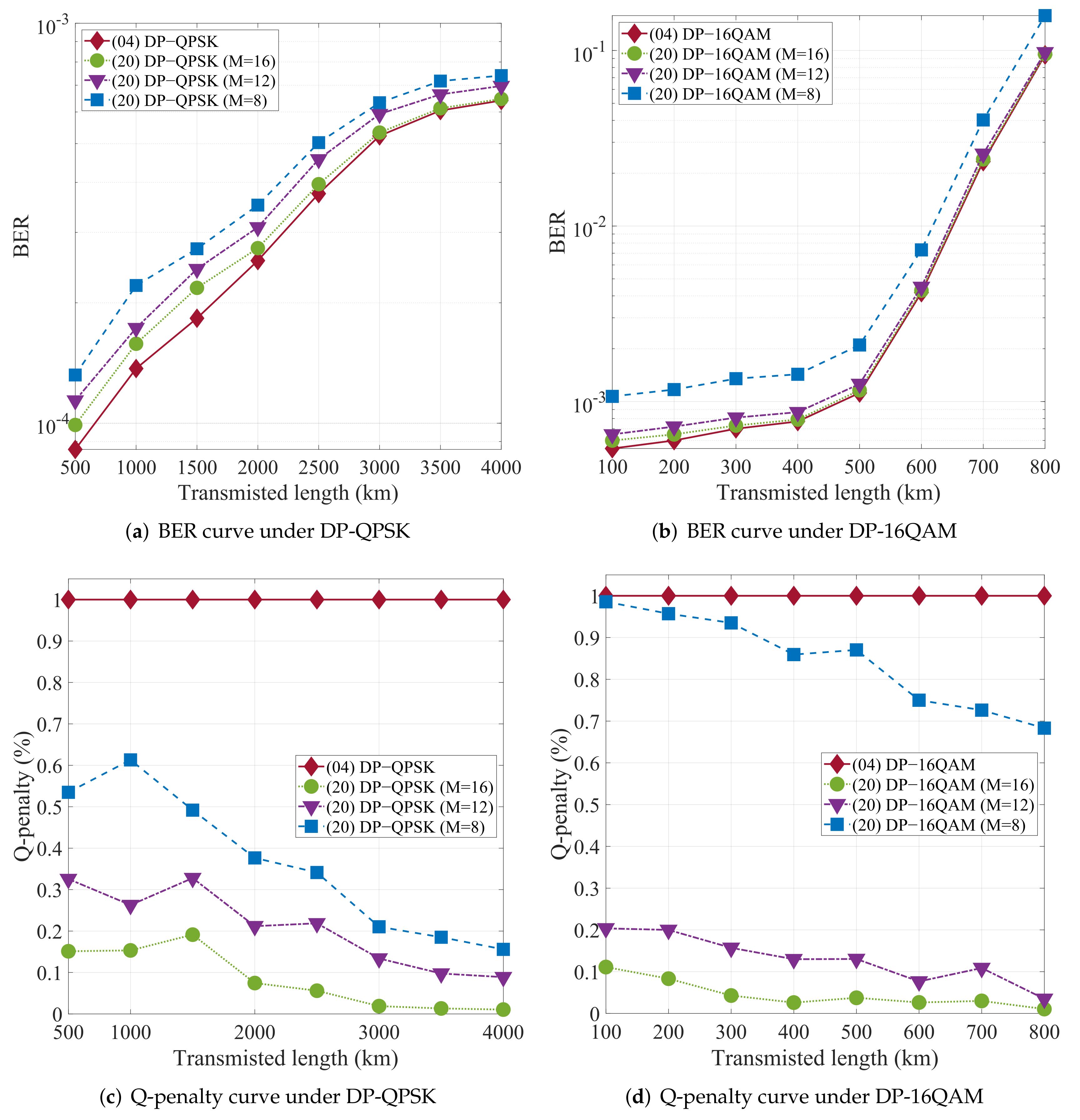
3.2.3. Coefficient Quantification and Q-Penalty

As we observed in the previous chapter, the Q value decreases and becomes more stable as the quantization stage M increases. Therefore, we assume that Q deteriorates to 50% as the threshold to verify the required quantization stage M. the modulation formats are DP-QPSK and DP-16QAM. The transmission distance is 1000 km and 700 km, and the OSNR is 15 dB and 21 dB, respectively. The rest of the simulation conditions remain unchanged, and the relationship curve between the quality factor Q and the quantization stage M is shown in Figure 7.
It can be seen that as the number of quantization stage M increases, the quality factor Q also gradually decreases. Whether it is in DP-QPSK or DP-16QAM modulation, when M is greater than 10, the Q value drops below 50%. When M exceeds 18, the Q becomes a negative number, and it can be seen from Equation (24) that the BER of the CQWO-TD-CDE is lower than that of the TD-CDE. The higher the quantization stage M, the closer the performance of the CQWO-TD-CDE is to that of the WO-TD-CDE, which means that under this condition, the performance of CQWO-TD-CDE exceeds TD-CDE, and Q tends to stabilize at about −10%.

4. Discussion

This section compares the calculated workload of CQWO-TD-CDE, TD-CDE, and FD-CDE. When calculating complexity in CQWO-TD-CDE, it is necessary to consider window function weight optimization. The comparison content for (I) each equalized output value needs real number multiplication n R mul and real number addition n R add ; (II) total amount of calculation in the equalization process about real number multiplication n R mul T and real number addition n R add T . To facilitate quantitative comparison of the calculation operations between different equalizers, a constant factor η mul and η add is introduced, and the expression is
η mul = 1 n R mul T 1 / n R mul T 2 η add = 1 n R ddd T 1 / n R add T 2
Here, η mul and η add are the optimizations indexed of the proposed algorithm to calculate the operands, η mul is the real number multiplication calculation, and η add is the real number addition calculation. The larger η mul and η add , the lower the computational complexity of the proposed algorithm. n R mul T 1 and n R add T 1 are the total calculation times of real number multiplication and real number addition in the experimental group (CQWO-TD-CDE). n R mul T 2 and n R add T 2 are the full calculation times of real number multiplication and real number addition in the control group (TD-CDE or FD-CDE).

4.1. Comparision of TD-CDE and CQWO-TD-CDE

As analyzed in Section 3, for TD-CDE, the calculation amount of real number multiplication and the addition calculation amount of each equalized sample output depends on the number of filters taps N. In the CQWO-TD-CDE, the calculation amount of real number multiplication is only related to the quantization stages M, and the degree of correlation between the calculation amount of real number addition and the filter taps N is also lower than that of TD-CDE. Considering different quantization stages M, the quantitative analysis of the changing trend of η mul and η add is shown in Table 2.
From the analysis in Table 2, we find that when the fiber transmission distance is fixed, as the quantization stages increase, the computational complexity of the optimized algorithm will increase slightly. Still, the computation complexity of the real number multiplication η mul can also reduce by more than 90%. From Section 3, we can see that the increase in the quantization order can significantly improve the algorithm’s performance. When the quantization stage M is fixed, as the transmission distance increase, the computational complexity of the optimized algorithm decreases. In summary, the proposed optimization algorithm can greatly reduce the computational workload under long-distance and large CD conditions. Even considering the performance requirements to compromise and the quantization stages are set to M = 16 , the optimization indexes η mul and η add also show efficient optimization.

4.2. Comparision of FD-CDE and CQWO-TD-CDE

From Section 3, we know that the computational complexity of FD-CDE is proportional to the size of the FFT block N FFT In the optical communication system of long-distance transmission from cost, FD-CDE is far superior to TD-CDE. Therefore, CQWO-TD-CDE must be compared with FD-CDE to evaluate the replaceability. In the overlap preservation method, the N FFT size signal block is transformed into the FD through FFT, then multiplied by the transmission function of the dispersion equalization filter, and then transformed into the TD through IFFT. An FFT operation includes N FFT / 2 · log 2 N FFT times of complex number multiplication operations and N FFT · log 2 N FFT times of complex number addition operations. It can be calculated that in FD-CDE, the real number multiplication and real number addition required for each, equalized, are
n R mul = 3 · N FFT · log 2 N FFT + N FFT n R add = 9 · N FFT · log 2 N FFT + 5 · N FFT
The overlap value in FD-CDE is the key parameter determined by CD. As long as an integer is greater than the necessary overlap, it can theoretically be used as the N FFT . However, for different CD values, there is an optimal N FFT to achieve the optimal calculation amount of FD-CDE, and as the CD value increases, the optimal N FFT also increases. The optimal N FFT used in the experiment comes from [22] The overlap size is specified as half of the N FFT to simplify the calculation. Considering that the multiplication module is the most important indicator of the complexity in the digital signal processing module, we mainly compare the multiplication operations in FD-CDE and CQWO-TD-CDE, as shown in Figure 8.
The results in Figure 8 prove that in long-distance optical fiber communication, the computational complexity of CQWO-TD-CDE is still better than that of FD-CDE. With the increase in optical fiber distance, this advantage presents an upward trend. The lower the quantization level M, the better performance optimization. When M = 8 and the optical fiber distance is 4000 km, the calculation complexity optimization reaches more than 60%; even in the short-distance optical fiber communication, such as 200 km, the performance index is also close to 35%. If weighting the performance requirements, such as setting the quantization level M = 16, when the fiber distance is 4000 km, the calculation complexity is also close to 30% optimization.

5. Conclusions

This paper uses a Nuttall second-order self-convolution window with the smallest side-lobe peak value and the fastest side-lobe attenuation rate. The uniform quantization of tap coefficients results in a high diversity of real and imaginary parts; a low complexity TD-CDE for DSP is proposed. Using Optisystem 15 to build a coherent optical communication system for simulation verification, the following three points have been obtained. (I) Compared with rectangular windows, a Nuttall second-order self-convolution window is used to optimize the weight of the TD-CDE filter, which can effectively reduce the effect energy leakage caused by the truncation effect. (II) Compared with the standard TD-CDE, by using a Nuttall second-order self-convolution window function to optimize the weight of the filter, and then uniformly quantifying the filter coefficient, rationally using the multiplication distribution law, addition combination law, and the symmetry of the filter coefficients, while maintaining equalization performance, the demand for multipliers and adders in the convolutional operation process can be greatly reduced, and it is more suitable for commercial coherent optical communication systems. The real number multiplication operation reduces by 99%, the real number addition operation reduces by 43%, and the performance only reduces by 5% when the quantization coefficient M = 16. (III) From the analysis of the quality factor Q in Section 3 and the constant-coefficient η mul in Section 4, it can be seen that in the long-distance optical fiber link, considering the certain equilibrium performance loss, the proposed CQWO-TD-CDE method can be reduced by more than 60% compared with the commonly used FD-CDE method, and the optimization effect is highlighted with the increase in the transmission distance, effectively reducing the complexity of the hardware implementation of commercial coherent receivers.
In general, it has been proven that the proposed equalizer can achieve the double guarantee of performance and computational complexity. It can become an effective alternative to FD-CDE in long-distance fiber communication.

Author Contributions

Conceptualization, Z.W. and Z.H.; methodology, Z.W.; software, Z.W.; supervision, Z.H.; valida-tion, S.L.; writing (original draft), Z.W.; data curation, F.S.; writing, review and editing, Y.Z.; All authors have read and agreed to the published version of the manuscript.

Funding

This research was supported by Nation Natural Science Foundation of China, grant number 51575517 and Natural Science Foundation of Hunan Province, grant number 2019JJ50121.

Institutional Review Board Statement

Not applicable.

Informed Consent Statement

Not applicable.

Data Availability Statement

Not applicable.

Acknowledgments

The authors would like to thank the editors and anonymous reviewers for giving valuable suggestions that have helped to improve the quality of the manuscript.

Conflicts of Interest

The authors declare no conflict of interest.

References

  1. Charlet, G.; Pecci, P. 5—Ultra-long haul submarine transmission. In Undersea Fiber Communication Systems, 2nd ed.; Academic Press: Cambridge, MA, USA, 2016; Volume 10, pp. 165–235. [Google Scholar]
  2. Wang, D.; Jiang, H.; Liang, G.; Zhan, Q.; Su, Z.; Li, Z. Chromatic dispersion equalization FIR filter design based on discrete least-squares approximation. Opt. Express 2021, 29, 20387–20394. [Google Scholar] [CrossRef] [PubMed]
  3. Xiang, Z.; Nelson, L.E. 400G WDM Transmission on the 50 GHz Grid for Future Optical Networks. J. Light. Technol. 2012, 30, 3779–3792. [Google Scholar]
  4. Xu, T.; Jin, C.; Zhang, S.; Jacobsen, G.; Liu, T. Phase Noise Cancellation in Coherent Communication Systems Using a Radio Frequency Pilot Tone. Appl. Sci. 2019, 9, 4717. [Google Scholar] [CrossRef] [Green Version]
  5. Zhao, J.; Liu, Y.; Xu, T. Advanced DSP for Coherent Optical Fiber Communication. Appl. Sci. 2019, 9, 4192. [Google Scholar] [CrossRef] [Green Version]
  6. Kuschnerov, M.; Hauske, F.N.; Piyawanno, K.; Spinnler, B.; Alfiad, M.S.; Napoli, A.; Lankl, B. DSP for Coherent Single-Carrier Receivers. J. Light. Technol. 2009, 27, 3614–3622. [Google Scholar] [CrossRef] [Green Version]
  7. Geyer, J.C.; Fludger, C.R.S.; Duthel, T.; Schulien, C.; Schmauss, B.J.I. Efficient Frequency Domain Chromatic Dispersion Compensation in a Coherent Polmux QPSK-Receiver. In Proceedings of the 2010 Conference on Optical Fiber Communication (OFC/NFOEC), Collocated National Fiber Optic Engineers Conference, San Diego, CA, USA, 21–25 March 2010; Wiley Telecom: Washington, DC, USA, 2010; pp. 1–3. [Google Scholar]
  8. Felipe, A.; de Souza, A.L. Chirp-Filtering for Low-Complexity Chromatic Dispersion Compensation. J. Light. Technol. 2020, 38, 2954–2960. [Google Scholar] [CrossRef]
  9. Pillai, B.S.G.; Sedighi, B.; Guan, K.; Anthapadmanabhan, N.P.; Shieh, W.; Hinton, K.J.; Tucker, R.S. End-to-End Energy Modeling and Analysis of Long-Haul Coherent Transmission Systems. IEEE/OSA J. Light. Technol. 2014, 32, 3093–3111. [Google Scholar] [CrossRef]
  10. Kachris, C.; Tomkos, I. A Survey on Optical Interconnects for Data Centers. IEEE Commun. Surv. Tutor. 2012, 14, 1021–1036. [Google Scholar] [CrossRef]
  11. Ohlen, P.; Skubic, B.; Rostami, A.; Fiorani, M.; Monti, P.; Ghebretensae, Z.; Martensson, J.; Kun, W.; Wosinska, L. Data Plane and Control Architectures for 5G Transport Networks. J. Light. Technol. 2015, 34, 1501–1508. [Google Scholar] [CrossRef]
  12. Zhu, Y.; Plant, D.V. Optimal Design of Dispersion Filter for Time-Domain Split-Step Simulation of Pulse Propagation in Optical Fiber. J. Light. Technol. 2012, 30, 1405–1421. [Google Scholar] [CrossRef]
  13. Vorapoj, P. Performance Analysis of Digital FIR LP Filter Implementation based on 5 Window Techniques: Rectangular, Barlett, Hann, Hamming and Blackman. Int. J. Simul. Syst. 2019, 20, 1111–1116. [Google Scholar]
  14. Wu, Z.; Lei, L.; Dong, J.; Zhang, X. Triangular-shaped pulse generation based on self-convolution of a rectangular-shaped pulse. Opt. Lett. 2014, 39, 2258–2261. [Google Scholar] [CrossRef] [PubMed]
  15. Wen, H.; Teng, Z.; Guo, S.; Wang, J.; Yang, B.; Wang, Y.; Chen, T. Hanning self-convolution window and its application to harmonic analysis. Sci. China Ser. E Technol. Sci. 2009, 52, 467–476. [Google Scholar] [CrossRef]
  16. Wen, H.; Zhang, J.; Meng, Z.; Guo, S.; Li, F.; Yang, Y. Harmonic Estimation Using Symmetrical Interpolation FFT Based on Triangular Self-Convolution Window. IEEE Trans. Ind. Inf. 2015, 11, 16–26. [Google Scholar] [CrossRef]
  17. Eghbali, A.; Johansson, H.; Gustafsson, O.; Savory, S.J. Optimal Least-Squares FIR Digital Filters for Compensation of Chromatic Dispersion in Digital Coherent Optical Receivers. J. Light. Technol. 2014, 32, 1449–1456. [Google Scholar] [CrossRef]
  18. Zhou, X.; Xie, C. Enabling Technologies for High Spectral-Efficiency Coherent Optical Communication Networks; Wiley Telecom: Washington, DC, USA, 2016; pp. 13–64. [Google Scholar]
  19. Spinnler, B. Equalizer Design and Complexity for Digital Coherent Receivers. IEEE J. Sel. Top. Quantum Electron. 2010, 16, 1180–1192. [Google Scholar] [CrossRef]
  20. Zhang, D.; Sun, S.; Zhao, H.; Yang, J. Laser Doppler signal processing based on trispectral interpolation of Nuttall window. Optik 2020, 205, 163364. [Google Scholar] [CrossRef]
  21. Xu, T.; Jacobsen, G.; Popov, S.; Li, J.; Vanin, E.; Wang, K.; Friberg, A.T.; Zhang, Y. Chromatic dispersion compensation in coherent transmission system using digital filters. Opt. Express 2010, 18, 16243–16257. [Google Scholar] [CrossRef] [PubMed] [Green Version]
  22. Xu, T.; Jacobsen, G.; Popov, S.; Forzati, M.; Mårtensson, J.; Mussolin, M.; Li, J.; Wang, K.; Zhang, Y.; Friberg, A.T. Frequency Domain Chromatic Dispersion Equalization Using Overlap-Add Methods in Coherent Optical System. J. Opt. Commun. 2011, 32, 131–135. [Google Scholar] [CrossRef]
Figure 1. Side lobe performance of second-order Nuttall self-convolution window and rectangular window.
Photonics 09 00263 g001
Figure 2. The real part of exact and quantized coefficients for M = 8 and N = 415 .
Photonics 09 00263 g002
Figure 3. Symmetric CQWO-TD-CDE FIR filter architecture.
Photonics 09 00263 g003
Figure 4. Coherent optical communication system structure diagram.
Photonics 09 00263 g004
Figure 5. The BER performance of the DP-QPSK and DP-16QAM data. We compare the TD-CDE FIR filter, FD-CDE FIR filter, and WO-TD-CDE FIR filter under different OSNR. (a) Under the DP-QPSK modulation format, the fiber transmission distance is 1000 km and 4000 km, respectively. (b) Under the DP-16QAM, the fiber transmission distance is 500 km and 700 km, respectively.
Photonics 09 00263 g005
Figure 6. The BER and Q-penalty performance of the DP-QPSK and DP-16QAM data. We compare the filters of the TD-CDE FIR filter and the CQWO-TD-CDE FIR filter under different transmission distances. (a) BER curve under the DP-QPSK; the fiber transmission distance is from 500 km to 4000 km, respectively. (b) BER curve under the DP-QPSK; the fiber transmission distance is from 100 km to 800 km. (c) Q-penalty curve under the DP-QPSK; the fiber transmission distance is from 500 km to 4000 km. (d) Q-penalty curve under the DP-16QAM; the fiber transmission distance is from 100 km to 800 km.
Photonics 09 00263 g006
Figure 7. The Q-penalty performance of the DP-QPSK and DP-16QAM data. We compare the filters of the TD-CDE FIR filter and the CQWO-TD-CDE FIR filter under different quantization stages M. (a) Q-penalty curve under the DP-QPSK, and the fiber transmission distance is 1000 km. (b) Q-penalty curve under the DP-16QAM and the fiber transmission distance is 700 km.
Photonics 09 00263 g007
Figure 8. The influence of fiber transmission distance on the optimization performance of real number multiplication under different quantization stages M.
Photonics 09 00263 g008
Table 1. System simulation parameter.
ParameterValueParameterValue
Wavelength1550 nmChromatic dispersion coefficient16.5 ps/nm/km
Sequence length131,072Group velocity dispersion coefficient0.2 ps/km
Symbol rate28 GBaudLaser line width0.1 MHz
Modulation formatQPSK/16QAMAttenuation coefficient0.2 db/km
Roll-off factor0.25/1Signal power10 dbm
Table 2. The degree of correlation between the calculation amount of real number multiplication η mul and real number addition η add and quantization stages M.
L/km50010001500
N207415623
M812168121681216
η mul 97.496.194.898.798.197.499.198.798.3
η add 41.941.440.842.442.141.942.642.242.2
Publisher’s Note: MDPI stays neutral with regard to jurisdictional claims in published maps and institutional affiliations.

