Cavity-Enhanced Frequency Comb Vernier Spectroscopy

 ,
,
Abstract
:1. Introduction
2. Principles of Vernier Filtering
2.1. Comb–Cavity Coupling at Perfect Match
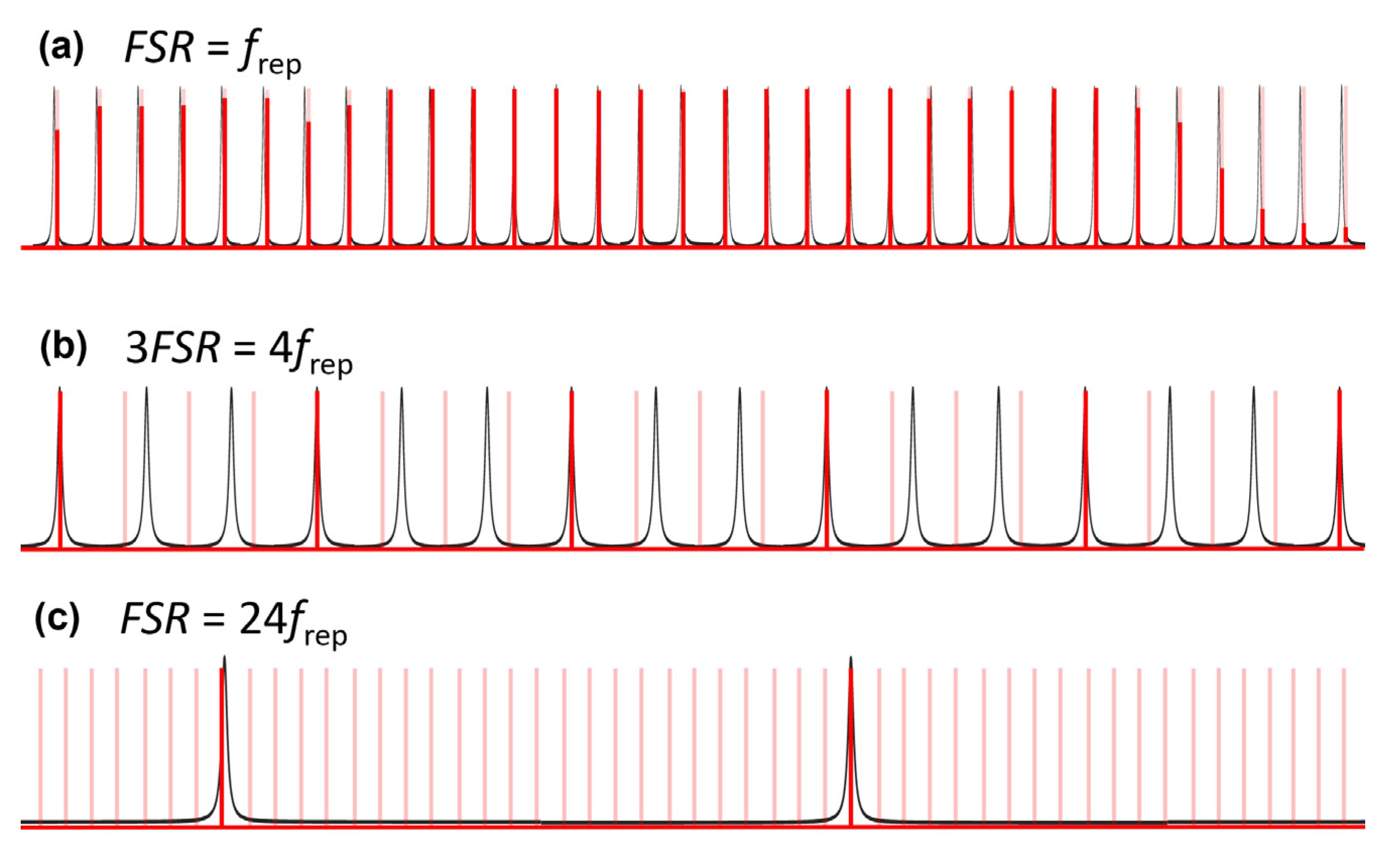
2.2. Comb-Resolved Filtering
2.3. Continuous Filtering
3. Previous Demonstrations

| Paper | Laser Source and frep | Range | Cavity Finesse, FSR and Vernier Ratio | Sensitivity | Target Species | Detection Scheme |
|---|---|---|---|---|---|---|
| [8] 2007 | Ti:sapphire 1 GHz | 4 THz @ 0.785 µm | F = 3000 FSR = 1 GHz m/q = 69/68 | NEA = 5 × 10⁻⁶ cm−1 @ 10 ms 4000 elements | O2 in cavity | Figure 3a |
| [23] * 2014 | Er:fiber 250 MHz | 5 THz @ 1.53 µm | F = 30,000 FSR = 250 MHz m/q = 500/499 | NEA = 8 × 10⁻⁸ cm−1 @ 1 s FoM = 1.2 × 10⁻⁹ cm−1 Hz−1/2 | C2H2 in cavity | Figure 3a |
| [15] † 2015 | Er:fiber + Tm-Ho amp. 250 MHz | 0.032 THz @ 2 µm | F = 100 FSR = 4.5 GHz m/q = 18/1 | Not reported | CO2 in cavity | Figure 3a |
| [24] † 2018 | Same as above | 1.8 THz @ 1.96 µm 0.03 THz steps | Same as above | Not reported | CO2 in cavity | Figure 3a |
| [25] † 2021 | Tm:fiber 400 MHz | 0.15 THz @ 1.97 µm | F = 200 FSR = 6.25 GHz m/q = 25/1 | Not reported | 12/13CO2 in cavity | Figure 3a |
| [26] 2014 | Ti:sapphire-pumped intracavity DFG 1 GHz | 0.2 THz @ 4.33 µm | F = 8000 FSR = 150 MHz m/q = 3/20 | Not reported | CO2 in 2 m air path | Single InSb detector |
| [18] 2015 | Er:fiber 250 MHz | 4 THz @ 1.543 µm | F = 200 FSR = 9.5 GHz m/q = 38/1 | FoM‡ = 2.6 × 10⁻⁵ cm−1 Hz−1/2 | H13C14N in 0.5 cm cell | Figure 3b |
| [16] † 2019 | Er:fiber 250 MHz | 1.7 THz @ 1.578 µm | F = 18,000 FSR = 267 MHz m/q = 16/15 | NEA ** = 1 × 10⁻⁸ cm−1 @ 2000 s | CO in cavity †† | Figure 3b |
| [27] 2016 | Er:fiber 250 MHz | 0.85 THz @ 1.53 µm 0.12 THz steps | F = 300 FSR = 1 GHz m/q = 4/1 (or higher) | NEA§ = 8.45 × 10⁻⁴ cm−1 @ 0.1 s | C2H2 in 14.2 cm cell | Fiber spectrometer |
| [28] † 2016 | Er:fiber 250 MHz | 3 THz @ 1.55 µm 1 THz steps | F = 50,000 FSR = 1 THz m/q = 400/1 | FoM = 2.7 × 10⁻⁹ cm−1 Hz−1/2 | C2H2 in 33 m multipass cell | Figure 3c |
| [17] † 2020 | Er:fiber 250 MHz | 4 THz @ 1.53 µm | F = 50,000 FSR = 600 GHz m/q = 2400/1 | Not reported | C2H2 in 10 cm cell§§ | Figure 3c |
| [29] 2022 | GaSb-based ICL 9.7 GHz | 1 THz @ 3.636 µm | F = 3050 FSR = 4.83 GHz m/q =250/502 | NEA = 7.8 × 10⁻⁶ cm−1 @ 1 s | HFC-152a–1,1-Difluoroethane in cavity | Figure 3d |
| Paper | Laser Source and frep | Range and Resolution | Cavity Finesse and FSR | Sensitivity | Target Species | Detection Scheme |
|---|---|---|---|---|---|---|
| [10] 2008 | Er:fiber 99 MHz | 3.2/1.6 THz @ 1.525 µm ΓV = 10/5 GHz | F = 6300 FSR = 396 MHz | Not reported | C2H2 | Single InGaAs detector |
| [9] 2014 | Ti:sapphire 90 MHz | 39 THz @ 0.79 µm ΓV = 4/1 GHz | F = 300 FSR = 90 MHz | NEA = 1.7 × 10⁻⁸ cm−1 @ 100 ms FoM = 6 × 10⁻¹¹ cm−1 Hz−1/2 | O2 and H2O in air | Figure 4a |
| [20] 2017 | Ti:sapphire 90 MHz | 60 THz @ 0.79 µm ΓV = 2 GHz | F = 3000 FSR = 90 MHz | NEA = 2 × 10⁻⁸ cm−1 @ 1 s FoM = 1.1 × 10⁻¹⁰ cm−1 Hz−1/2 | O2 and H2O in air | Figure 4a |
| [31] 2016 | Tm:fiber-pumped OPO 125 MHz | 11 THz @ 3.2 µm (in 16 steps) ΓV = 10 GHz | F = 300 FSR = 250 MHz | NEA = 6.2 × 10⁻⁷ @ 2 ms FoM = 3.3 × 10⁻⁹ cm−1 Hz−1/2 | H2O and CH4 in air | Grating and single HgCdTd detector |
| [22] 2017 | Tm:fiber-pumped OPO 125 MHz | 7.2 THz @ 3.25 µm ΓV = 7–8 GHz | F = 300 FSR = 250 MHz | NEA = 5.2 × 10⁻⁸ cm−1 @ 1 s FoM = 1.7 × 10⁻⁹ cm−1 Hz−1/2 | CH4 and H2O in air | Figure 4a |
| [32] 2019 | Er:fiber 250 MHz | 1.6 THz @ 1.57 µm ΓV = 6.6 GHz | F = 760 FSR = 250 MHz | NEA = 4 × 10⁻⁷ cm−1 @ 25 ms FoM = 2.6 × 10⁻⁸ cm−1 Hz−1/2 for 3.8 cm flame diameter | H2O and OH in a flame | Figure 4a |
| [33] 2020 | Er:fiber 125 MHz | 1.2 THz @ 1.578 µm ΓV = 4.4 GHz | F = 1050 FSR = 250 MHz | NEA = 5.5 × 10⁻⁸ cm−1 @ 50 ms FoM = 7.4 × 10⁻¹⁰ cm−1 Hz−1/2 | CO2 in air | Figure 4a |
| [21] 2021 | Er:fiber 125 MHz | 1.7 THz @ 1.575 µm ΓV = 6.6 GHz and 2.7 THz @ 1.650 µm ΓV = 13 GHz | @ 1575 nm F = 760 and @ 1650 nm F = 370 FSR = 250 MHz | @ 1575 nm NEA = 5 × 10⁻⁹ cm−1 @ 1 s FoM = 4 × 10⁻¹⁰ cm−1 Hz−1/2 and @ 1650 nm NEA = 1 × 10⁻⁷ cm−1 @ 1 s FoM = 8 × 10⁻⁹ cm−1 Hz−1/2 | CO2 and CH4 | Figure 4b |
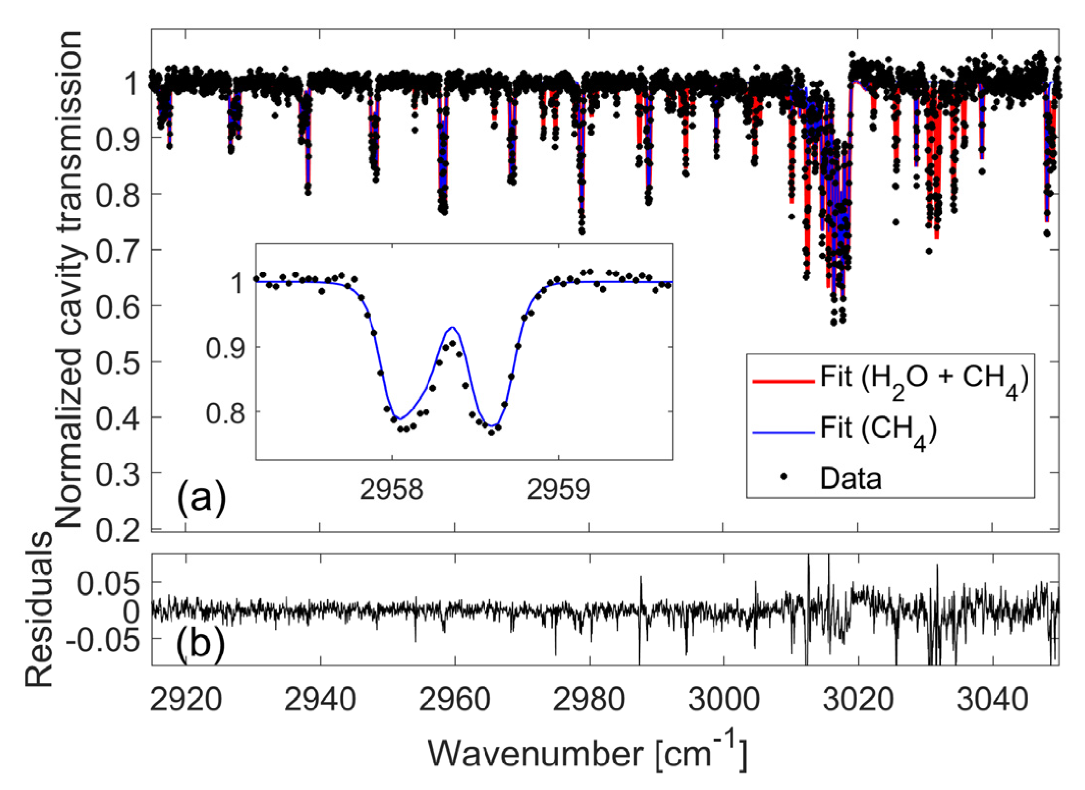
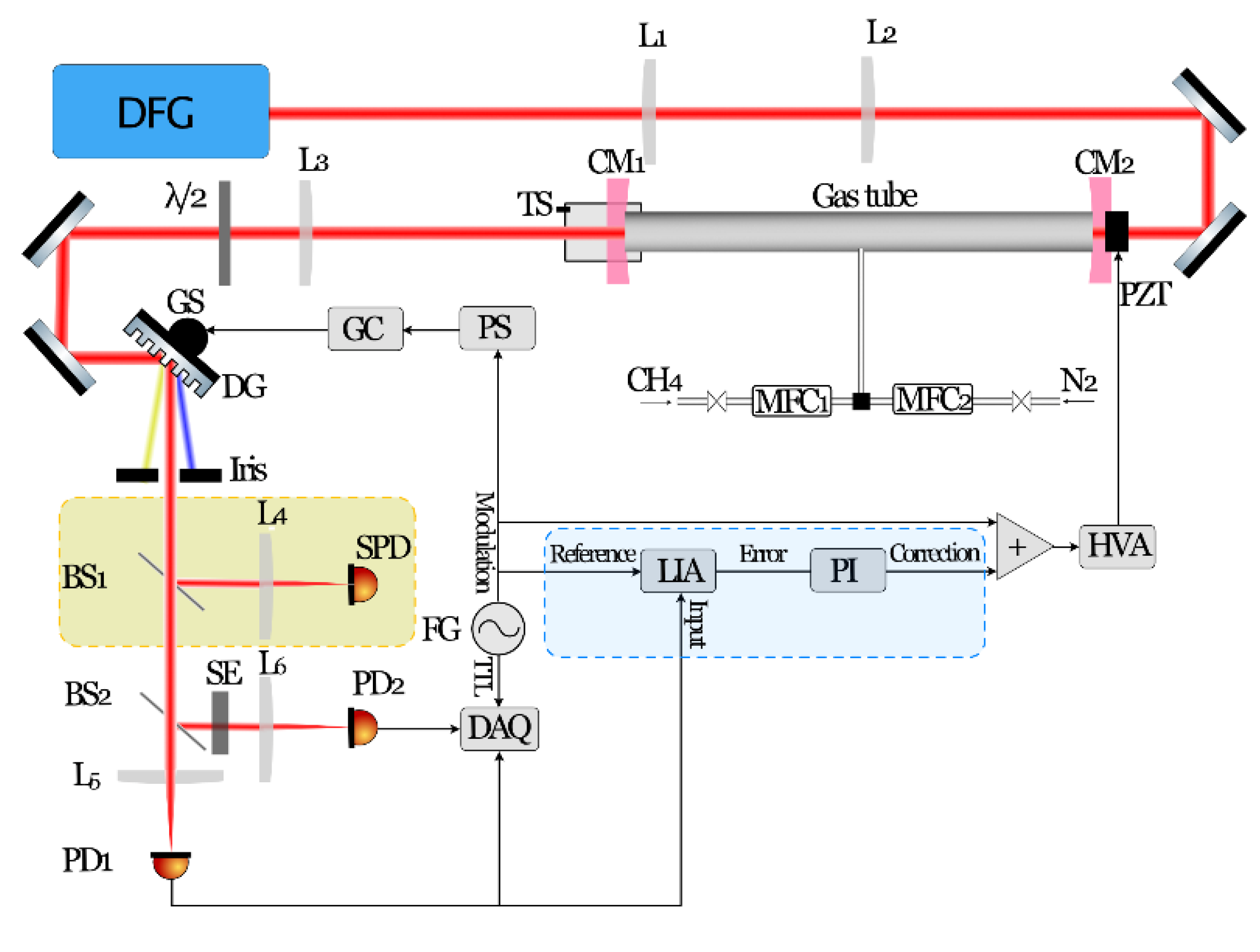
| This work MIR | Yb:fiber-pumped DFG 125 MHz | 3.7 THz @ 3.36 µm ΓV = 4.5 GHz | F = 430 FSR = 125 MHz | NEA = 6.1 × 10⁻⁷ cm−1 @ 50 ms FoM = 4.8 × 10⁻⁹ cm−1 Hz−1/2 | CH4 | Figure 5 |
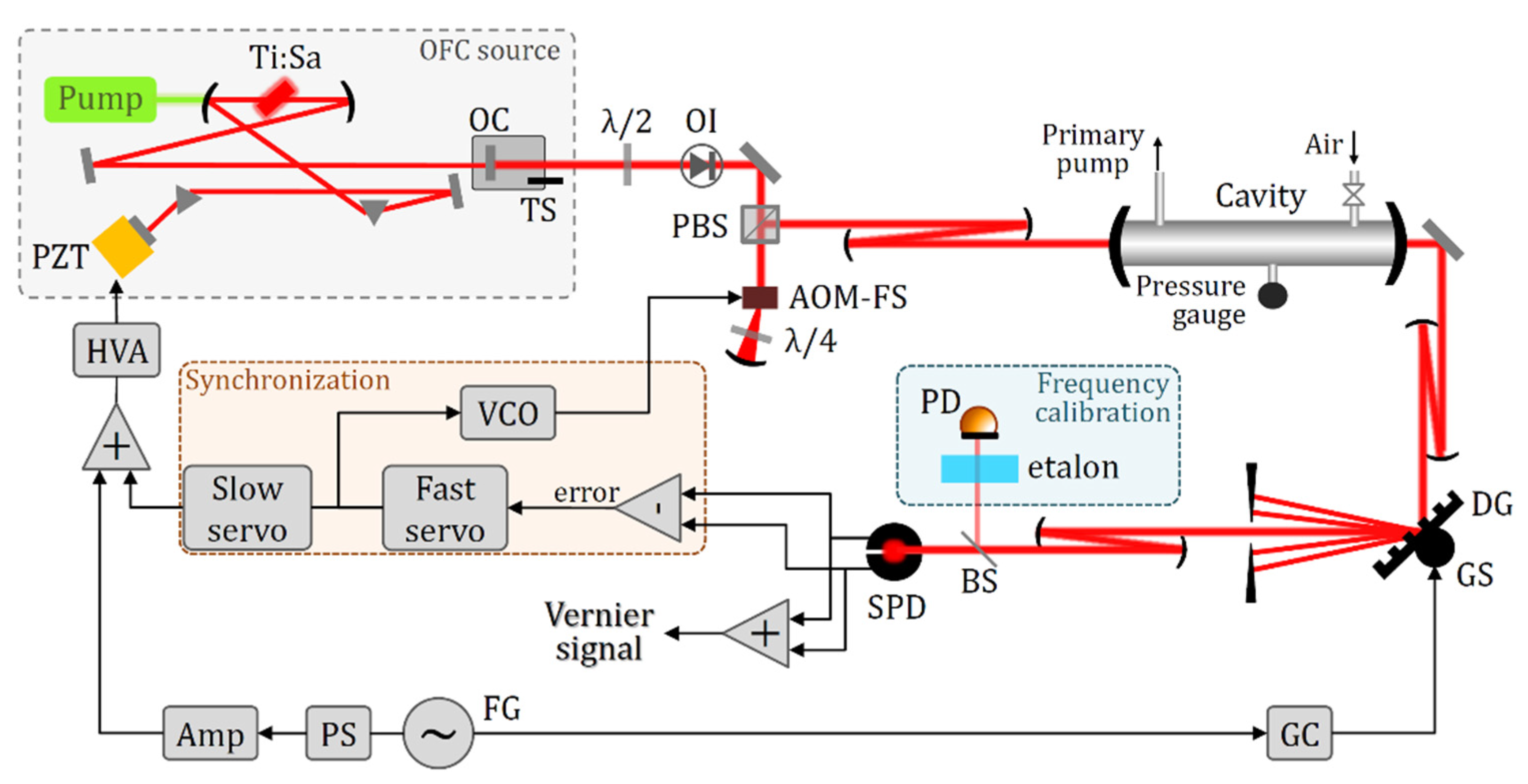
| This work NIR | Ti:sapphire 91 MHz | 3 THz @ 0.78 µm ΓV = 0.9 GHz | F = 16,400 FSR = 182 MHz | NEA = 4 × 10⁻¹⁰ cm−1 @ 1000 s FoM = 2.1 × 10⁻¹⁰ cm−1 Hz−1/2 | H2O in air | Figure 7 |
3.1. Comb-Resolved Vernier Spectroscopy
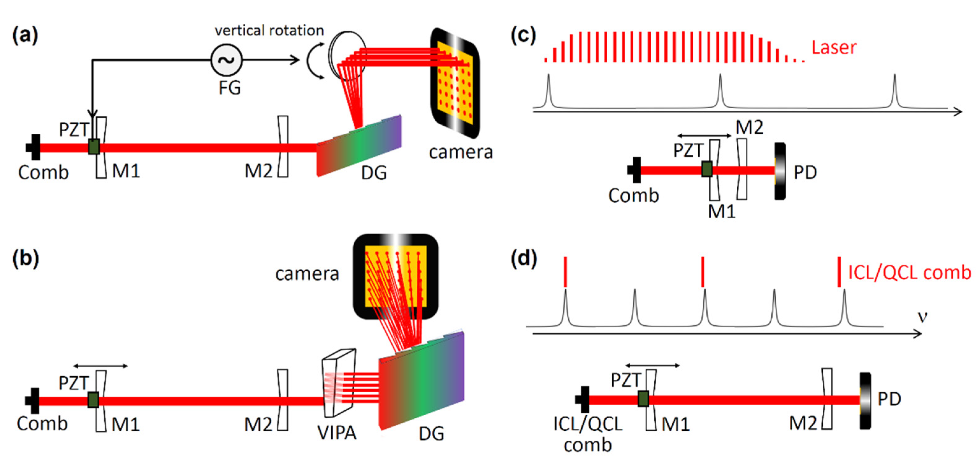
3.1.1. Grating-Based Vernier Spectrometers
3.1.2. Other Spectrometers Employing Vernier Filtering
3.1.3. Vernier Spectroscopy Based on Micro-Cavities or Chip-Scale Combs
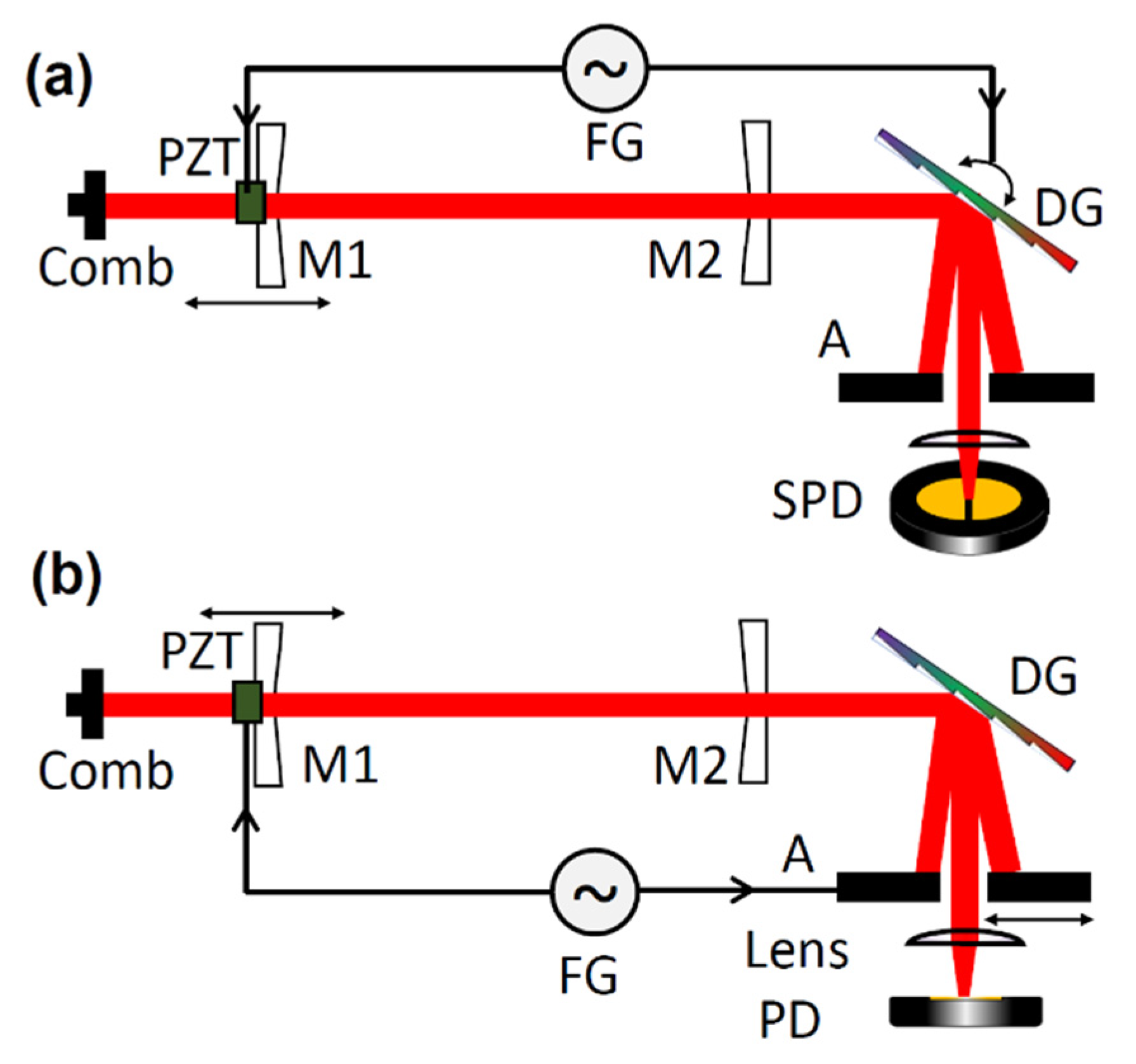
3.2. Continuous-Filtering Vernier Spectroscopy
3.3. Other Applications Employing Vernier Filtering
4. Mid-Infrared Continuous-Filtering Vernier Spectroscopy Based on a DFG Source
4.1. Experimental Setup
4.2. Procedures
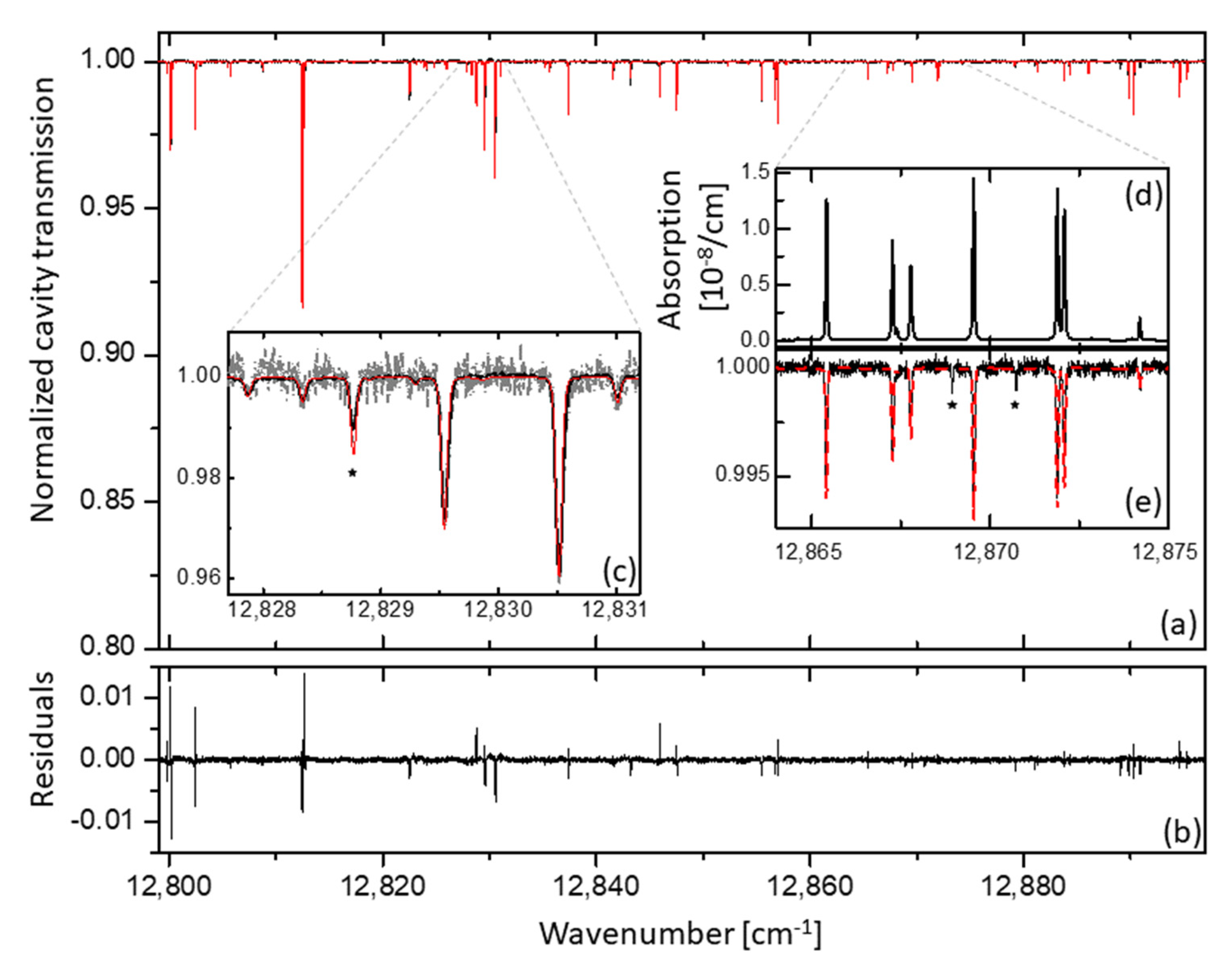
4.3. Results
5. Near-Infrared Continuous-Filtering Vernier Spectroscopy: High Sensitivity and Resolution Close to the Doppler Limit
5.1. Experimental Setup
5.2. Procedures
5.3. Results
6. Conclusions
Author Contributions
Funding
Institutional Review Board Statement
Informed Consent Statement
Data Availability Statement
Acknowledgments
Conflicts of Interest
References
- Gherman, T.; Romanini, D. Mode-locked cavity-enhanced absorption spectroscopy. Opt. Express 2002, 10, 1033–1042. [Google Scholar] [CrossRef] [PubMed] [Green Version]
- Diddams, S.A.; Hollberg, L.; Mbele, V. Molecular fingerprinting with the resolved modes of a femtosecond laser frequency comb. Nature 2007, 445, 627–630. [Google Scholar] [CrossRef] [PubMed]
- Mandon, J.; Guelachvili, G.; Picque, N. Fourier transform spectroscopy with a laser frequency comb. Nat. Photon. 2009, 3, 99–102. [Google Scholar] [CrossRef]
- Schiller, S. Spectrometry with frequency combs. Opt. Lett. 2002, 27, 766–768. [Google Scholar] [CrossRef] [PubMed] [Green Version]
- Thorpe, M.J.; Moll, K.D.; Jones, R.J.; Safdi, B.; Ye, J. Broadband cavity ringdown spectroscopy for sensitive and rapid molecular detection. Science 2006, 311, 1595–1599. [Google Scholar] [CrossRef] [Green Version]
- Bernhardt, B.; Ozawa, A.; Jacquet, P.; Jacquey, M.; Kobayashi, Y.; Udem, T.; Holzwarth, R.; Guelachvili, G.; Hansch, T.W.; Picque, N. Cavity-enhanced dual-comb spectroscopy. Nat. Photon. 2010, 4, 55–57. [Google Scholar] [CrossRef]
- Foltynowicz, A.; Ban, T.; Maslowski, P.; Adler, F.; Ye, J. Quantum-noise-limited optical frequency comb spectroscopy. Phys. Rev. Lett. 2011, 107, 233002. [Google Scholar] [CrossRef] [Green Version]
- Gohle, C.; Stein, B.; Schliesser, A.; Udem, T.; Hansch, T.W. Frequency comb Vernier spectroscopy for broadband, high-resolution, high-sensitivity absorption and dispersion spectra. Phys. Rev. Lett. 2007, 99, 263902. [Google Scholar] [CrossRef] [Green Version]
- Rutkowski, L.; Morville, J. Broadband cavity-enhanced molecular spectra from Vernier filtering of a complete frequency comb. Opt. Lett. 2014, 39, 6664–6667. [Google Scholar] [CrossRef]
- Thorpe, M.J.; Ye, J. Cavity-enhanced direct frequency comb spectroscopy. Appl. Phys. B 2008, 91, 397–414. [Google Scholar] [CrossRef] [Green Version]
- Kassi, S.; Didriche, K.; Lauzin, C.; Vaernewijckb, X.D.D.; Rizopoulos, A.; Herman, M. Demonstration of cavity enhanced FTIR spectroscopy using a femtosecond laser absorption source. Spectroc. Acta Part A Molec. Biomolec. Spectr. 2010, 75, 142–145. [Google Scholar] [CrossRef] [PubMed]
- Grilli, R.; Mejean, G.; Kassi, S.; Ventrillard, I.; Abd-Alrahman, C.; Romanini, D. Frequency comb based spectrometer for in situ and real time measurements of IO, BrO, NO2, and H2CO at pptv and ppqv levels. Environ. Sci. Technol. 2012, 46, 10704–10710. [Google Scholar] [CrossRef] [PubMed]
- Drever, R.W.P.; Hall, J.L.; Kowalski, F.V.; Hough, J.; Ford, G.M.; Munley, A.J.; Ward, H. Laser phase and frequency stabilization using an optical resonator. Appl. Phys. B 1983, 31, 97–105. [Google Scholar] [CrossRef]
- Foltynowicz, A.; Maslowski, P.; Fleisher, A.J.; Bjork, B.J.; Ye, J. Cavity-enhanced optical frequency comb spectroscopy in the mid-infrared application to trace detection of hydrogen peroxide. Appl. Phys. B 2013, 110, 163–175. [Google Scholar] [CrossRef] [Green Version]
- Siciliani de Cumis, M.; Eramo, R.; Coluccelli, N.; Cassinerio, M.; Galzerano, G.; Laporta, P.; De Natale, P.; Cancio Pastor, P. Tracing part-per-billion line shifts with direct-frequency-comb Vernier spectroscopy. Phys. Rev. A 2015, 91. [Google Scholar] [CrossRef]
- Kowzan, G.; Charczun, D.; Cygan, A.; Trawinski, R.S.; Lisak, D.; Maslowski, P. Broadband optical cavity mode measurements at Hz-Level precision with a comb-based VIPA spectrometer. Sci. Rep. 2019, 9, 1–10. [Google Scholar] [CrossRef] [PubMed]
- Vicentini, E.; Gambetta, A.; Coluccelli, N.; Wang, Y.; Laporta, P.; Galzerano, G. Direct-frequency-comb spectroscopy by a scanning Fabry-Pérot microcavity resonator. Phys. Rev. A 2020, 102, 033510. [Google Scholar] [CrossRef]
- Hébert, N.B.; Scholten, S.K.; White, R.T.; Genest, J.; Luiten, A.N.; Anstie, J.D. A quantitative mode-resolved frequency comb spectrometer. Opt. Express 2015, 23, 13991–14001. [Google Scholar] [CrossRef]
- Romanini, D.; Ventrillard, I.; Méjean, G.; Morville, J.; Kerstel, E. Introduction to cavity enhanced absorption spectroscopy. In Cavity-Enhanced Spectroscopy and Sensing; Gagliardi, G., Loock, H.-P., Eds.; Springer: Berlin, Germany, 2014. [Google Scholar]
- Rutkowski, L.; Morville, J. Continuous Vernier filtering of an optical frequency comb for broadband cavity-enhanced molecular spectroscopy. J. Quant. Spectr. Radiat. Transf. 2017, 187, 204–214. [Google Scholar] [CrossRef] [Green Version]
- Lu, C.; Senna Vieira, F.; Głuszek, A.; Silander, I.; Soboń, G.; Foltynowicz, A. Robust, fast and sensitive near-infrared continuous-filtering Vernier spectrometer. Opt. Express 2021, 29, 30155–30167. [Google Scholar] [CrossRef]
- Khodabakhsh, A.; Rutkowski, L.; Morville, J.; Foltynowicz, A. Mid-infrared continuous-filtering Vernier spectroscopy using a doubly resonant optical parametric oscillator. Appl. Phys. B 2017, 123, 1–12. [Google Scholar] [CrossRef]
- Zhu, F.; Bounds, J.; Bicer, A.; Strohaber, J.; Kolomenskii, A.A.; Gohle, C.; Amani, M.; Schuessler, H.A. Near-infrared frequency comb Vernier spectrometer for broadband trace gas detection. Opt. Express 2014, 22, 23026–23033. [Google Scholar] [CrossRef] [PubMed] [Green Version]
- Siciliani de Cumis, M.; Eramo, R.; Coluccelli, N.; Galzerano, G.; Laporta, P.; Cancio Pastor, P. Multiplexed direct-frequency-comb Vernier spectroscopy of carbon dioxide 2ν1 + ν3 ro-vibrational combination band. J. Chem. Phys. 2018, 148, 114303. [Google Scholar] [CrossRef]
- Siciliani de Cumis, M.; Eramo, R.; Jiang, J.; Fermann, M.E.; Cancio Pastor, P. Direct comb Vernier spectroscopy for fractional isotopic ratio determinations. Sensors 2021, 21, 5883. [Google Scholar] [CrossRef] [PubMed]
- Galli, I.; Bartalini, S.; Cancio, P.; Cappelli, F.; Giusfredi, G.; Mazzotti, D.; Akikusa, N.; Yamanishi, M.; De Natale, P. Mid-infrared frequency comb for broadband high precision and sensitivity molecular spectroscopy. Opt. Lett. 2014, 39, 5050–5053. [Google Scholar] [CrossRef] [PubMed]
- Coluccelli, N.; Cassinerio, M.; Redding, B.; Cao, H.; Laporta, P.; Galzerano, G. The optical frequency comb fibre spectrometer. Nat. Commun. 2016, 7, 1–11. [Google Scholar] [CrossRef]
- Gambetta, A.; Cassinerio, M.; Gatti, D.; Laporta, P.; Galzerano, G. Scanning micro-resonator direct-comb absolute spectroscopy. Sci. Rep. 2016, 6, 1–8. [Google Scholar] [CrossRef] [Green Version]
- Sterczewski, L.A.; Chen, T.-L.; Ober, D.C.; Markus, C.R.; Canedy, C.L.; Vurgaftman, I.; Frez, C.; Meyer, J.R.; Okumura, M.; Bagheri, M. Cavity-enhanced Vernier spectroscopy with a chip-scale mid-infrared frequency comb. arXiv 2021, arXiv:2112.03977. [Google Scholar] [CrossRef]
- Coddington, I.; Swann, W.C.; Newbury, N.R. Coherent dual-comb spectroscopy at high signal-to-noise ratio. Phys. Rev. A 2010, 82, 043817. [Google Scholar] [CrossRef] [Green Version]
- Khodabakhsh, A.; Ramaiah-Badarla, V.; Rutkowski, L.; Johansson, A.C.; Lee, K.F.; Jiang, J.; Mohr, C.; Fermann, M.E.; Foltynowicz, A. Fourier transform and Vernier spectroscopy using an optical frequency comb at 3–5.4 μm. Opt. Lett. 2016, 41, 2541–2544. [Google Scholar] [CrossRef]
- Lu, C.; Senna Vieira, F.; Schmidt, F.M.; Foltynowicz, A. Time-resolved continuous-filtering Vernier spectroscopy of H2O and OH radical in a flame. Opt. Express 2019, 27, 29521–29533. [Google Scholar] [CrossRef] [PubMed] [Green Version]
- Głuszek, A.; Senna Vieira, F.; Hudzikowski, A.; Wąż, A.; Sotor, J.; Foltynowicz, A.; Soboń, G. Compact mode-locked Er-doped fiber laser for broadband cavity-enhanced spectroscopy. Appl. Phys. B 2020, 126. [Google Scholar] [CrossRef]
- Western, C.M.; Carter-Blatchford, L.; Crozet, P.; Ross, A.J.; Morville, J.; Tokaryk, D.W. The spectrum of N2 from 4500 to 15,700 cm−1 revisited with PGOPHER. J. Quant. Spectr. Radiat. Transf. 2018, 219, 127–141. [Google Scholar] [CrossRef] [Green Version]
- Murphy, M.T.; Udem, T.; Holzwarth, R.; Sizmann, A.; Pasquini, L.; Araujo-Hauck, C.; Dekker, H.; D’Odorico, S.; Fischer, M.; Hansch, T.W.; et al. High-precision wavelength calibration of astronomical spectrographs with laser frequency combs. Mon. Not. R. Astron. Soc. 2007, 380, 839–847. [Google Scholar] [CrossRef]
- Li, C.H.; Benedick, A.J.; Fendel, P.; Glenday, A.G.; Kartner, F.X.; Phillips, D.F.; Sasselov, D.; Szentgyorgyi, A.; Walsworth, R.L. A laser frequency comb that enables radial velocity measurements with a precision of 1 cm s−1. Nature 2008, 452, 610–612. [Google Scholar] [CrossRef] [Green Version]
- Braje, D.A.; Kirchner, M.S.; Osterman, S.; Fortier, T.; Diddams, S.A. Astronomical spectrograph calibration with broad-spectrum frequency combs. Eur. Phys. J. D 2008, 48, 57–66. [Google Scholar] [CrossRef] [Green Version]
- McCracken, R.A.; Depagne, E.; Kuhn, R.B.; Erasmus, N.; Crause, L.A.; Reid, D.T. Wavelength calibration of a high resolution spectrograph with a partially stabilized 15-GHz astrocomb from 550 to 890 nm. Opt. Express 2017, 25, 6450–6460. [Google Scholar] [CrossRef]
- Ma, Y.X.; Meng, F.; Liu, Y.Z.; Zhao, F.; Zhao, G.; Wang, A.M.; Zhang, Z.G. Visible astro-comb filtered by a passively stabilized Fabry-Perot cavity. Rev. Sci. Instrum. 2019, 90, 013102. [Google Scholar] [CrossRef] [Green Version]
- Lešundák, A.; Voigt, D.; Cip, O.; van den Berg, S. High-accuracy long distance measurements with a mode-filtered frequency comb. Opt. Express 2017, 25, 32570–32580. [Google Scholar] [CrossRef] [Green Version]
- Xu, Z.W.; Shu, X.W. Fiber Optic Sensor Based on Vernier Microwave Frequency Comb. J. Light. Technol. 2019, 37, 3503–3509. [Google Scholar] [CrossRef]
- Zhang, L.; Lu, P.; Chen, L.; Huang, C.; Liu, D.; Jiang, S. Optical fiber strain sensor using fiber resonator based on frequency comb Vernier spectroscopy. Opt. Lett. 2012, 37, 2622–2624. [Google Scholar] [CrossRef]
- Hardy, B.; Raybaut, M.; Dherbecourt, J.B.; Melkonian, J.M.; Godard, A.; Mohamed, A.K.; Lefebvre, M. Vernier frequency sampling: A new tuning approach in spectroscopy—application to multi-wavelength integrated path DIAL. Appl. Phys. B 2012, 107, 643–647. [Google Scholar] [CrossRef]
- Soboń, G.; Martynkien, T.; Mergo, P.; Rutkowski, L.; Foltynowicz, A. High-power frequency comb source tunable from 2.7 to 4.2 μm based on difference frequency generation pumped by an Yb-doped fiber laser. Opt. Lett. 2017, 42, 1748–1751. [Google Scholar] [CrossRef]
- Sadiek, I.; Hjältén, A.; Senna Vieira, F.; Lu, C.; Stuhr, M.; Foltynowicz, A. Line positions and intensities of the ν4 band of methyl iodide using mid-infrared optical frequency comb Fourier transform spectroscopy. J. Quant. Spectr. Radiat. Transf. 2020, 255, 107263. [Google Scholar] [CrossRef]
- Silva de Oliveira, V.; Ruehl, A.; Masłowski, P.; Hartl, I. Intensity noise optimization of a mid-infrared frequency comb difference-frequency generation source. Opt. Lett. 2020, 45, 1914–1917. [Google Scholar] [CrossRef] [PubMed]
- Gordon, I.E.; Rothman, L.S.; Hill, C.; Kochanov, R.V.; Tan, Y.; Bernath, P.F.; Birk, M.; Boudon, V.; Campargue, A.; Chance, K.V.; et al. The HITRAN2016 molecular spectroscopic database. J. Quant. Spectr. Radiat. Transf. 2017, 203, 3–69. [Google Scholar] [CrossRef]
- Chang, C.-H.; Heilmann, R.K.; Schattenburg, M.L.; Glenn, P. Design of a double-pass shear mode acousto-optic modulator. Rev. Sci. Instrum. 2008, 79, 033104. [Google Scholar] [CrossRef] [PubMed]
- Vasilchenko, S.; Mikhailenko, S.N.; Campargue, A. Water vapor absorption in the region of the oxygen A-band near 760 nm. J. Quant. Spectr. Radiat. Transf. 2021, 275, 107847. [Google Scholar] [CrossRef]
- Hugi, A.; Villares, G.; Blaser, S.; Liu, H.C.; Faist, J. Mid-infrared frequency comb based on a quantum cascade laser. Nature 2012, 492, 229–233. [Google Scholar] [CrossRef]
- Timmers, H.; Kowligy, A.; Lind, A.; Cruz, F.C.; Nader, N.; Silfies, M.; Ycas, G.; Allison, T.K.; Schunemann, P.G.; Papp, S.B.; et al. Molecular fingerprinting with bright, broadband infrared frequency combs. Optica 2018, 5, 727–732. [Google Scholar] [CrossRef]
- Krzempek, K.; Tomaszewska, D.; Gluszek, A.; Martynkien, T.; Mergo, P.; Sotor, J.; Foltynowicz, A.; Sobon, G. Stabilized all-fiber source for generation of tunable broadband fCEO-free mid-IR frequency comb in the 7–9 μm range. Opt. Express 2019, 27, 37435–37445. [Google Scholar] [CrossRef]
- Krzempek, K.; Tomaszewska, D.; Foltynowicz, A.; Sobon, G. Fiber-based optical frequency comb at 3.3 μm for broadband spectroscopy of hydrocarbons Invited. Chin. Opt. Lett. 2021, 19, 08140. [Google Scholar] [CrossRef]


Publisher’s Note: MDPI stays neutral with regard to jurisdictional claims in published maps and institutional affiliations. |
© 2022 by the authors. Licensee MDPI, Basel, Switzerland. This article is an open access article distributed under the terms and conditions of the Creative Commons Attribution (CC BY) license (https://creativecommons.org/licenses/by/4.0/).
Share and Cite
Lu, C.; Morville, J.; Rutkowski, L.; Senna Vieira, F.; Foltynowicz, A. Cavity-Enhanced Frequency Comb Vernier Spectroscopy. Photonics 2022, 9, 222. https://doi.org/10.3390/photonics9040222
Lu C, Morville J, Rutkowski L, Senna Vieira F, Foltynowicz A. Cavity-Enhanced Frequency Comb Vernier Spectroscopy. Photonics. 2022; 9(4):222. https://doi.org/10.3390/photonics9040222
Chicago/Turabian StyleLu, Chuang, Jerome Morville, Lucile Rutkowski, Francisco Senna Vieira, and Aleksandra Foltynowicz. 2022. "Cavity-Enhanced Frequency Comb Vernier Spectroscopy" Photonics 9, no. 4: 222. https://doi.org/10.3390/photonics9040222
APA StyleLu, C., Morville, J., Rutkowski, L., Senna Vieira, F., & Foltynowicz, A. (2022). Cavity-Enhanced Frequency Comb Vernier Spectroscopy. Photonics, 9(4), 222. https://doi.org/10.3390/photonics9040222