sCMOS Noise-Corrected Superresolution Reconstruction Algorithm for Structured Illumination Microscopy

Abstract

Structured illumination microscopy (SIM) is widely applied due to its high temporal and spatial resolution imaging ability. sCMOS cameras are often used in SIM due to their superior sensitivity, resolution, field of view, and frame rates. However, the unique single-pixel-dependent readout noise of sCMOS cameras may lead to SIM reconstruction artefacts and affect the accuracy of subsequent statistical analysis. We first established a nonuniform sCMOS noise model to address this issue, which incorporates the single-pixel-dependent offset, gain, and variance based on the SIM imaging process. The simulation indicates that the sCMOS pixel-dependent readout noise causes artefacts in the reconstructed SIM superresolution (SR) image. Thus, we propose a novel sCMOS noise-corrected SIM reconstruction algorithm derived from the imaging model, which can effectively suppress the sCMOS noise-related reconstruction artefacts and improve the signal-to-noise ratio (SNR).

1. Introduction

Superresolution (SR) microscopy enables biological researchers to see nanoscale images of intracellular structures. Various SR fluorescence microscopy techniques, such as stimulated emission depletion (STED) [1,2,3], photoactivated localization microscopy (PALM) [4,5,6], stochastic optical reconstruction microscopy (STORM) [7,8,9], and structured illumination microscopy (SIM) [10,11,12,13,14,15], have come to the fore during the past 20 years. These SR technologies can break the optical diffraction limit and achieve a spatial resolution of approximately 20~100 nm compared to the ~200 nm of conventional microscopes. SR SIM has a relatively high temporal resolution and long-term imaging ability and is a promising SR imaging technique for live-cell imaging [16,17,18].

Although an electron-multiplying charge-coupled device (EMCCD) can detect signals with sufficient SNR and sensitivity for SR SIM, its readout speed is slow and it has small sensor areas [19]. Therefore, scientific-grade complementary metal-oxide-semiconductor (sCMOS) cameras are a better choice for offering sufficient quantum efficiency and much faster readout speed, significantly increasing the data acquisition rate and improving the temporal resolution [20,21,22]. With the sCMOS camera, Hessian-SIM was developed to increase the temporal resolution and image rapidly moving vesicles or loops in the endoplasmic reticulum with a temporal resolution of 188 Hz [23].

Generally, images captured from sCOMS contain two kinds of typical noises: shot noise and readout noise. For the former, which comes from the arrival of photons at the camera sensor and is a stochastic process, we usually constitute shot noise following Poisson counting statistics. Shot noise equals the square root of the input signal and is always present due to its physical essence. For the latter, the readout noise comes from nonuniform pixel characteristics due to the process variation in the on-pixel amplifier circuitry and column-based readout structures [20]. This results in unique sCMOS pixel-dependent noise, which negatively impacts the image reconstruction and creates single-molecule localization errors in PALM/STORM and artefacts in SIM reconstruction. To correct the pixel-independent readout noise in the raw images, Huang et al. proposed a simplified sCMOS noise model incorporating single-pixel-dependent offset, gain, and variance. They developed a noise-corrected SMSN reconstruction algorithm [24] and a noise-correction algorithm for an sCMOS camera for a broad spectrum of microscopes [25]. By combining camera physics and sparsely layered filtering, Biagio et al. proposed a content-adaptive algorithm to automatically correct sCMOS-relatedd noise (ACsN) for fluorescence microscopy, which reduces the most relevant noise sources in the sCMOS camera while preserving the fine details of the signal [26]. Xue et al. developed a Hessian-based SMLM (Hessian-SMLM) method to correct the single-pixel variance, gain, and offset and effectively eliminated the pixel-dependent readout noise, especially under conditions of low signal-to-noise ratios [27]. Lin et al. presented a nonuniform noise model of sCMOS cameras that incorporates pixel-specific read-noise, offset, and sensitivity variation. Thus, they developed a new weighted least squared (WLS) fitting method designed to remove the heterogeneity of sCMOS pixels [20]. Li et al. developed the photon transfer curve (PTC) method to fully assess the performance of low-light cameras, including the sCMOS camera [28].

Despite all of these correction algorithms developed for the sCMOS cameras, correcting artefacts due to heterogeneous pixel noise in SIM reconstruction remains unexplored. However, the different offset and variance in each pixel causes artefacts in reconstructed SIM images (especially in hot pixels). To minimize these artefacts caused by readout noise, we propose an sCMOS noise model based on SIM imaging and present a novel noise-corrected algorithm for SIM reconstruction. The reconstruction is conducted in the spatial domain based on the stable bi-conjugate gradients descent algorithm (Bi-CGSTAB) [29] and split Bergman algorithm (SB) [30]. In all simulation experiments, the algorithm can effectively suppress the sCMOS pixel-dependent readout noise-related reconstruction artefacts, improve the SNR, and slightly increase the contrast of the reconstructed SR image using various regularized constraints.

2. Methods

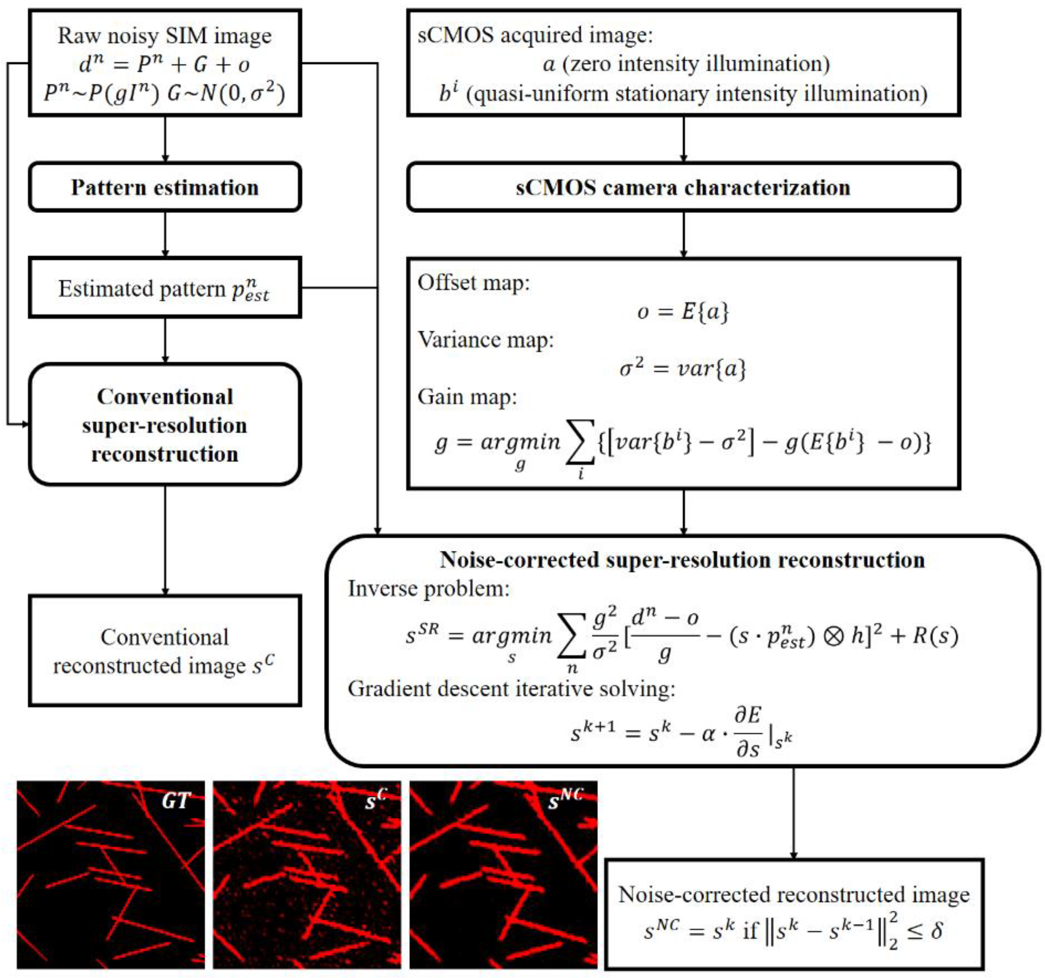
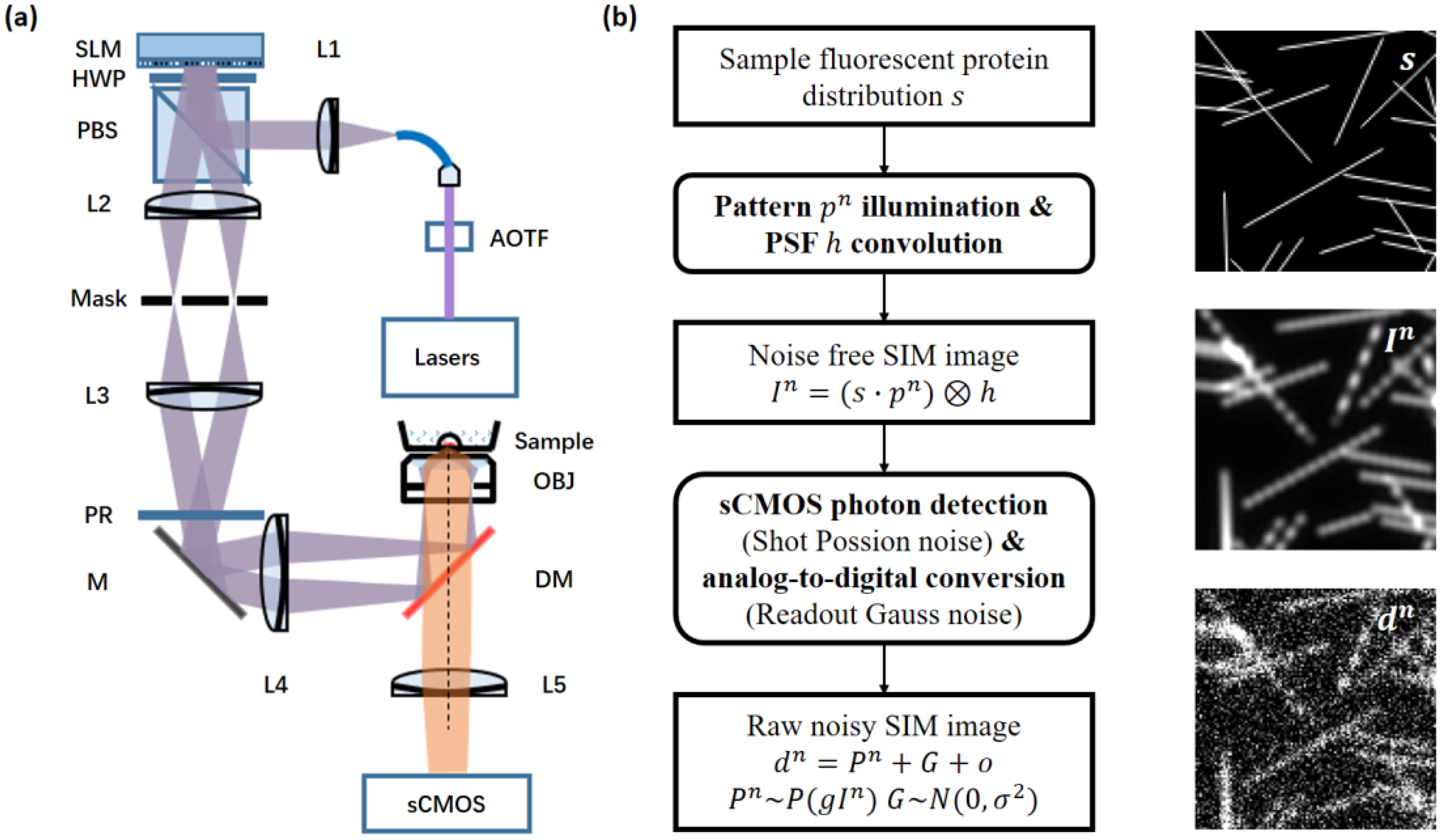
2.1. SIM Imaging Model

Compared to conventional wide-field fluorescence microscopy, SIM can double the spatial resolution by illuminating the observed sample with pattern illumination generated by the interference of two beams of light (Figure 1a). Without considering noise, the fluorescence emission distribution $I^n$ detected by the camera can be expressed as:

$$I^n({\overrightarrow{r}}_k)=[s({\overrightarrow{r}}_l)\cdot p^n({\overrightarrow{r}}_l)]\otimes h({\overrightarrow{r}}_k-{\overrightarrow{r}}_l),$$

(1)

where ${\overrightarrow{r}}_l$ and ${\overrightarrow{r}}_k$ are the spatial coordinate vectors of the sample and camera, respectively, $s\left({\overrightarrow{r}}_l\right)$ is the fluorophore spatial distribution in the sample, $p^n\left({\overrightarrow{r}}_l\right)$ is the intensity distribution according to the illumination pattern sequence $n$, $h\left({\overrightarrow{r}}_k-{\overrightarrow{r}}_l\right)$ is the point spread function, and $\otimes$ represents the convolutional operation. The model can be discretized and expressed as:

$$I_k^n={\displaystyle \sum }_l{s}_l{p}_l^n{h}_{kl}$$

(2)

where $l$ and $k$ are the discrete spatial coordinates as substitutes for the continuous spatial coordinate vectors ${\overrightarrow{r}}_l$ and ${\overrightarrow{r}}_k$.

2.2. sCMOS Camera Noise Model

In SIM imaging, the acquired raw image contains noise from the camera. sCMOS camera noise primarily consists of shot noise and readout noise. While shot noise stems from the photon detection process, readout noise originates from the electronics built around the detector chip [24]. When photons are detected on the sensor chip, the camera’s analogue-to-digital unit (ADU) count output follows a probability distribution described here by the convolution of a Poisson distribution and a Gaussian distribution. The Poisson distribution represents the shot noise of photon detection, and the Gaussian distribution results from the readout noise (Figure 1b). Then, the pixel-dependent conditional probability density function (PDF) of the sCMOS camera can be expressed as:

$$P\left(d_k^n|I_k^n\right)=A{\displaystyle \sum }_{q_k^n=0}^{\infty }\frac{1}{q_k^n}{e}^{-I_k^n}{\left(I_k^n\right)}^{q_k^n}\frac{1}{\sqrt{2\pi }{\sigma }_k}{e}^{-\frac{{\left(d_k^n-g_k{q}_k^n-o_k\right)}^2}{2{\sigma }_k^2}}$$

(3)

where $d_k^n$ is the specific counts obtained by the sCMOS in the kth pixel when the sample is illuminated by the nth pattern (in units of $\mathrm{ADU}$). $A$ is the normalization constant, $q_k^n$ is the number of fluorescence photoelectrons as a random variable (in units of $e^{-}$), and $I_k^n$ is the number of expected fluorescence photoelectrons (in units of $e^{-}$) and defined by Equation (2), ${\sigma }_k^2$ is the readout noise variance in the kth pixel (in units of ${\mathrm{ADU}}^2$), $g_k$ is the amplification gain of the kth pixel (in units of $\mathrm{ADU}/e^{-}$), and $o_k$ is the readout noise mean (offset) of the kth pixel (in units of $\mathrm{ADU}$).

For the convenience of later deduction, the distribution of random variables $d_k^n$ can be equivalently expressed as:

$$d_k^n=P_k^n+G_k+o_k$$

(4)

where random variable $P_k^n$ follows the Poisson distribution with mean value and variance value equal to $g_k{I}_k^n$:

$$P_k^n~P\left(g_k{I}_k^n\right)$$

(5)

Random variable $G_k$ follows the Gaussian distribution with mean value equal to zero and variance value equal to ${\sigma }_k^2$:

$$G_k~N\left(0,{\sigma }_k^2\right)$$

(6)

Due to the noise, pixels on sCMOS cameras appear to flicker even when there are no expected incident photons. This noise level changes drastically across pixels from 1~2 ${\mathrm{ADU}}^2$ to 1000~2000 ${\mathrm{ADU}}^2$ [25]. This noise drastically reduces the image SNR and makes quantitative analysis a challenge.

2.3. sCMOS Camera Characterization

To characterize the readout noise of the sCMOS camera, the offset, gain, and variance values need to be measured (Figure 2). The offset value describes a constant level of ADUs pre-engineered into the readout process to prevent negative ADUs caused by the readout noise [24]. After acquiring a series of images in an environment with zero expected incident photons, the offset value $o_k$ and the variance value ${\sigma }_k^2$ of the kth sCMOS pixel can be calculated as:

$$o_k=\frac{1}{M}{\displaystyle \sum }_{m=1}^M{a}_k^m$$

(7)

$${\sigma }_k^2=\frac{1}{M}{\displaystyle \sum }_{m=1}^M{\left(a_k^m\right)}^2-{\left(\frac{1}{M}{\displaystyle \sum }_{m=1}^M{a}_k^m\right)}^2$$

(8)

where $a_k^m$ is the ADU count at the mth frame for the kth pixel and $M$ is the total number of dark frames acquired.

By illuminating the camera with quasi-uniform stationary intensity patterns and recording a series of image sequences at different average intensity levels, the gain value $g_k$ of the kth sCMOS pixel can be calculated as:

$$g_k=\underset{g}{argmin}{\displaystyle \sum _i\left\{\left[{\left({\sigma }_k^i\right)}^2-{\sigma }_k^2\right]-g\left(o_k^i-o_k\right)\right\}}$$

(9)

where:

$$o_k^i=\frac{1}{M_i}{\displaystyle \sum }_{m=1}^{M_i}{b}_k^{im}$$

(10)

The variance value ${\left({\sigma }_k^i\right)}^2$ can be defined as:

$${\left({\sigma }_k^i\right)}^2=\frac{1}{M_i}{\displaystyle \sum }_{m=1}^{M_i}{\left(b_k^{im}\right)}^2-{\left(\frac{1}{M_i}{\displaystyle \sum }_{m=1}^{M_i}{b}_k^{im}\right)}^2$$

(11)

where $b_k^{im}$ is the ADU count at the ith illuminating intensity and the mth frame for the kth pixel, and $M_i$ is the total frame number acquired at the ith illuminating intensity.

2.4. sCMOS Noise-Corrected SIM Reconstruction Algorithm

Based on the deduction in Section 2.2., a new random variable $Z_k^n$ can be defined and expressed as:

$$Z_k^n=\frac{d_k^n-o_k}{g_k}+\frac{{\sigma }_k^2}{g_k^2}$$

(12)

The mean value of the Gaussian distribution equals its variance value. When the mean of a Poisson distribution is large, it becomes similar to a Gaussian distribution. Then, the distribution of random variable $Z_k^n$ approximately follows the Gaussian distribution and can be expressed as:

$$Z_k^n~N\left(\frac{{\sigma }_k^2}{g_k^2}+I_k^n,\frac{{\sigma }_k^2}{g_k^2}+I_k^n\right)$$

(13)

For simplification, the $I_k^n$ term in the variance value of $Z_k^n$ is ignored, and then the approximate CPDF of $Z_k^n$ can be expressed as:

$$P\left(Z_k^n|I_k^n\right)=\frac{g_k}{\sqrt{2\pi }{\sigma }_k}{e}^{-\frac{{\left(g_k^2{Z}_k^n-g_k^2{I}_k^n-{\sigma }_k^2\right)}^2}{2g_k^2{\sigma }_k^2}}$$

(14)

The approximate CPDF of $d_k^n$ can be calculated by substituting $Z_k^n$ into Equation (14) with Equation (12) and expressed as:

$$P\left(d_k^n|I_k^n\right)=\frac{g_k}{\sqrt{2\pi }{\sigma }_k}{e}^{-\frac{{\left(d_k^n-g_k{I}_k^n-o_k\right)}^2}{2{\sigma }_k^2}}$$

(15)

The sample fluorophore spatial distribution $s$ is determined by maximizing the posterior probability $P\left(s|d\right)$ defined as:

$$P\left(s|d\right)={\displaystyle \prod }_n{\displaystyle \prod }_{k}P\left(s|d_k^n\right)$$

(16)

where $P\left(s|d_k^n\right)$ can be calculated with Bayes’ rule and expressed as:

$$P\left(s|d_k^n\right)=\frac{P(d_k^n|s)P\left(s\right)}{P\left(d_k^n\right)}\propto P(d_k^n|s)$$

(17)

For operational convenience, the merit function $E\left(s\right)$ is defined as the logarithm of $P\left(s|d\right)$ and calculated by combining Equations (2) and (15)–(17). The simplified form of $E\left(s\right)$ can be expressed as:

$$E\left(s\right)={\displaystyle \sum _n{\displaystyle \sum _k\left[\frac{g_k^2}{{\sigma }_k^2}{\left(\frac{d_k^n-o_k}{g_k}-{\displaystyle \sum }_l{s}_l{p}_l^n{h}_{kl}\right)}^2\right]}}$$

(18)

The regularization constraint can assist optimization convergence and prevent overfitting. The Tikhonov regularization term $R_T\left(s\right)$, high-frequency suppression regularization term $R_{HP}\left(s\right)$, and nonnegativity regularization term $R_{NN}\left(s\right)$ are appended to the merit function, and the whole constrained optimization problem can be expressed as:

$$\underset{s}{min}{\displaystyle \sum _n{\displaystyle \sum _k\left[\frac{g_k^2}{{\sigma }_k^2}{\left(\frac{d_k^n-o_k}{g_k}-{\displaystyle \sum }_l{s}_l{p}_l^n{h}_{kl}\right)}^2\right]}}+\alpha R_T\left(s\right)+\beta R_{HP}\left(s\right)+R_{NN}\left(s\right)$$

(19)

where $\alpha$ and $\beta$ are the weights of the corresponding regularization terms, and the definition of each regularization term can be expressed as:

$$R_T\left(s\right)={\displaystyle \sum }_{l}w{s}_l^2$$

(20)

$$R_{HP}\left(s\right)={\displaystyle \sum }_k{\left({\displaystyle \sum }_l{s}_l{h}_{kl}^{hp}\right)}^2$$

(21)

$$R_{NN}\left(s\right)=\prod \left(s\ge 0\right)$$

(22)

where $w$ is the parameter of the Tikhonov regularization term and $h^{hp}$ is the parameter of the high-frequency suppression regularization term as a tunable high-pass filter. The matriculated representation of Equation (19) can be expressed as:

$$\underset{s}{min}{\displaystyle \sum }_n\Vert A_{n}s-b_n{\Vert }_2^2+\alpha s^{T}Cs+\beta s^T{D}^{T}Ds+\prod \left(s\ge 0\right)$$

(23)

where $s$ is the fluorophore spatial distribution in the sample as a column vector, $A_n$ is the illumination by the nth pattern and PSF convolution operation as a matrix, $b_n$ is the image obtained by the sCMOS as a column vector, $C$ and $D$ are the Tikhonov parameter matrix and high-pass filter matrix, respectively, and ${[\cdot ]}^T$ represents the conjugate transpose operation.

The constrained optimization problem defined by Equation (23) can be solved by the combination of the stable bi-conjugate gradients descent algorithm (Bi-CGSTAB) and the split Bergman algorithm (SB). The Bi-CGSTAB algorithm can minimize convex differentiable functional such as the L2-functional in Equation (23) and avoid severe cancellation effects caused by the irregular convergence behavior of the conventional gradients’ descent algorithm [29]. The SB algorithm allows for the minimization of convex nondifferentiable functional efficiency and leads to a solution update for which L2-functional and the nonnegativity functions are decoupled and solved separately [30]. Using the Bergman method, the equivalent formulation of Equation (23) can be expressed as:

$$\begin{gathered} (s^{k+1},v^{k+1})=\underset{s,v}{argmin}{\displaystyle \sum }_n\Vert A_{n}s-b_n^k{\Vert }_2^2+\delta \Vert s-v+{\mu }_v^k{\Vert }_2^2+\alpha s^{T}Cs+\beta s^T{D}^{T}Ds+\prod \left(v\ge 0\right) \\ {b}_n^{k+1}=b_n^k+b_n-A_n{s}^{k+1} \\ {\mu }_v^{k+1}={\mu }_v^k+s^{k+1}-v^{k+1} \end{gathered}$$

(24)

with $b_n^0=b_n$, $s^0=0$, $v^0=0$. The variables $s^{k+1}$ and $v^{k+1}$ can be solved separately due to the decoupled relationship between them:

$$s^{k+1}=\underset{s}{argmin}{\displaystyle \sum }_n\Vert A_{n}s-b_n^k{\Vert }_2^2+\delta \Vert s-v^k+{\mu }_v^k{\Vert }_2^2+\alpha s^{T}Cs+\beta s^T{D}^{T}Ds$$

(25)

$$v^{k+1}=\underset{v}{argmin}\delta \Vert s^{k+1}-v+{\mu }_v^k{\Vert }_2^2+\prod \left(v\ge 0\right)$$

(26)

The elements of $v^{k+1}$ in Equation (26) are solved independently using a shrinkage formula due to the decoupled relationship between them:

$$v^{k+1}=max\left(s^{k+1}+{\mu }_v^k,0\right)$$

(27)

To solve the variable $s^{k+1}$ in Equation (25) with the Bi-CGSTAB algorithm, the merit function can be expanded as:

$$\underset{s}{argmin}{s}^{T}Ms-s^{T}n+p$$

(28)

where $M$ is a matrix, $n$ is a column vector, and $p$ is a scalar and can be calculated as:

$$M={\displaystyle \sum }_n{A}_n^T{A}_n+\delta I+\alpha C+\beta D^{T}D$$

(29)

$$n={\displaystyle \sum }_n{A}_n^T{b}_n^k+\delta \left(v^k-{\mu }_v^k\right)$$

(30)

$$p={\displaystyle \sum }_n\left\{-{\left(b_n^k\right)}^T{A}_{n}s+\delta {\left(b_n^k\right)}^T{b}_n^k\left[{\left({\mu }_v^k\right)}^T-{\left(v^k\right)}^T\right]\left(s-v^k+{\mu }_v^k\right)\right\}$$

(31)

where $I$ is the unit matrix. According to convex optimization theory, the solution $\widehat{s}$ of Equation (28) satisfies the following equation:

$$M\widehat{s}=n$$

(32)

which can be solved by the Bi-CGSTAB algorithm (Algorithm 1).

Algorithm 1. Pseudocode of the Bi-CGSTAB algorithm.

Bi-CGSTAB algorithm

Input: $M$, $n$ Initialization: $s^0=0$, $r^0=n-M{s}^0$, ${\widehat{r}}^0=r^0$, ${\rho }^0={\omega }^0=\alpha =1$,$v^0=p^0=0$ Iteration: For $k=1,2,3\cdots$  ${\rho }^k=\left({\widehat{r}}^0,r^{k-1}\right)$,$\beta =\left(\alpha {\rho }^k\right)/\left({\rho }^{k-1}{\omega }^{k-1}\right)$ $p^k=r^{k-1}+\beta \left(p^{k-1}-{\omega }^{k-1}{v}^{k-1}\right)$ $v^k=M{p}^k$ $\alpha ={\rho }^k/\left({\widehat{r}}^0,v^k\right)$ $b=r^{k-1}-\alpha v^k$ $t=Mb$ ${\omega }^k=\left(t,b\right)/\left(t,t\right)$ $s^k=s^{k-1}+\alpha p^k+{\omega }^{k}b$ if $\Vert s^k-s^{k-1}{\Vert }_2^2\le \delta$ Terminating. Else $r^k=b-{\omega }^{k}t$ End Output:$s=s^k$

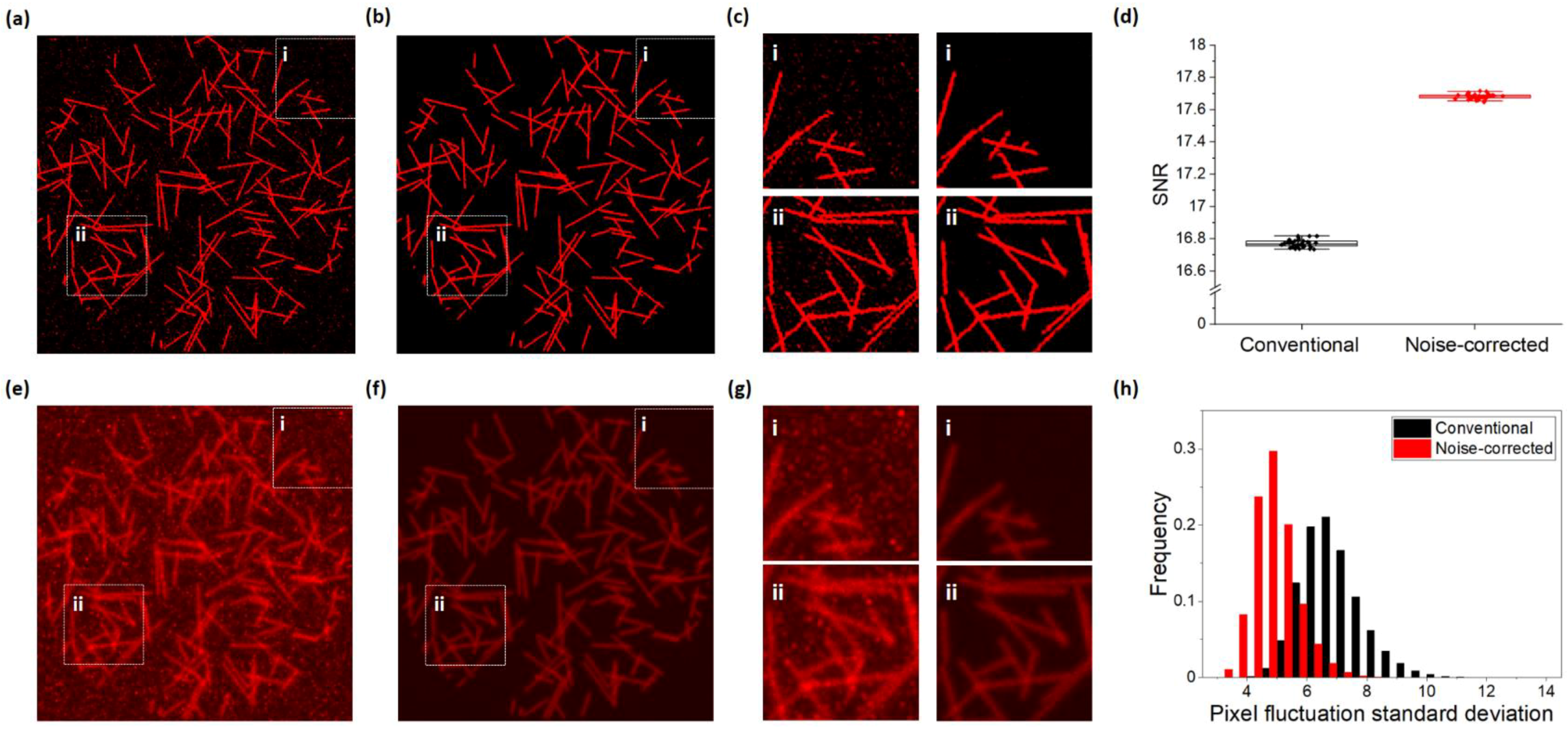
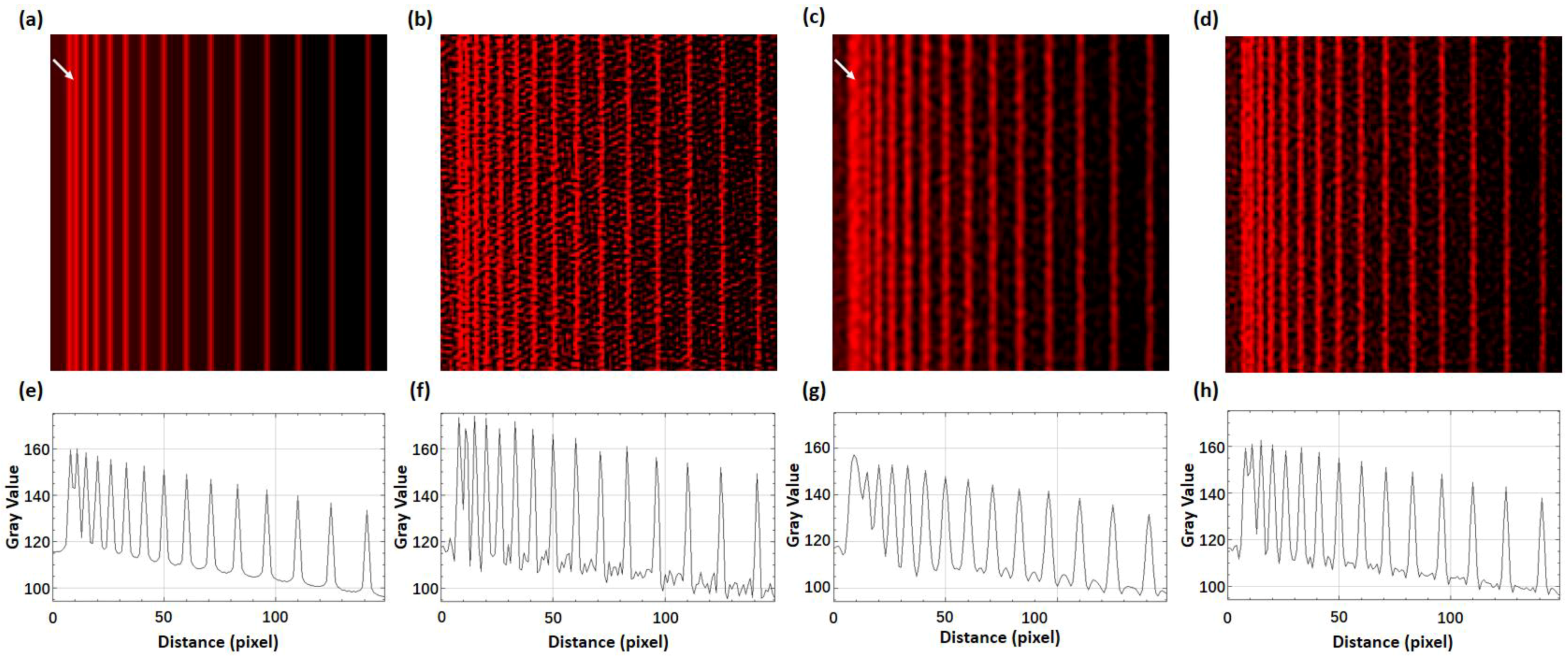
3. Results

Compared with the conventional Wiener algorithm, and not considering the sCMOS noise, our proposed sCMOS noise-corrected SIM reconstruction algorithm can suppress the sCMOS noise-related spatial punctiform artefact in the SR reconstructed image, especially in the background area (Figure 3a–c). The punctiform artefact within the SR image reconstructed by the conventional algorithm is widely distributed (Figure 3a) and can be observed within the zoomed-in image (left in Figure 3c). After the proposed sCMOS noise-correction algorithm, the punctiform artefact is eliminated globally (Figure 3b) and invisible to human eyes (right in Figure 3c). The statistical box plot (Figure 3d) shows that the SNR of the SR image reconstructed by the conventional algorithm is ~16.8 and improved to ~17.7 by the proposed sCMOS noise-corrected SIM reconstruction algorithm, which is consistent with the phenomenon of punctiform artefact elimination above.

Furthermore, the intensity fluctuation standard deviation in each pixel over time, which reflects the temporal pixel fluctuation map, is shown in Figure 3e–g. The bright and punctiform structures within the temporal pixel fluctuation map corresponding to the conventional algorithm (Figure 3e and left in Figure 3g) indicate that the intensity fluctuation standard deviation of the corresponding pixels is relatively large. That is, the temporal fluctuation noise level of these pixels is relatively high. These structures reflecting high noise levels almost completely disappear (Figure 3f, and right in Figure 3g) with the proposed sCMOS noise-corrected SIM reconstruction algorithm. Hence, the temporal fluctuation noise is suppressed effectively. The statistical histogram of the temporal pixel fluctuation map (Figure 3h) confirms the conclusion above. The pixel intensity fluctuation standard deviation distribution corresponding to the conventional algorithm moves left globally after the sCMOS noise correction. The mode interval of the pixel intensity fluctuation standard deviation corresponding to the noise-corrected algorithm is ~4.75, which is 30% lower than the ~6.75 of the conventional algorithm.

The punctiform artefact and high pixel intensity fluctuation standard deviation may result in negative impacts on the data analysis. For example, the dynamic analysis of the organelle structures and functions in the living cell is likely to be misleading when the sCMOS noise-related pixel intensity fluctuation is severe in the SR reconstructed images. Such possible mistakes can be avoided by the proposed sCMOS noise-corrected SIM reconstruction algorithm.

To further verify the robustness of our method, we validated our approach with different SNRs. We found that the SNR of the SR image reconstructed by the proposed algorithm is robust under various shot noise and readout noise levels (

Table 1. SNR of the SR reconstructed image under various noise levels.

Shot Noise Level	Readout Noise Level	SNR
		Conventional	Noise-Corrected
100	10	11.167	13.349
	20	10.336	12.942
	30	9.627	12.521
150	10	12.280	14.338
	20	11.432	13.865
	30	10.852	13.496
200	10	11.149	13.363
	20	8.734	10.562
	30	5.294	6.460

). The average improvement percentage of the SNR is ~22%, and the maximum improvement percentage of the SNR is ~30% when the shot noise level and the readout noise level are equal to 100 and 30, respectively. The robustness of the proposed algorithm guarantees broad applicability in the reconstruction of the raw data at various noise levels. The simulated ground truth image is identical to Figure 3. The shot noise level is quantified by the parameter representing the total photon count of each emitter on the simulated samples. The read out noise level is quantified by the parameter multiplied to the variance map of the sCMOS camera. For example, if the read out noise level is set as L, the variance of the ith pixel in the sCMOS camera variance map is V. Then, the variance of Gauss noise is added to the ith pixel is set as LV when we generate the simulation SIM raw noisy data. For all of the reconstructions, only the Tikhonov regularized constraint is used and the regularized term weight parameter $\alpha$ is set as 2.

The proposed algorithm can also combine regularization to further suppress the noise. The SR images reconstructed by the noise-corrected SIM reconstruction algorithm with nonnegativity, high-frequency suppression, and Tikhonov regularized constraint are compared in Figure 4.

The ground truth image contains the chirped line structure (Figure 4a). The shot noise level and read out noise level of SIM raw data are 150 and 10, respectively. Within all of the reconstructed SR images (Figure 4b–d), the reconstruction with a nonnegativity regularized constraint exhibits the highest contrast (Figure 4b). The grey value range of the profile corresponding to the nonnegativity regularized constraint is from ~96 to ~174 (Figure 4f), which is ~30% and ~16% wider than the high-frequency suppression regularized constraint (Figure 4g) and Tikhonov regularized constraint (Figure 4h). However, the reconstruction with the nonnegativity regularized constraint still produces severe artefacts. Thus, the nonnegativity regularized constraint is usually not used alone as denoising regularization in the reconstruction of low SNR raw images.

In contrast, the reconstruction of the high-frequency suppression regularized constraint has the lowest artefact level compared with those of the other two methods (Figure 4c). The smoothness of profiles provides additional evidence of artefact suppression (Figure 4g). However, the two lines are indistinguishable in reconstructing the high-frequency suppression method (Figure 4c, white arrow), which means the resolution decreased for reconstructing the high-frequency suppression regularized constraint. In addition, the average full width at half maximum (FWHM) of the ten spikes on the right of the profile corresponding to the high-frequency suppression regularized constraint (Figure 4g) is ~3 pixels, which is ~33% larger than the ground truth profile (Figure 4e).

The resolution, artefact level, and contrast level of the SR image reconstructed with Tikhonov regularization (Figure 4d) are the most moderate within all three reconstructed SR images (Figure 4b–d). Additionally, the profile is also the closest to the ground truth profile (Figure 4e,h). Therefore, the Tikhonov regularized constraint is a more general choice than the nonnegativity regularized constraint and high-frequency suppression regularized constraint.

4. Discussion

Although quite a few sCMOS noise-correction algorithms for various imaging technologies have been developed, the sCMOS noise-correction algorithm in SIM reconstruction has never been presented to date as far as we know. The experiment shows that the proposed sCMOS noise-corrected SIM reconstruction algorithm can suppress the sCMOS readout noise-related spatial punctiform artefact and temporal fluctuation noise caused in the SR reconstructed images and improve the SNR by 22%, which is validated by the simulation experiments.

We combined the proposed sCMOS noise-corrected reconstruction with three regular terms. The combination with the nonnegativity regularized constraint can be suitable for raw data with a relatively high SNR, while the combination with high-frequency suppression regularization is more appropriate for raw data with a low SNR. As the most general method, the sCMOS noise-corrected SIM reconstruction algorithm with Tikhonov regularization provides the most moderate reconstructed SR images in terms of the resolution, artefact level, and contrast level.

5. Conclusions

A nonuniform sCMOS noise model in the SIM imaging process is established and a novel sCMOS noise-corrected SIM reconstruction algorithm is proposed based on the imaging noise model. The sCMOS noise causes artefacts in the reconstructed SR image and the novel algorithm can effectively suppress the artefacts and improve the SNR.

References

- Hell, S.; Wichmann, J. Breaking the Diffraction Resolution Limit by Stimulated-Emission: Stimulated-Emission-Depletion Fluorescence Microscopy. Opt. Lett. 1994, 19, 780–782. [Google Scholar] [CrossRef] [PubMed]
- Dyba, M.; Jakobs, S.; Hell, S. Immunofluorescence stimulated emission depletion microscopy. Nat. Biotechnol. 2003, 21, 1303–1304. [Google Scholar] [CrossRef] [PubMed]
- Gao, P.; Prunsche, B.; Zhou, L.; Nienhaus, K.; Nienhaus, G.U. Background suppression in fluorescence nanoscopy with stimulated emission double depletion. Nat. Photonics 2017, 11, 163–169. [Google Scholar] [CrossRef]
- Betzig, E.; Patterson, G.H.; Sougrat, R.; Lindwasser, O.W.; Olenych, S.; Bonifacino, J.S.; Davidson, M.W.; Lippincott-Schwartz, J.; Hess, H.F. Imaging Intracellular Fluorescent Proteins at Nanometer Resolution. Science 2006, 313, 1642–1645. [Google Scholar] [CrossRef] [PubMed] [Green Version]
- Hess, S.T.; Girirajan, T.P.K.; Mason, M.D. Ultra-high resolution imaging by fluorescence photoactivation localization microscopy. Biophys. J. 2006, 91, 4258–4272. [Google Scholar] [CrossRef] [PubMed] [Green Version]
- Errico, C.; Pierre, J.; Pezet, S.; Desailly, Y.; Lenkei, Z.; Couture, O.; Tanter, M. Ultrafast ultrasound localization microscopy for deep super-resolution vascular imaging. Nature 2015, 527, 499–502. [Google Scholar] [CrossRef]
- Huang, B.; Wang, W.; Bates, M.; Zhuang, X. Three-dimensional super-resolution imaging by stochastic optical reconstruction microscopy. Science 2008, 319, 810–813. [Google Scholar] [CrossRef] [Green Version]
- Linde, S.; Löschberger, A.; Klein, T.; Heidbreder, M.; Wolter, S.; Heilemann, M.; Sauer, M. Direct stochastic optical reconstruction microscopy with standard fluorescent probes. Nat. Protoc. 2011, 6, 991–1009. [Google Scholar] [CrossRef]
- Rust, M.J.; Bates, M.; Zhuang, X. Sub-diffraction-limit imaging by stochastic optical reconstruction microscopy (STORM). Nat. Methods 2006, 3, 793–795. [Google Scholar] [CrossRef] [Green Version]
- Gustafsson, M.G.L. Surpassing the lateral resolution limit by a factor of two using structured illumination microscopy. Short Commun. J. Microsc. 2000, 198, 82–87. [Google Scholar] [CrossRef] [Green Version]
- Cragg, G.E.; So, P. Lateral resolution enhancement with standing evanescent waves. Opt. Lett. 2000, 25, 46–48. [Google Scholar] [CrossRef] [PubMed]
- Frohn, J.T.; Knapp, H.F.; Stemmer, A. True optical resolution beyond the Rayleigh limit achieved by standing wave illumination. Proc. Natl. Acad. Sci. USA 2000, 97, 7232–7236. [Google Scholar] [CrossRef] [PubMed] [Green Version]
- Günther, B.; Hehn, L.; Jud, C.; Hipp, A.; Dierolf, M.; Pfeiffer, F. Full-field structured-illumination super-resolution X-ray transmission microscopy. Nat. Commun. 2019, 10, 2494. [Google Scholar] [CrossRef] [PubMed] [Green Version]
- York, A.; Parekh, S.; Nogare, D.; Fischer, R.; Temprine, K.; Mione, M.; Chitnis, A.; Combs, C.; Shroff, H. Resolution doubling in live, multicellular organisms via multifocal structured illumination microscopy. Nat. Methods 2012, 9, 749–754. [Google Scholar] [CrossRef]
- Mudry, E.; Belkebir, K.; Girard, J.; Savatier, J.; Le Moal, E.; Nicoletti, C.; Allain, M.; Sentenac, A. Structured illumination microscopy using unknown speckle patterns. Nat. Photonics 2012, 6, 312–315. [Google Scholar] [CrossRef]
- Kner, P.; Chhun, B.B.; Griffis, E.R.; Winoto, L.; Gustafsson, M.G.L. Super-resolution video microscopy of live cells by structured illumination. Nat. Methods 2009, 6, 339–342. [Google Scholar] [CrossRef] [Green Version]
- Shao, L.; Kner, P.; Rego, E.H.; Gustafsson, M.G.L. Super-resolution 3D microscopy of live whole cells using structured illumination. Nat. Methods 2011, 12, 1044–1046. [Google Scholar] [CrossRef]
- Fiolka, R.; Shao, L.; Rego, E.H.; Davidson, M.W.; Gustafsson, M.G.L. Time-lapse two-color 3D imaging of live cells with doubled resolution using structured illumination. Proc. Natl. Acad. Sci. USA 2012, 109, 5311–5315. [Google Scholar] [CrossRef] [Green Version]
- Diekmann, R.; Till, K.; Müller, M.; Simonis, M.; Schüttpelz, M.; Huser, T. Characterization of an industry-grade CMOS camera well suited for single molecule localization microscopy-high performance super-resolution at low cost. Sci. Rep. 2017, 7, 14425. [Google Scholar] [CrossRef]
- Lin, R.; Clowsley, A.H.; Jayasinghe, I.D.; Baddeley, D.; Soeller, C. Algorithmic corrections for localization microscopy with sCMOS cameras-characterisation of a computationally efficient localization approach. Opt. Express 2017, 25, 11701–11716. [Google Scholar] [CrossRef] [Green Version]
- Zhang, Z.; Wang, Y.; Piestun, R.; Huang, Z. Characterizing and correcting camera noise in back-illuminated sCMOS cameras. Opt. Express 2021, 29, 6668–6690. [Google Scholar] [CrossRef] [PubMed]
- Saurabh, S.; Maji, S.; Bruchez, M.P. Evaluation of sCMOS cameras for detection and localization of single Cy5 molecules. Opt. Express 2012, 20, 7338–7349. [Google Scholar] [CrossRef] [PubMed]
- Huang, X.; Fan, J.; Li, L.; Liu, H.; Wu, R.; Wu, Y.; Wei, L.; Mao, H.; Lal, A.; Xi, P.; et al. Fast, long-term, super-resolution imaging with Hessian structured illumination microscopy. Nat. Biotechnol. 2018, 36, 451–459. [Google Scholar] [CrossRef] [PubMed]
- Huang, F.; Hartwich, T.; Rivera-Molina, F.; Lin, Y.; Duim, W.; Long, J.; Uchil, P.; Myers, J.; Baird, M.; Mothes, W.; et al. Video-rate nanoscopy using sCMOS camera-specific single-molecule localization algorithms. Nat. Methods 2013, 10, 653–658. [Google Scholar] [CrossRef]
- Liu, S.; Mlodzianoski, M.; Hu, Z.; Ren, Y.; McElmurry, K.; Suter, D.; Huang, F. sCMOS noise-correction algorithm for microscopy images. Nat. Methods 2017, 14, 760–761. [Google Scholar] [CrossRef]
- Mandracchia, B.; Hua, X.; Guo, C.; Son, J.; Urner, T.; Jia, S. Fast and accurate sCMOS noise correction for fluorescence microscopy. Nat. Commun. 2020, 11, 94. [Google Scholar] [CrossRef] [Green Version]
- Xue, F.; He, W.; Xu, F.; Zhang, M.; Chen, L.; Xu, P. Hessian single-molecule localization microscopy using sCMOS camera. Biophys. Rep. 2018, 4, 215–221. [Google Scholar] [CrossRef]
- Li, L.; Li, M.; Zhang, Z.; Huang, Z. Assessing low-light cameras with photon transfer curve method. J. Innov. Opt. Health Sci. 2016, 9, 1630008. [Google Scholar] [CrossRef] [Green Version]
- van der Vorst, H.A. Bi-CGSTAB: A Fast and Smoothly Converging Variant of Bi-CG for the Solution of Nonsymmetric Linear Systems. Siam J. Sci. Stat. Comput. 1992, 13, 631–644. [Google Scholar] [CrossRef]
- Abascal, P.; Chamorro-Servent, J.; Aguirre, J. Fluorescence diffuse optical tomography using the split Bregman method. Med. Phys. 2011, 38, 6275–6284. [Google Scholar] [CrossRef] [Green Version]