Article

Density Awareness and Neighborhood Attention for LiDAR-Based 3D Object Detection

College of Intelligence Science and Technology, National University of Defence Technology, Changsha 410073, China
*
Author to whom correspondence should be addressed.
Photonics 2022, 9(11), 820; https://doi.org/10.3390/photonics9110820
Submission received: 19 September 2022 / Revised: 14 October 2022 / Accepted: 21 October 2022 / Published: 2 November 2022
(This article belongs to the Special Issue Photonic Application in the Automotive Industry)

Abstract

:
Light detection and ranging (LiDAR) is widely used in the automotive industry as it can provide point cloud information containing precise distances. Three-dimensional (3D) object detection based on LiDAR point clouds is significant for environment perception tasks. However, feature learning for point clouds remains challenging. This paper proposes a two-stage voxel-based LiDAR 3D object detector, referred to as density-aware and neighborhood attention (DenNet), that focuses on the neighborhood information of objects. DenNet mainly integrates two modules: voxel density-aware (VDA) and neighborhood attention (NA). VDA introduces density information of the point cloud. Here, point cloud density information was added as voxel features in the voxel-based framework to alleviate the information loss during voxelization. Additionally, to extract neighbor information, the characteristics of 3D objects were analyzed for traffic scenes. The NA mechanism was adopted, which localizes the receptive field for each query to its nearest neighboring points. DenNet yielded competitive results, as compared with state-of-the-art methods, for the KITTI and One Million Scenes (ONCE) datasets; notably, it afforded an improvement of 3.96% relative to the baseline mean average precision on the more challenging ONCE dataset.

1. Introduction

Driven by the rapid developments in the intelligent vehicle industry over recent years, various advanced photonic sensors have been deployed on vehicles to meet the growing demands for environmental perception in the intelligent automotive industry. Among these, light detection and ranging (LiDAR) sensors provide more accurate distance information and are more useful under various adverse conditions, including darkness and backlight, as compared with passive sensors such as cameras. These sensors are widely used in lane line detection, urban scene segmentation, simultaneous localization and mapping, and object detection. Three-dimensional (3D) object detection based on LiDAR is another essential task; its main function entails using the point cloud information obtained via LiDAR to classify other traffic participants in surrounding environments, such as cars and pedestrians, and yield accurate 3D boxes [1]. It provides the basic perception information for a series of downstream tasks such as path planning and driving following. Unlike object detection in the image domain, 3D object detection affords 3D prediction frames. This detection frame can be expressed using Equation (1):
B = x c , y c , z c , l , w , h , θ ,   class  
where ( x c , y c , z c ) represents the center coordinate of a 3D box; l , w , h are the length, width, and height of a cuboid on the ground, respectively; θ is the heading angle; and class denotes the category of the 3D object.
Furthermore, unlike the uniform and regular pixels in 2D images, point cloud data are sparse, unstructured, and disordered [2]. Thus, extracting features from point cloud data has remained an extremely challenging task. Even widely used backbone networks such as VGG and ResNet cannot be directly employed for 3D point cloud data. Therefore, point- and grid-based methods have emerged as possible solutions for processing. Point-based methods use the point cloud feature network represented by PointNet to learn the original point cloud information through downsampling and feature learning. Alternatively, grid-based methods use the idea of image detection and divide the point cloud data into uniform grids before processing. The mainstream division methods include pillars and voxels. Voxels are 3D cubes that comprise certain points; the points in each cube are then averaged and used as the feature of each voxel and input into the subsequent feature extraction backbone network. Pillars can be considered as special voxels, wherein the voxel size is unlimited along the vertical direction; this highlights their main advantage. Because the vehicles do not overlap when driving normally, we divide the point cloud data evenly according to equal-sized columns in the 3D space and extract the point cloud features in the columns to generate a bird’s-eye view (BEV) feature map. The mature image detection can then be used for processing. Owing to the high efficiency and ease of computation, this is a mature detector used for intelligent driving applications. However, because of the significant quantization loss, the upper limit of the accuracy for the pillar-based method remains low. Hence, a voxel-based algorithm was adopted in this current study.
Based on a comparison of the object detection results on the image with the detection results on the point clouds, as shown in Figure 1, three important pieces of knowledge are noted: (1) In the image, the detection frames may overlap; however, in a 3D space, there will be no overlap among the objects. Due to the imaging characteristics of LIDAR, there will be some occlusion, which is also clearly shown in the red circle in the right picture in Figure 1. Except for some special cases such as the moment passengers exit a car, the detection bounding boxes and the objects on the BEV map will not overlap. (2) There is no significant semantic correlation between two different cars. In the typical self-attention operation, the global feature weight for a certain area is considered. However, in the autopilot scene, vehicles moving in the opposite direction of the road are not explicitly related to the vehicles in this lane. Therefore, it is not ideal to blindly extract global attention; instead, the main focus should be on the perception of vehicles and their surroundings. (3) There exists a significant difference in the density of the point clouds situated at short and long distances; a significant difference is also noted in the density features between the vehicle and the ground, which are clustered for target recognition and semantic segmentation in traditional machine learning. Considering this analysis, we plan to improve the voxel-based method based on the density characteristics and neighborhood information of the objects.
Density is based on the basic principle that the closer the object is to the LiDAR, the higher the density is. Based on this principle, there are several other flexible forms. For instance, the density at the edge of the object is often lower than that at the center, and the density of an occluded object is less than that of an object that is not occluded. Existing methods utilizing point cloud density information mainly focus on the sampling and region-of-interest (ROI) optimization parts.
Some point-based detectors [3,4] use density information during the process of point cloud downsampling, because point clouds with high densities occupy a large proportion in a limited dataset if they are uniformly sampled, while the distant sparse point cloud that needs to be sampled cannot be collected in sufficient quantities. Therefore, it is beneficial to use the density to adjust the sampling of point clouds. Point cloud density information also plays an important role for small objects. Compared to cars, objects such as pedestrians tend to have a smaller reflective area and an irregular distribution. PDV [5] uses the correlation among the density information to optimize the detection frame for the ROI stage. It is often used in existing voxelization-based methods to adaptively adjust the ROI receptive field as supplementary information in the ROI stage. In this paper, we believe that the density information can directly reflect the state of the object, such as distance and occlusion. However, the existing voxel feature extraction (VFE) algorithms ignore the density information. The voxel features obtained in the previous steps do not contain density features, and this can be regarded as a significant loss of information.
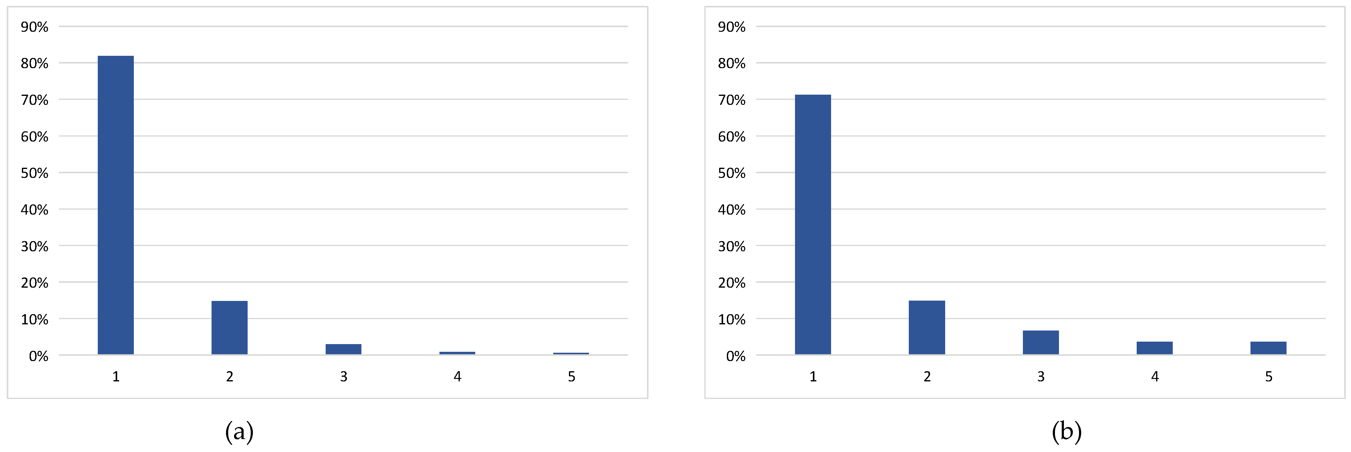
Based on a thorough investigation and analysis of the data in the KITTI [6] and ONCE [7] datasets, as shown in Figure 2, under the general setting, the voxel size was set as (0.1 m, 0.1 m, 0.15 m) for KITTI and (0.1 m, 0.1 m, 0.2 m) for ONCE, the voxels without points which are named as empty are not included in the statistics. The number of points in most voxels is 1 and 2, indicating a typical long-tailed distribution. Using the number of points in each voxel as a feature of the voxel will not result in an obvious increase in the volume of information. Therefore, we refer to the multi-scale calculation method and interactively calculate the point cloud of a single voxel and the surrounding point cloud to obtain the density feature and add it to the voxel.
In the 2D backbone stage, we add the neighborhood attention (NA) [8] module, which is based on improvements in existing transformers for point cloud applications. Currently, there are several challenges associated with the application of transformers on point clouds, including computational complexity and additional data for training. Analyzing the reality of 3D objects in traffic scenes reveals that there is no overlap of the object detection frames in the point cloud space and no strong correlation between a single object and another object. Hence, blindly applying the global information will not afford a significant change. Instead, this may result in an increase in the computational cost and subsequently have an adverse impact on the detector. Thus, we apply the NA mechanism, which localizes the receptive field for each token to its neighborhood. This helps improve the accuracy of the regression of the object bounding box. We also add the coordinate attention (CA) module to improve convolutional feature representation.
The novelty and contributions of this work can be summarized as follows:
  • This work summarizes the use of density information in existing 3D object detectors and proposes DenNet, which focuses on the density and neighbor information of 3D objects.
  • Voxel density-aware (VDA) is proposed to retain the density information during voxelization. We also introduce NA and CA to the 2D backbone network to efficiently enrich the token representations with fine-level information.
  • In this manner, we achieved competitive performance for the KITTI dataset, especially in the cyclist category, where we realized state-of-the-art (SOTA) results. On the more complex ONCE dataset, which conforms with the Chinese traffic environment, we achieved an improvement of 3.96% relative to the baseline mAP.

2. Related Works

2.1. Voxel-Based 3D Object Detection

Unlike images, 3D point clouds are disordered and scattered across a 3D space. A potential approach to handle such 3D point clouds is the voxelization of point clouds into regular 3D voxels. The voxel-based 3D object detector was first proposed by Zhou et al. [9], and its approach for extracting voxel point cloud features using VFE has been widely integrated into subsequent studies. Yan et al. [10] proposed SECOND, which is a milestone for voxel-based methods; under this approach, sparse convolution makes the heavy 3D convolution feasible in theoretical and practical applications. Deng et al. [11] proposed Voxel R-CNN, whereby they broke the traditional perception that the accuracy of voxelization is inferior to that of point-based detectors owing to the loss of information caused by the voxelization of point clouds. They demonstrated that by using their process, the detection accuracy can be improved significantly. Compared with the PV R-CNN proposed by Shi et al. [12], its operating efficiency is also improved considerably. Moreover, Mao et al. [13] proposed VOTR, which was the first voxel-like detector to incorporate transformers into a 3D backbone; notably, this was a successful start for the next step to introduce transformer-like algorithms, which were highly successful in the image and natural language processing (NLP) domains. Generally, the accuracy of voxel-based detectors is lower than that of point-based detectors, mainly because of the inherent voxel quantization errors. This work is based on Voxel R-CNN, which is computationally efficient and performs well on the KITTI dataset.

2.2. Point Density Estimation

Mao et al. [14] proposed the density-aware radius prediction module, which can adapt to different point density levels by dynamically adjusting the focusing range of the ROIs. PDV is then used for second-stage optimization by locating voxel features using point centroids, and ROI grid pooling is included as an additional feature to encode local point densities. Further, kernel density estimation is used to encode the local voxel feature density at each grid point ball query, and subsequently, a novel point density location encoding is employed for self-attention between the grid points coding. Starting from the classical approach, Gao et al. [15] proposed a dynamic clustering algorithm in order to accommodate the spatial inhomogeneity of the point cloud distribution. The algorithm uses elliptic functions to describe the neighborhood and dynamically adjusts the semi-minor and semi-major of the nearest neighbors according to the location of the core points. Ning et al. [4] proposed DA-3DSSD, which was a point-based detector. By introducing density information, a density-aware factor was added to the sampling process, and the density weight was introduced into the process of sampling the farthest point. This helped improve the detection of sparse objects by retaining additional foreground points. Compared with the aforementioned studies, in this work, we directly added the density information in the voxelization process, which afforded a good foundation for high-quality proposals in a single stage.

2.3. Transformers for 3D Object Detection

Transformer models such as encoder–decoder architectures have become the most widely adopted algorithms in NLP. They have been integrated into computer vision as well, owing to their ability to model long-range dependencies. As a type of irregular variable-length data, 3D point cloud data are more suitable for the transformer, and thus, they have attracted significant attention worldwide. Sheng et al. [16] proposed a two-stage detector called CT3D, which was based on channel transformation, to improve 3D object detection performance. The input to the channel transformer originated from the region proposal network. Further, a channel-wise decoding module was used to enrich the query–key interactions through channel-wise reweighting, which effectively incorporated multi-level contexts. Mao et al. [13] further introduced VOTR, which was the first transformer-based backbone for 3D object detection. They proposed a submanifold voxel module and a sparse voxel module to extract features from non-empty and empty voxels, respectively. Fan et al. [17] also proposed SST, which adopted a pure transformer structure and replaced the stride with a single stride. Driven by its local attention mechanism and ability to handle sparse data, the detector could overcome receptive field shrinkage under the single-stride setting and also prevent heavy computational overheads. The proposed NA module is based on the neighborhood attention transformer that was proposed by Hassani et al. [8], which is an efficient, accurate, and scalable hierarchical transformer.

3. Methods

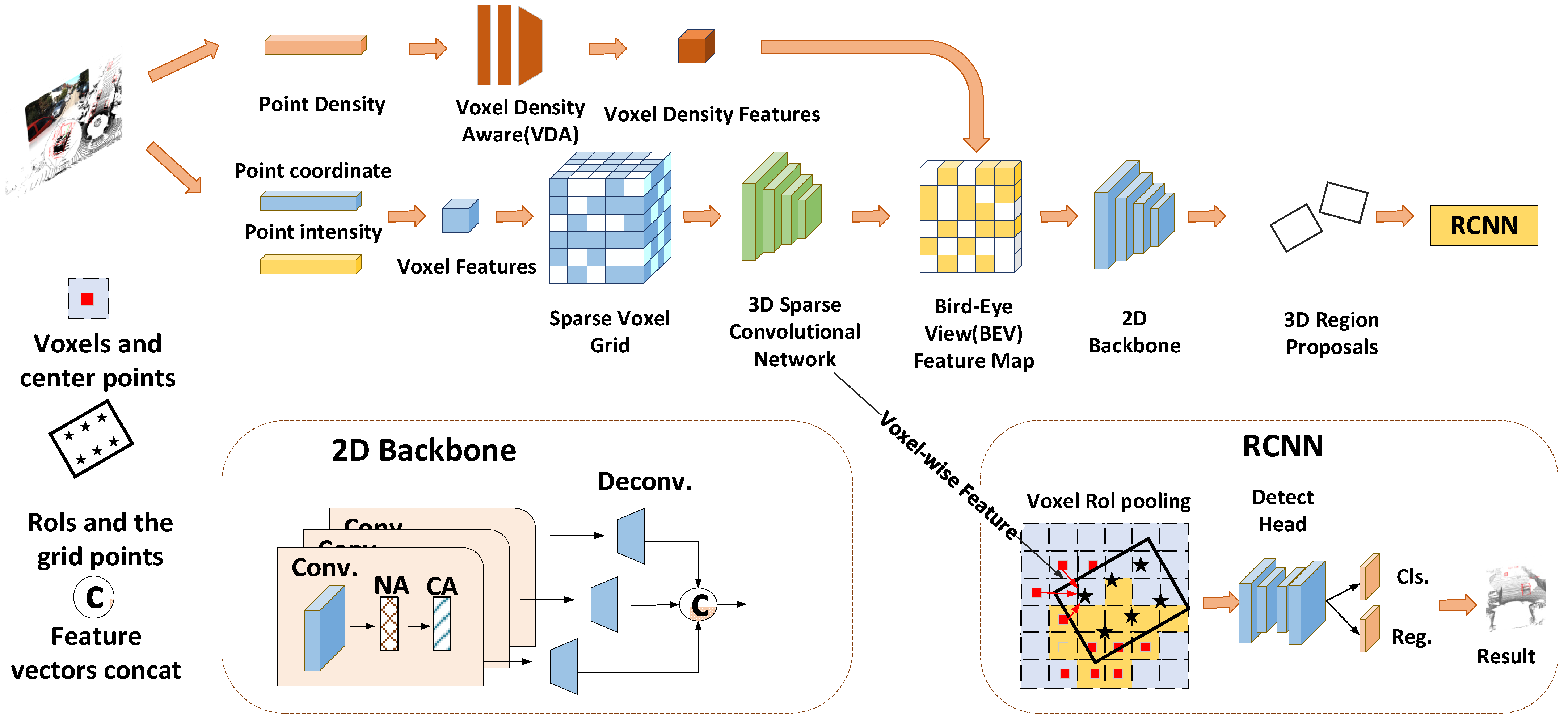
As shown in Figure 3, a VDA module was added to the original Voxel R-CNN with the aim of extracting voxel density features. Further, the multi-scale NA module and coordinate attention (CA) module were added to the 2D backbone to deal with BEV maps. We introduce these two modules separately in the following sections.

3.1. Revisiting Voxel R-CNN Backbone

The baseline of the proposed approach is the Voxel R-CNN, which is a voxel-based detector. Many existing high-performance 3D detectors are point-based because their structure helps in preserving precise spatial information better. However, point-wise features incur high computational overheads because of the unstructured storage. By contrast, the voxel-based structure is more suitable for feature extraction. Voxel R-CNN breaks this notion, and even coarse-grained voxel blocks can provide sufficient spatial information. The previous voxel-based method was not so effective because the original 3D voxel features were no longer used after the 3D voxel feature map was reshaped into a 2D BEV feature map; hence, spatial information was lost. Usually, the feature and region information of the two-level detection framework is obtained directly from the 2D backbone, while the Voxel R-CNN obtains the feature information from the 3D backbone to avoid information loss.
VFE and 3D Backbone: Currently, the most common approach for point cloud feature aggregation within voxels is performing simple coordinate averaging and intensity averaging over all point clouds. Given a point cloud, VFE subdivides the 3D space into equally spaced voxels. The 3D backbone can then extract voxel-wise features and convert the sparse 3D data into a 2D BEV image along the Z-axis; its overall structure follows the design of SECOND. In the 3D backbone, there are four stages of downsampling, with each stage consisting of two submanifold convolutional blocks (SubM block) and one sparse convolution (SpConv).
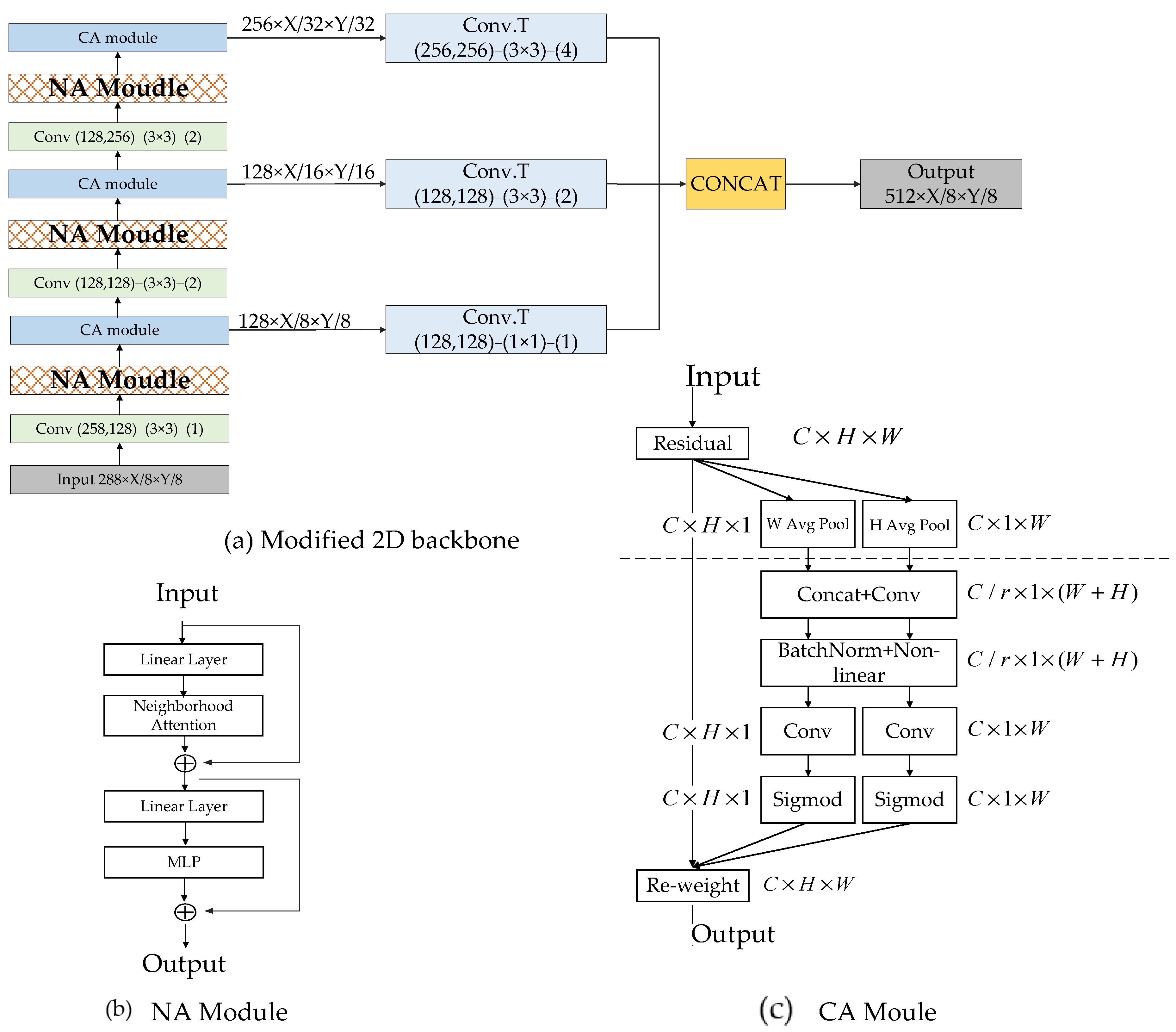
The 2D Backbone: The BEV feature map, which is a 256 × X / 8 × Y / 8 pseudo-image representation that is transformed from the 3D feature map, is the input for the 2D backbone. X and Y mean the original input to the 3D backbone. The 2D backbone consists of two stages for extracting multi-scale features. Specifically, each stage starts with a 3 × 3 downsampled convolution layer for 2× downsampling; the following five 3 × 3 convolutions are used for feature extraction. BatchNorm and ReLU layers are applied after each of the five 3 × 3 convolutional layers. We then upsample the output of each stage to a feature map with the same size and concatenate these feature maps into one feature map. Compared with the original 2D backbone, our improvements are mainly reflected in the 2 OA modules. We use a 64-dimension NA module and a 128-dimension NA module to obtain multi-scale information including cross-channel, direction-aware, and position-sensitive information. The modified 2D backbone is presented in Figure 4.

3.2. Voxel Density-Aware Module

3.2.1. Original Mean VFE

We assumed that the point cloud encompasses 3D spaces with ranges D, H, and W along the Z-, Y-, and X-axes, respectively. We defined each voxel of size v D , v H , and v W accordingly. The resulting 3D voxel grid has the size: D = D / v D , H = H / v H , W = W / v W . Thereafter, the points were grouped according to the voxel they occupy. To balance the number of points within a voxel, if a voxel has more than five points, it needs to be downsampled to five points.
The voxel feature is denoted as V = f i = x i , y i , z i , r i T 4 i = 1 t , that is, as a non-empty voxel containing tT LiDAR points, where f i contains X, Y, and Z coordinates for the i-th point and r i is the received intensity. The mean VFE indicates the average of the coordinates and intensities of each point, and the coordinate average is used as the center of the voxel.

3.2.2. VDA Module

To add density information, we proposed the VDA module. The density of a point in a point cloud can be defined by the number of points within a fixed distance around the point, or it can be defined by the average distance of a fixed number around the point. In this article, we focus on the number of points. Thus, this work defines the point density as the number of points within the fixed radius of the point. If the original point cloud is used as input, when the query radius is set as 1.2 m, the density of dense points can reach 3000, and the density of sparse points is less than 5, which is negative for extracting features. Thus, we use the voxel-filtered point cloud as our input, which ensures that the density of the point cloud is not too high in dense areas. Considering that the number of point clouds in a single voxel contains less information under the current voxel size setting, we adopted a multi-scale method to extract the point cloud density.
As shown in Figure 4a, to reduce the computational cost, we first added the virtual center point (red point) of the voxel in the point cloud set. The number of points in a sphere with a fixed radius r at a certain point is defined as the density of the point.
As illustrated in Figure 4b, to better model the interaction between the point and the surrounding points in different ranges, we used a multi-scale method to extract the density feature of the center point. Multi-scale means that the number of point clouds in different-radius spherical regions is used as a multi-scale feature. Figure 4c shows the process of extracting the density features. We used a light 3D sparse convolution with kernel size = 3, stride = 2, and depth = 16. Then the density features extracted by 3D sparse convolution were projected onto the BEV map through height compression and concatenated with the original BEV features from the sparse convolution network.

3.3. Modified 2D Backbone

3.3.1. Neighborhood Attention (NA)

NA is a simple and flexible attention mechanism for vision; it localizes the receptive field for each token to its neighborhood. We adopt NA based on the reality of 3D object detection: it has no physical correlation with another vehicle for a LiDAR point cloud object. Although in some datasets it may be possible to include certain implicit data through global attention, this will affect the generalization of the model. Therefore, coarse-grained global attention is not necessary for 3D object detection. For a single object, the correlation among the various modules in the object is more significant. Further, owing to the imaging characteristics of LiDAR, object point clouds do not exist on the periphery of the object; thus, none of the objects appear as significantly large or small on the BEV, and their sizes are relatively fixed. Therefore, limiting the receptive field for each token to its neighbor is essential for improving the object detection effect and avoiding high computing costs.
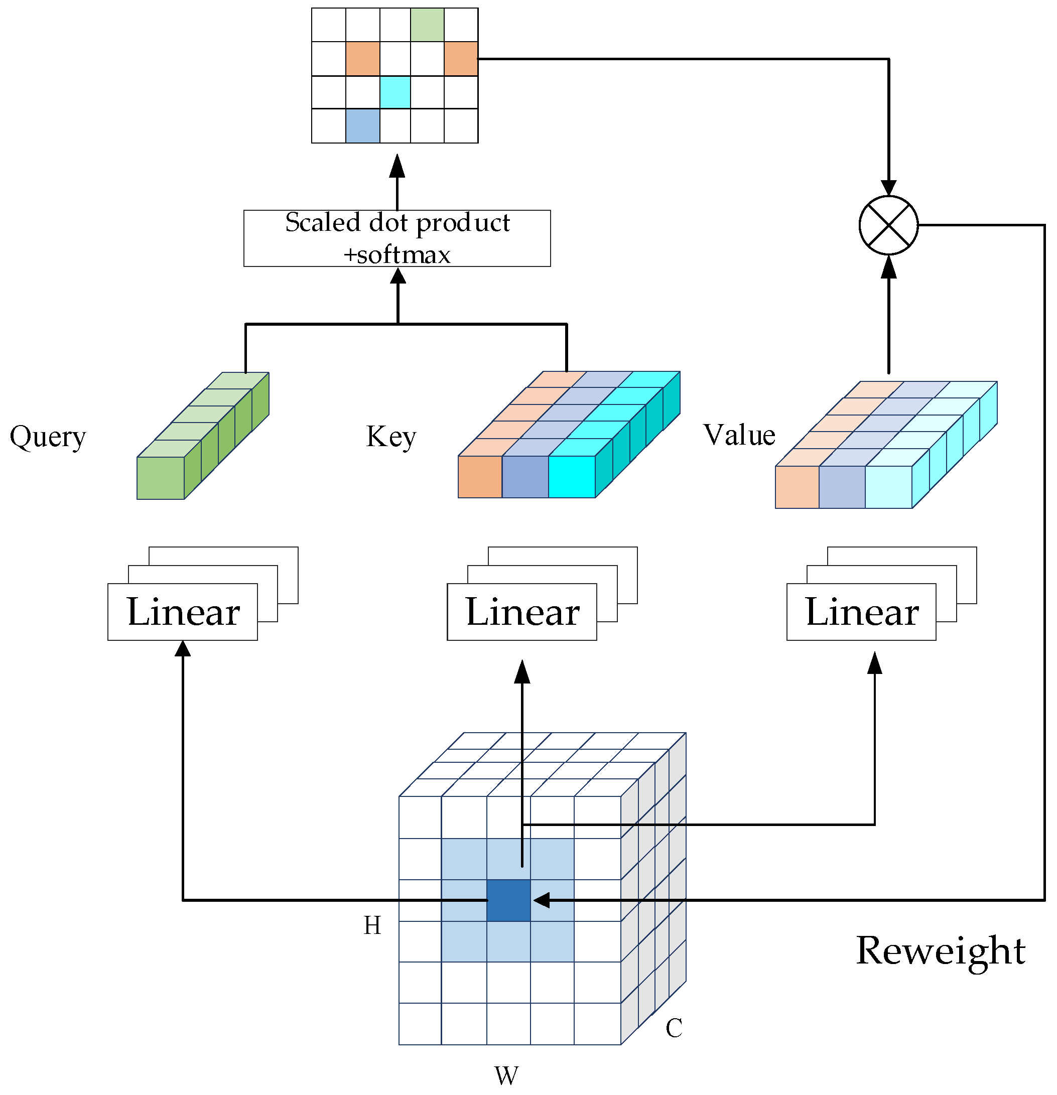
As shown in Figure 5, NA is similar to self-attention. However, each pixel in the BEV map can only attend to its neighboring pixels. H and W represent the length and width of the feature map, respectively, and C represents the number of channels. The neighborhood set of a pixel at (i, j) is denoted as n(i, j), and the length of the neighborhood set is fixed by the kernel size K. For a neighborhood with the size L × L, || n(i, j) || = L2. NA on a single pixel can be defined as follows:
NA X i , j = softmax Q i , j K ρ ( i , j ) T + B i , j s c a l e V n ( i , j )
Here, Q is the linear projection of pixel (i, j), K and V are linear projections of n(i, j), and Bi,j denotes the relative positional bias, which is added to each attention weight based on its relative position. This equation can further be extended to all pixels (i, j), adopting a localized attention form. If the pixel is located at the corner, the neighborhood will also be an L × L grid; however, the query will not be positioned at the center. The computing cost of the original self-attention is O 3 H W C 2 + 2 H 2 W 2 C , whereas that of NA is O 3 H W C 2 + 2 H W C L 2 .

3.3.2. 2D Backbone with Neighborhood Attention and Coordinate Attention

As shown in Figure 6, we modified the 2D backbone by adding NA and CA modules. The NA module can help extract neighboring features, whereas the CA module can aid in embedding the location information into channel attention. The BEV map output from the 3D backbone contains rich spatial information, and the resulting region proposals are important for the final classification and regression analyses. Further, the BEV map is a 3D space extrusion for generating a 2D image; hence, its spatial structure appears with a certain degree of aliasing. Remote spatial interaction information (long-distance interactions) can be captured using accurate location information via coordinate attention; this, in turn, can help in separating the correct target area from the background.

4. Experimental Results

4.1. Dataset and Network Details

ONCE: The ONCE dataset, which was made available in 2021 as an autonomous driving dataset, contains 1 million LiDAR scenes. It uses 40-beam LiDAR and contains rich urban scenes from China. The distribution of traffic participants in this dataset is similar to that in China, and it contains rich weather conditions. Additionally, unlike the simple, medium, and difficult forms of segmentation in the KITTI dataset, the ONCE dataset is divided into three distance ranges: far, medium, and near. In particular, it subdivides vehicles into three classes: cars, buses, and trucks; this detailed division facilitates better testing of the detection performance as it allows for greater inter-class distances and fewer intra-class variations. In our experiments, we considered 4000 sheets for the training set and 4000 sheets for the test set.
KITTI: The KITTI dataset is widely used in the autonomous driving community. It contains 7481 training samples and 7518 testing samples. As the main collection location was a city in Germany, it represents a more ideal environment. According to the division provided by OpenPCDet [18], we divided the 7481 training samples into two further categories, i.e., the training and validation sets, during the process of optimizing the algorithm. The KITTI dataset also contains three categories for detection: cars, pedestrians, and cyclists. It should be noted that as pedestrians and cyclists are fewer in number, their results fluctuate considerably, and the difference between the validation and test sets is large. Hence, we prefer to use the moderately difficult car detection results to measure the performance of the detector. Evaluations of the detection effectiveness for small objects such as pedestrians and bicycles were performed using the ONCE dataset. The authority of the KITTI dataset is ensured by the fact that it strictly limits the number of test results submitted to its official server.
We trained DenNet with a batch size of 8 for 100 epochs, using two Nvidia RTX Quadro 6000 GPUs. The Adam optimizer with a one-cycle policy was used to train our DenNet model. The maximum learning rate was set to 0.003, division factor was set to 10, momentum range was set from 0.95 to 0.85, and weight decay was set to 0.01. The voxel size was set as (0.1 m, 0.1 m, 0.15 m) for the KITTI dataset, whereas it was set as (0.1 m, 0.1 m, 0.2 m) for the ONCE dataset. VDA adopts ball queries with radii of 0.6 m and 1.8 m to extract density features. The kernel size of the NA module was set as 7 × 7.
The average precision (AP) is the main evaluation metric used for object detection models. The evaluations of both the test and validation sets entailed 40 recall positions, represented as AP_40, which is more ideal than the assessment method based on 11 recall positions.

4.2. Results and Analysis

4.2.1. Evaluation with KITTI Dataset

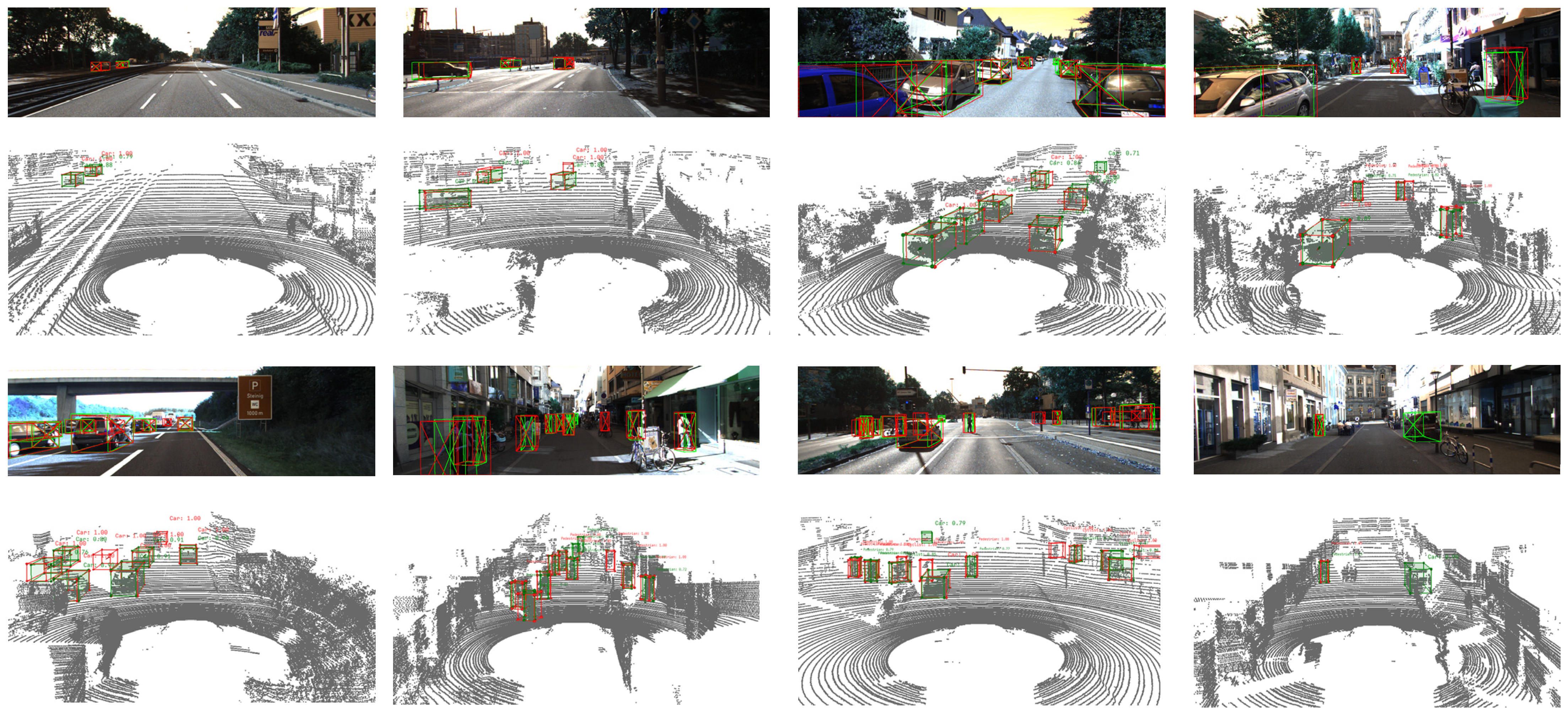
Table 1 shows the results of our DenNet module on the test set of the KITTI dataset. Our method yields competitive results on the KITTI test set when using LiDAR point clouds alone. Specifically, on the KITTI test set, our model achieves AP values of 82.03%, 40.23%, and 64.15% for the vehicle, pedestrian, and cyclist categories at moderate difficulty, respectively. In general, the results obtained are not significantly better than the baseline on the KITTI set. We believe that this might be because the KITTI dataset does not contain sufficient data for training, especially under the vehicle and pedestrian categories. Table 1 shows the results for the validation set of the KITTI dataset. It is important to note the large discrepancy between the validation and test sets for the pedestrian and cyclist detection results. Based on a comparison of the performance of other algorithms under these two categories, we consider the existence of this difference to be acceptable. This was likely caused by the inter-domain differences between the two datasets, given that the number of pedestrians and bicycles is limited in the KITTI dataset. Owing to the limitations in submissions to the official servers of the KITTI dataset, we conducted more extensive experiments on the validation set, as shown in Table 2. As a result, we achieved SOTA results under the cyclist category. Figure 7 shows the qualitative results achieved on the KITTI validation set. It should be noted that after the visualization results, we found that the data annotations of certain pedestrians in the KITTI dataset were not accurate; specifically, some evident pedestrians were not labeled. This may explain the decrease in the accuracy of our model under the pedestrian category.

4.2.2. Evaluation with ONCE Validation Set

Comparison with Baseline: As indicated in Table 3, the mAP of DenNet is 60.31%, which indicates an increase of 3.96% over that of the original Voxel R-CNN. In terms of vehicle detection, the proposed method afforded improvements of 2.81%, 7.97%, and 10.52% for the short, medium, and long distances, respectively, as compared with the baseline. The proposed DenNet also achieved the best detection performance for cyclists, with results 4.20%, 6.01%, and 7.59% higher than those of Voxel R-CNN in the short, medium, and long distances, respectively. By adding the original Voxel R-CNN, in terms of the detection of pedestrians, the average accuracy of DenNet was roughly the same; however, its results were 3.08% and 0.64% better than those of the original Voxel R-CNN in the medium and long distances, respectively. Based on a comparison of the original Voxel R-CNN with the proposed DenNet, it was found that our DenNet performs much better on long-distance and small objects. In particular, for vehicles located at a distance of 50 m, the detection accuracy exceeds the baseline by 10.52%. The visualization results for the ONCE dataset are shown in Figure 8.
Comparison with State-of-the-Art Methods: Table 3 also shows the performance of other SOTA methods on the ONCE benchmark. It can be observed that the proposed method fared well against these SOTA methods in the vehicle categories, which is the most important metric; notably, our proposed method exceeded the second-best results, which come from PV-RCNN, by 0.49%, 1.07%, and 1.85%. Under the cyclist category, the average accuracy of our method was similar to those of the SOTA methods. The performance of our method is better than the central point method in the vehicle and cyclist classes, but not as good as the center-based [27] method in the pedestrian class. This is mainly due to the shortcomings of the anchor-based method. Nevertheless, compared with SOTA methods, it is evident that the proposed DenNet is better at detecting small and far-away instances.

4.3. Ablation Study

Due to the lack of significant changes in the results evaluated on the KITTI dataset and certain errors found in the KITTI labeling, for a detailed comparison of the performance of each proposed module, the ONCE dataset was used for ablation studies. The corresponding results are shown in Table 4. In this case, we adopted the overall mAP of each class of objects as the result.

4.3.1. Effectiveness of VDA Module

After adding the VDA module, the mAP was reduced by 0.46%, as compared with the baseline; in particular, the value for the pedestrian category was 6.72% lower than the baseline. However, the values for the vehicle and cyclist categories showed improvements of 5.29% and 1.39%, respectively. This indicates that the density information, as an important physical quantity, implicitly encodes the distribution of point clouds, thus restoring the loss of point cloud details caused by voxelization, albeit to a certain extent.

4.3.2. Effectiveness of NA and CA Modules

Based on the modified 3D backbone, the proposed NA module and CA module were added to the original 2D backbone. In the first stage, the NA module offers the advantage of self-attention, that is, identifying correlations across different parts. Simultaneously, considering the actual situation of the three-dimensional target, the receptive field is limited to its local area, which significantly reduces the computational time. The mAP of the NA module exceeds that of the original Voxel R-CNN by 2.51%. Multi-scale CA modules model the inter-channel relationships and capture the long-range dependencies with precise positional information; this augments the input features and increases the expressiveness of the object. Thus, the CA modules afforded an improvement of 1.45% over Voxel R-CNN with VDA and NA modules.

5. Conclusions

In this study, a novel, two-stage voxel-based LiDAR 3D object detector, called DenNet, was developed; in particular, DenNet accounts for the importance of densities in 3D detection by introducing the density information of point clouds as an important voxel feature at the initial stages. To better aggregate the information around the voxel, NA in the BEV map was used to explore the relationship between local structures. Furthermore, coordinate attention was also introduced to the inter-channel relationships of the model for capturing long-range dependencies with precise positional information. DenNet afforded better results than SOTA methods on the KITTI and ONCE datasets. The results of this study are expected to serve as guidelines for future 3D object detectors and help understand the significance of density information. Moreover, in industrial applications, our results can help smart cars perceive the surrounding environment better.

Author Contributions

Conceptualization and methodology, H.Q.; validation, H.Q. and X.G.; writing—original draft preparation, H.Q.; writing—review and editing, H.Q., P.W. and S.S.; supervision, X.S.; funding acquisition and resources, X.S. All authors have read and agreed to the published version of the manuscript.

Funding

This work was supported by Hunan Provincial Innovation Foundation for Postgraduate CX20210020 and National Defence University of Science and Technology Intramural Project 2022211.

Conflicts of Interest

The authors declare no conflict of interest.

References

  1. Mao, J.; Shi, S.; Wang, X.; Li, H. 3D Object Detection for Autonomous Driving: A Review and New Outlooks. arXiv 2022, arXiv:2206.09474. [Google Scholar]
  2. Qian, R.; Lai, X.; Li, X. 3D Object Detection for Autonomous Driving: A Survey. Pattern Recognit. 2022, 130, 108796. [Google Scholar] [CrossRef]
  3. Li, J.; Hu, Y. A Density-Aware PointRCNN for 3D Object Detection in Point Clouds. arXiv 2020, arXiv:2009.05307. [Google Scholar]
  4. Ning, J.; Da, F.; Gai, S. Density Aware 3D Object Single Stage Detector. IEEE Sens. J. 2021, 21, 23108–23117. [Google Scholar] [CrossRef]
  5. Hu, J.S.; Kuai, T.; Waslander, S.L. Point Density-Aware Voxels for Lidar 3d Object Detection. arXiv 2022, arXiv:2203.05662v2. [Google Scholar]
  6. Geiger, A.; Lenz, P.; Urtasun, R. Are We Ready for Autonomous Driving? The Kitti Vision Benchmark Suite. In Proceedings of the 2012 IEEE Conference on Computer Vision and Pattern Recognition, Providence, RI, USA, 16–21 June 2012; pp. 3354–3361. [Google Scholar]
  7. Mao, J.; Niu, M.; Jiang, C.; Liang, H.; Chen, J.; Liang, X.; Li, Y.; Ye, C.; Zhang, W.; Li, Z. One Million Scenes for Autonomous Driving: Once Dataset. arXiv 2021, arXiv:2106.11037. [Google Scholar]
  8. Hassani, A.; Walton, S.; Li, J.; Li, S.; Shi, H. Neighborhood Attention Transformer. arXiv 2022, arXiv:2204.07143. [Google Scholar]
  9. Zhou, Y.; Tuzel, O. Voxelnet: End-to-End Learning for Point Cloud Based 3d Object Detection. In Proceedings of the IEEE Conference on Computer Vision and Pattern Recognition, Salt Lake City, UT, USA, 18–23 June 2018; pp. 4490–4499. [Google Scholar]
  10. Yan, Y.; Mao, Y.; Li, B. Second: Sparsely Embedded Convolutional Detection. Sensors 2018, 18, 3337. [Google Scholar] [CrossRef] [PubMed] [Green Version]
  11. Deng, J.; Shi, S.; Li, P.; Zhou, W.; Zhang, Y.; Li, H. Voxel R-Cnn: Towards High Performance Voxel-Based 3d Object Detection. AAAI Conf. Artif. Intell. 2021, 35, 1201–1209. [Google Scholar] [CrossRef]
  12. Shi, S.; Guo, C.; Jiang, L.; Wang, Z.; Shi, J.; Wang, X.; Li, H. Pv-Rcnn: Point-Voxel Feature Set Abstraction for 3d Object Detection. In Proceedings of the IEEE/CVF Conference on Computer Vision and Pattern Recognition, Seattle, WA, USA, 13–19 June 2020; pp. 10529–10538. [Google Scholar]
  13. Mao, J.; Xue, Y.; Niu, M.; Bai, H.; Feng, J.; Liang, X.; Xu, H.; Xu, C. Voxel Transformer for 3D Object Detection. arXiv 2021, arXiv:2109.02497. [Google Scholar]
  14. Mao, J.; Niu, M.; Bai, H.; Liang, X.; Xu, H.; Xu, C. Pyramid R-Cnn: Towards Better Performance and Adaptability for 3d Object Detection. In Proceedings of the IEEE/CVF International Conference on Computer Vision, Montreal, QC, Canada, 6 September 2021; pp. 2723–2732. [Google Scholar]
  15. Gao, F.; Li, C.; Zhang, B. A Dynamic Clustering Algorithm for LiDAR Obstacle Detection of Autonomous Driving System. IEEE Sens. J. 2021, 21, 25922–25930. [Google Scholar] [CrossRef]
  16. Sheng, H.; Cai, S.; Liu, Y.; Deng, B.; Huang, J.; Hua, X.-S.; Zhao, M.-J. Improving 3d Object Detection with Channel-Wise Transformer. In Proceedings of the IEEE/CVF International Conference on Computer Vision, Montreal, QC, Canada, 10–17 October 2021; pp. 2743–2752. [Google Scholar]
  17. Fan, L.; Pang, Z.; Zhang, T.; Wang, Y.-X.; Zhao, H.; Wang, F.; Wang, N.; Zhang, Z. Embracing Single Stride 3d Object Detector with Sparse Transformer. arXiv 2022, arXiv:2112.06375. [Google Scholar]
  18. Team, O.D. OpenPCDet: An Open-Source Toolbox for 3D Object Detection from Point Clouds. Ph.D. Thesis, The Chinese University of Hong Kong, Hong Kong, China, 2020. [Google Scholar]
  19. Lang, A.H.; Vora, S.; Caesar, H.; Zhou, L.; Yang, J.; Beijbom, O. Pointpillars: Fast Encoders for Object Detection from Point Clouds. In Proceedings of the IEEE/CVF Conference on Computer Vision and Pattern Recognition, Long Beach, CA, USA, 15–20 June 2019; pp. 12697–12705. [Google Scholar]
  20. Shi, S.; Wang, X.; Li, H. Pointrcnn: 3d Object Proposal Generation and Detection from Point Cloud. In Proceedings of the IEEE/CVF Conference on Computer Vision and Pattern Recognition, Long Beach, CA, USA, 16–20 June 2019; pp. 770–779. [Google Scholar]
  21. Shi, W.; Rajkumar, R. Point-Gnn: Graph Neural Network for 3d Object Detection in a Point Cloud. In Proceedings of the IEEE/CVF Conference on Computer Vision and Pattern Recognition, Seattle, WA, USA, 13–19 June 2020; pp. 1711–1719. [Google Scholar]
  22. Shi, S.; Wang, Z.; Shi, J.; Wang, X.; Li, H. From Points to Parts: 3d Object Detection from Point Cloud with Part-Aware and Part-Aggregation Network. IEEE Trans. Pattern Anal. Mach. Intell. 2020, 43, 2647–2664. [Google Scholar] [CrossRef] [PubMed] [Green Version]
  23. Liu, Z.; Zhao, X.; Huang, T.; Hu, R.; Zhou, Y.; Bai, X. Tanet: Robust 3d Object Detection from Point Clouds with Triple Attention. AAAI Conf. Artif. Intell. 2020, 34, 11677–11684. [Google Scholar] [CrossRef]
  24. Yang, Z.; Sun, Y.; Liu, S.; Jia, J. 3dssd: Point-Based 3d Single Stage Object Detector. In Proceedings of the IEEE/CVF Conference on Computer Vision and Pattern Recognition, Seattle, WA, USA, 13–19 June 2020; pp. 11040–11048. [Google Scholar]
  25. Chen, C.; Chen, Z.; Zhang, J.; Tao, D. SASA: Semantics-Augmented Set Abstraction for Point-Based 3D Object Detection. arXiv 2022, arXiv:2201.01976. [Google Scholar] [CrossRef]
  26. Zhang, Y.; Hu, Q.; Xu, G.; Ma, Y.; Wan, J.; Guo, Y. Not All Points Are Equal: Learning Highly Efficient Point-Based Detectors for 3d Lidar Point Clouds. arXiv 2022, arXiv:2203.11139. [Google Scholar]
  27. Yin, T.; Zhou, X.; Krahenbuhl, P. Center-Based 3d Object Detection and Tracking. In Proceedings of the IEEE/CVF Conference on Computer Vision and Pattern Recognition, Nashville, TN, USA, 19–25 June 2021; pp. 11784–11793. [Google Scholar]
Figure 1. Comparison between 2D object detection and 3D object detection.
Photonics 09 00820 g001
Figure 2. Proportions of number distributions of points in one voxel for the (a) KITTI set and (b) ONCE set. The X- and Y-axes represent the number of points in a voxel and the proportion of this type of voxel among all the voxels, respectively.
Photonics 09 00820 g002
Figure 3. Illustration of the entire DenNet framework. This framework is based on the original Voxel R-CNN. First, we design the voxel density-aware (VDA) module, which can extract density features. Second, the 2D backbone is optimized by adding the NA and CA modules; the original structure is subdivided into three stages such that additional contextual information can be extracted.
Photonics 09 00820 g003
Figure 4. Diagram of VDA. (a) Relationship between center point and points in other voxels. (b) Mapping of multi-scale density information on BEV map. (c) The process of extracting density features.
Photonics 09 00820 g004
Figure 5. Neighborhood attention.
Photonics 09 00820 g005
Figure 6. Modified 2D backbone. (a) The 2D backbone, where “Conv” denotes the convolutional layer and “Conv.T” represents the transposed convolutional layer. Format of the layer setting follows “channels kernel size -(strides)”. Detailed structure of (b) NA module and (c) CA module.
Photonics 09 00820 g006
Figure 7. Qualitative results achieved on KITTI validation set. Red boxes represent the ground truth, green boxes denote the prediction results, and the numbers in green represent the confidence of the predictions.
Photonics 09 00820 g007
Figure 8. Qualitative results achieved on ONCE dataset. Boxes denote the prediction results.
Photonics 09 00820 g008
Table 1. Performance comparison on the KITTI test set. All results were evaluated based on the mean average precision with 40 recall positions via the official KITTI evaluation server. The best results are presented in bold, whereas the second-best results are underlined.
MethodTypeCar 3D Detection (IoU = 0.7)Ped. 3D Detection (IoU = 0.7)Cyc. 3D Detection (IoU = 0.7)
EasyMod.Hard.EasyMod.Hard.EasyMod.Hard.
SECOND [10]1-stage84.6575.9668.7145.3135.5233.1475.8360.8253.67
PV-RCNN [12]2-stage90.2581.4376.8252.1743.2940.2978.6063.7157.65
PointPillars [19]1-stage82.5874.3168.9951.4541.9238.8977.1058.6551.92
PointRCNN [20]2-stage86.9675.6470.7047.9839.3736.0174.9658.8252.53
PointGNN [21]1-stage88.3379.4772.2951.9243.7740.1478.6063.4857.08
Part-A2 [22]2-stage87.8178.4973.5153.1043.3540.0679.1763.5256.93
TANet [23]2-stage84.3975.9468.8253.7244.3440.4975.7059.4452.53
3DSSD [24]1-stage88.3679.5774.55------
SASA [25]1-stage88.7682.1677.16------
Voxel R-CNN [11]2-stage90.9081.6277.06------
PDV [5]2-stage90.4381.8677.36---83.0467.8160.46
DenNet (Ours)2-stage90.7281.9377.4846.1040.2333.4778.8964.1556.81
Table 2. Performance comparison on KITTI validation set. The best results are presented in bold, whereas the second-best results are underlined.
MethodCar 3D DetectionPed. 3D DetectionCyc. 3D Detection
EasyMod.HardEasyMod.HardEasyMod.Hard
PV-RCNN [12]90.2581.4376.8252.1743.2940.2978.6063.7157.65
3DSSD [24]91.0482.3279.8159.1455.1950.8688.0569.8465.41
IA-SSD [26]91.8883.4180.4461.2256.7751.1588.4270.1465.99
CT3D [16]92.3484.9782.9161.0556.6751.1089.0171.8867.91
PDV [5]92.5685.2983.0566.9060.8055.8592.7274.2369.60
SASA [25]91.8284.4882.0062.3258.0253.3089.1172.6168.19
Voxel R-CNN [11]92.8685.1382.8469.3761.5656.3991.6374.5270.25
DenNet (ours)92.6285.3982.8366.2659.5254.1593.2275.2770.59
Table 3. Performance comparison on ONCE validation set. The best results are presented in bold, whereas the second-best results are underlined.
MethodVehiclePedestrianCyclistmAP
Overall0–30 m30–50 m>50 mOverall0–30 m30–50 m>50 mOverall0–30 m30–50 m>50 m
PointPillars [19]68.5780.8662.0747.0417.6319.7415.1510.2346.8158.3340.3225.8644.34
SECOND [10]71.1984.0463.0247.2526.4429.3324.0518.0558.0469.9652.4334.6151.89
CenterPoints [27]66.7980.1059.5543.3949.9056.2442.6126.2763.4574.2857.9441.4860.05
PV-RCNN [12]77.7789.3972.5558.6423.5025.6122.8417.2759.3771.6652.5836.1753.55
PointRCNN [20]52.0974.4540.8916.814.286.172.400.9129.8446.0320.945.4628.74
IA-SSD [26]70.3083.0162.8447.0139.8247.4532.7518.9962.1773.7856.3139.5357.43
Voxel R-CNN [11]73.5387.0765.5949.9735.6642.3829.8018.1559.8573.5751.5933.6556.35
DenNet (Ours)80.2489.8873.5760.4935.6841.7232.8818.7965.5977.7757.6041.2460.31
Table 4. Ablation study on ONCE validation set.
VDANACAVehiclePedestrianCyclistmAPInference Time (ms)
73.5335.6659.8556.3527.72
78.8228.9461.2455.8932.99
79.9432.2864.3558.8634.68
80.2435.6865.5960.3135.56
Publisher’s Note: MDPI stays neutral with regard to jurisdictional claims in published maps and institutional affiliations.