Abstract
We study the robustness of a nonlinear frequency-division multiplexing (NFDM) system, based on the Zakharov-Shabat spectral problem (ZSSP), that is comprised of two independent quadrature phase-shift keyed (QPSK) channels modulated in the discrete spectrum associated with two distinct eigenvalues. Among the many fiber impairments that may limit this system, we focus on determining the limits due to third-order dispersion, the Raman effect, amplified spontaneous emission (ASE) noise from erbium-doped fiber amplifiers (EDFAs), and fiber losses with lumped gain from EDFAs. We examine the impact of these impairments on a 1600-km system by analyzing the Q-factor calculated from the error vector magnitude (EVM) of the received symbols. We found that the maximum launch power due to these impairments is: 13 dBm due to third-order dispersion, 11 dBm due to the Raman effect, 3 dBm due to fiber losses with lumped gain, and 2 dBm due to these three impairments combined with ASE noise. The maximum launch power due to all these impairments combined is comparable to that of a conventional wavelength-division multiplexing (WDM) system, even though WDM systems can operate over a much larger bandwidth and, consequently, have a much higher data throughput when compared with NFDM systems. We find that fiber losses in practical fiber transmission systems with lumped gain from EDFAs is the most stringent limiting factor in the performance of this NFDM system.
1. Introduction
The spectral efficiency of traditional optical fiber communications systems is limited by the maximum launch power imposed by the Kerr nonlinearity [1]. It is important to investigate techniques that can increase the maximum power, which indicates potential for higher spectral efficiency. An alternative to the use of modulation techniques in optical fiber transmission systems designed for linear systems is the application of nonlinear Fourier transform (NFT) and its inverse (INFT) for the encoding and decoding of digital data in an optical carrier. The NFT is a numerical method that carries out a numerical decomposition of the eigenvalues and the eigenfunctions of the Zakharov-Shabat spectral problem (ZSSP) [2], which is equivalent to the lossless nonlinear Schrödinger equation (NLSE). The NFT is an approach to solve the NLSE in which the phase of the spectral function associated with each eigenvalue evolves linearly along the optical fiber in the presence of the nonlinear Kerr effect. The NFT transforms a waveform into a discrete and a continuous component of the nonlinear spectrum, which comprise the scattering data. The use of scattering data has been proposed as an approach to deal with the nonlinear propagation in optical fibers that could potentially lead to modulation formats with higher spectral efficiency (SE) than currently achievable with existing modulation formats [3].
The lossless NLSE belongs to a a class of integrable nonlinear equations that can be decomposed in their corresponding modes or degrees of freedom, which are denoted the nonlinear spectrum. The nonlinear spectrum of the NLSE can be continous and discrete for anomalous dispersion fibers (negative chromatic dispersion: ), but can only be continuous for normal dispersion fibers (positive chromatic dispersion: ). The discrete modes of integrable nonlinear equations correspond in time-domain to soliton waves, which have been observed in a variety of nonlinear media whose wave propagation is described by integrable nonlinear equations [4,5,6,7,8,9,10,11,12].
There are two approaches for the encoding and decoding of data that can be carried out using the NFT. The NFT can be used to encode data directly on the eigenvalues of the ZSSP at the transmitter using an INFT algorithm, which is decoded with an NFT algorithm at the receiver [13,14,15,16,17,18,19,20,21,22,23]. The other approach uses the NFT as a one-step digital-back-propagation algorithm at the receiver to compensate for the nonlinearity and the dispersion along the fiber [3,24,25,26].
We previously studied the use of one-step digital back-propagation based on the NFT to mitigate the nonlinear Kerr effect in optical fiber communications systems operating in the normal dispersion regime using NFT for data decoding at the receiver while using standard QPSK encoding at the transmitter [26,27] that was based on an earlier work by Turitsyna et al. [24]. We found that the computational cost of this approach becomes unacceptably large at data frame sizes and power levels that are too small to make this approach competitive with current linear transmission schemes [27]. The reason for the rapid increase of the computational cost to encode and decode data in the continuous spectrum of the ZSSP with the launch power and the data frame width results from the exponential dependence of the required spectral resolution with respect to those parameters [27]. Even though more computationally efficient NFT algorithms have been recently developed [28,29,30], the exponential dependence of the number of discrete values of the continuous spectrum required to represent a waveform using the NFT with respect to the launch power and the data frame width limits the practical application of the NFT even if an NFT algorithm reaches the same computational complexity of the fast Fourier transform.
In [31], Zhang and Kschischang showed simulation results of an NFDM subsystem with continuous spectrum modulation in an optical fiber transmission system with lumped amplification. Optimum performance was obtained using a linear minimum mean-squared error (LMMSE) receiver to minimize the correlation between the sub-carriers. Continuous spectrum modulation of the ZSSP has led to high spectral efficiency, but only over narrow bandwidths (5 GHz) with a low optimum launch power ( dBm) [31]. Moreover, the maximum propagation distance of this NFDM system was only 960 km, which is short compared to the propagation distance of transoceanic WDM systems. Kamalian et al. [32] demonstrated an implementation of the periodic NFT. However, the performance limits of that algorithm need to be investigated to compare its performance against that of conventional NFT algorithms. Those studies considered only a single channel.
In this work, we investigate the effectiveness of discrete spectrum modulation in the presence of several fiber impairments that are not included in the ZSSP. The NFT is used to encode data directly on the eigenvalues of the ZSSP at the transmitter using an INFT algorithm, which is decoded with an NFT algorithm at the receiver. A form of discrete spectrum modulation was investigated in the past, where it was referred to as eigenvalue communication [33]. More recently, several groups have studied variations of this approach [13,16,31,34,35,36]. It is important to note that there are other modulation techniques that use the continuous spectrum alone [37] and some recent work have also studied the combination of those two techniques, potentially increasing spectral efficiency as in [38,39]. In [39], experiments with dual polarization showed that the use of NFT only achieved maxiummu launch power of dBm over 3200 km for a system with a total transmission rate of GBb/s. However, these recent studies indicate that data encoding using the NFT approach is still not competitive for systems operating in the anomalous dispersion regime when compared with conventional encoding method similarly to what we have showed in [27] for a system operating in the normal dispersion regime.
The method used by Dong et al. [35], Hari et al. [16] and Leible et al. [23] is an on-off-keyed (OOK) modulation format of multiple eigenvalues. Their methods utilize symbols defined by different combinations of eigenvalues, generating a variety of solitons of different orders. In [16], the authors investigated the characteristics of symbols formed with a combination of up to 5 eigenvalues out of 50, choosing only the pulses/symbols that met specific pulse duration and bandwidth requirements in a single polarization. This method achieved a spectral efficiency of bits/s/Hz. Even though this method does not encode information on the phase of the discrete spectrum, it does initially set the adjacent solitons so that they are as out of phase as possible at the transmitter. However, the spectral efficiency was only calculated at the transmitter and did not take into consideration any change of the pulse duration or bandwidth that occurs during propagation. This neglect of the propagation effects is only possible when the dispersion length () is much larger than the system length, which significantly limits the maximum launch power used in this system.
Shevchenko et al. [40], Gui et al. [41], and Buchberger et al. [42] investigated the performance of high-order modulation in a single soliton, while Bülow et al. [34], Span et al. [43], Gui et al. [20], and Geisler et al. [44] investigated high-order modulation in multiple eigenvalues of the ZSSP. In the approach described by Bülow et al. [34], the phases of the spectral function of two eigenvalues of the discrete spectrum of the ZSSP are modulated. In that study, two independent quadrature phase-shift keying (QPSK) signals are modulated onto each of the two eigenvalues of second-order solitons. That method utilizes more degrees of freedom but still has a low spectral efficiency: bits/s/Hz at the receiver.
Gui et al. showed that modulation in leads to an increase in the maximum propagation distance by about 24% when compared with modulation in the spectral function at BER equal to in a 2-Gbaud 16-QAM transmission on the eigenvalue [20]. However, when the linear minimum mean square error (LMMSE) estimator of the noise in is used, the maximum propagation distance of the system is further improved by 32%, which leads to a maximum propagation distance of 1400 km.
Bülow et al. showed that independent modulation in leads to a better performance than modulation in in a system that consists of 64-QPSK modulated 2-eigenvalue in an ideal lossless optical fiber system with distributed noise [22]. Since the performance of that system was limited by the nonlinear coupling of the signal encoded in the two eigenvalues due to noise, they also observed a significant improvement in the performance of that systems when the signals encoded in the two eigenvalues were jointly detected. When joint detection was used, the system with the signal encoded in of the two eigenvalues led to a maximum propagation distance of , where is the breath length of the eigenvalues at the achievable information rate (AIR) of 11 bit/symbol. That propagation distance is 17% better than that obtained with joint detection of signals encoded in . Those studies also considered only a single channel modulating an optical carrier.
In [45], Yousefi and Yangzhang showed that optical fiber communication systems with NFDM have higher achievable information rates when compared with Wavelength-division multiplexing (WDM). However, that study did not include several of the optical fiber impairments that are not included in the ZSSP. In this paper, we investigate the effectiveness of using the discrete spectrum of the ZSSP to encode data in optical fiber communications systems with two eigenvalues, as was proposed in [34], at length scales that are longer than the dispersion length scale. We utilize a nonlinear frequency division multiplexing (NFDM) system that was introduced by Yousefi et al. [3,46,47] and a transmitter/receiver model that was introduced by Bülow et al. [34]. The transmitter/receiver signal is a second-order soliton with two QPSK signals per symbol that are modulated independently onto each of the two eigenvalues. We use this model system to assess the maximum power level that can be achieved with the system in [34] in the presence of fiber impairments—the Raman effect [48], third-order dispersion, and fiber losses with lumped gain and ASE noise from EDFAs. One significant limitation of eigenvalue encoding is the decrease in the optical intensity along a span length due to the fiber loss in optical transmission systems with lumped amplification. This decrease in the optical intensity along a span length effectively changes the local eigenvalues along the direction of propagation. In [49], Bajaj et al. proposed the use of dispersion decreasing fibers, in which the effective area of the fiber is decreased along the propagation distance. This approach enabled the mitigation of the variation of the nonlinear spectrum along a span length, since the magnitude of the chromatic dispersion decreases while the nonlinear parameter increases along the propagation direction. However, this system with the proposed dispersion decreasing fibers only improves the system performance by 2 dB over a propagation distance of 1280 km when compared to the optimized path-averaged nonlinear parameter approximation that can be used with conventional fibers [49]. We have not considered the impact of dual-polarization multiplexing nor polarization-mode dispersion effects in this system, which have been studied in [36,39,50,51,52,53,54]. The 2-eigenvalue QPSK modulation format has a relatively small SE, which is about bits/s/Hz, but it can in principle be increased by adding more eigenvalues (higher-order soliton) and/or by using a more complex quadrature amplitude modulation (QAM) applied to the spectral function of each eigenvalue. However, the increase in the number of eigenvalues may affect the robustness of this method in the presence of fiber impairments, since the peak-to-average power ratio (PAPR) of the waveform is expected to increase with the number of eigenvalues. We also investigated that effect by adding a third eigenvalue to the NFDM system whose phase is also encoded with another independent QPSK signals.
2. Theory and Numerical Methods
2.1. Channel Model
The slowly-varying envelope of the optical field in an optical fiber, , is described by the generalized NLSE [38,55]:
where , , , and , are the chromatic dispersion, third-order dispersion, the Kerr nonlinearity coefficient, and the Raman parameter, respectively. We set dB/km, ps/km, ps/km, fs, and (W.km), which are standard parameters for dispersion-shifted fibers (DSF). In the case of a single soliton, the relevant soliton parameters are:
where is the time-scale parameter, is the dispersion parameter, and is the peak power of the soliton. Equation (2) defines the relationship between the soliton peak power and the time window/duration of a soliton pulse, as shown in [13,56].
The normalization parameters used for the Darboux transformation, which are applicable to multiple eigenvalues of the ZSSP, are defined by the following normalization rules:
where , and are the normalized amplitude, the normalized propagation distance, and the normalized time, respectively. The value of is a free parameter used for adjusting the transmission rate and consequently the launch power . The relationship between and is defined by:
In general, the NFT of the signal yields both the discrete and continuous spectral components. The discrete spectrum corresponds to the solitonic (non-dispersive) component of the signal. Hence, a waveform that is generated from the discrete spectrum of the ZSSP consists of one or more solitons. The discrete spectrum consists of a finite number of eigenvalues and an equal number of spectral function values , where and are both complex [46].
2.2. Signal Generation
We consider a system with fixed eigenvalues on the imaginary axis (zero real part) and we modulated the values of the spectral function with QPSK constellations. As in [34], we used two eigenvalues, and , to generate a second-order soliton waveform with an independent QPSK modulation of the value of each respective spectral function . Figure 1 shows an example of a second-order soliton waveform.
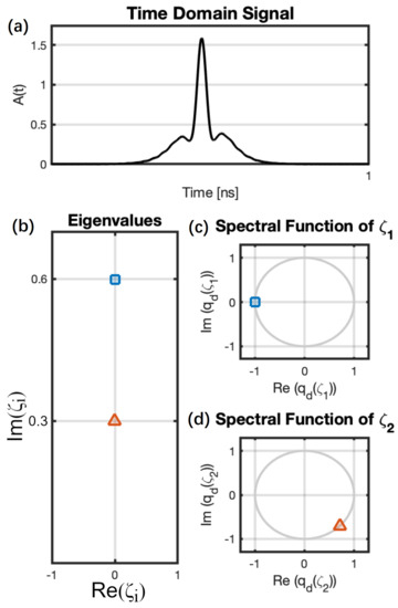
Figure 1.
Single symbol representation: (a) Time domain representation of the second-order soliton. (b) Eigenvalues represented in the complex plane. Blue square used for and red triangle for . (c,d) the spectral function of the respective , in which the QPSK data is encoded.
The algorithms for the NFT and the inverse NFT (INFT) are based on the Ablowitz-Ladik method and the Darboux transform, respectively [57]. We use the Ablowitz-Ladik method combined with the Newton-Raphson method to recover the eigenvalues and their respective encoded spectral functions at the receiver. The waveform is generated at the transmitter from the eigenvalues and the spectral functions using the Darboux transform.
We used the Darboux transform [13] to generate the waveform of the specific second-order soliton with the information encoded into the phase of the spectral function associated with each of the two discrete eigenvalues with independent QPSK signals, shifted by . The waveform in [34] is generated using 64 GSa/s and pulse width of 1 ns, which corresponds to 64 samples per symbol with dBm of launch power (average power) and an optical filter bandwidth of 33 GHz. This high number of samples per symbol is needed to accurately generate the waveform associated with the eigenvalues. The symbol period, the sampling frequency, and the in-line filter bandwidth are rescaled when we change the normalization parameter . Consequently, is also changed, which defines the different launch power levels. Figure 2 shows a comparison of three different launch power signals in the time domain.
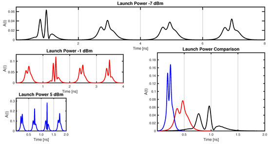
Figure 2.
The black curve on the first plot shows a sequence of 4 symbols in the time domain with launch power of dBm. The red curve in the second plot shows the same sequence but with a launch power of dBm. The blue curve in the third plot shows the same sequence but with a launch power of 5 dBm. The fourth plot on the bottom left shows the first symbol of each of those schemes plotted together for comparison. A launch power increase by a factor of 4 (6 dB) corresponds to a symbol period decrease by a factor of 2, as defined by the relationship of the normalization factors and in (4).
2.3. Performance Measurement
At the receiver, the waveform is up-sampled by interpolation to 1024 samples for the systems with the symbol period and 2048 samples for the systems with symbol period (), in order to meet the NFT resolution requirements at the receiver. Then, we use the Ablowitz-Ladik method at the receiver to calculate the discrete spectrum of the signal and to extract the encoded spectral functions associated with the two received eigenvalues, which include the propagation effects during the transmission. Systems with these specifications are currently too computationally intensive to be practical, but we considered them in this study to determine the performance limits of eigenvalue modulation, given its potential as a tool for nonlinear mitigation. To extract the eigenvalues that were transmitted without having to scan over a large area, the Ablowitz-Ladik method was combined with the Newton-Ralphson method. The combination of these two methods reduces the computational cost in finding the received eigenvalues, which may undergo changes due to fiber impairments that are not included in the ZSSP. The same approach was used in [13,16,34,35,58,59,60].
We use the error vector magnitude (EVM) of the received spectral function of each eigenvalue as the performance measure for the optical fiber impairments considered. The EVM is the root mean square of the deviation of the complex value of a received symbol from its expected value on the complex plane [61]. The EVM is a good indicator of the quality of the received signal in QAM systems. The more spread-out the QPSK constellations are due to the fiber impairments, the larger the EVM is and, consequently, the lower the tolerance of that system to ASE noise is. Note that amplitude deviations that do not affect the phase in QPSK systems increase the EVM without necessarily increasing the bit error rate.
3. Results
For each of the fiber impairments that we considered, we simulated propagation through a 1600 km-long optical fiber transmission system with dispersion equal to ps/km, and with launch powers from dBm to 15 dBm. The schematic representation of the systme that we model is shown in Figure 3. The transmitter and receiver used are adjusted for each launch power, for the same eigenvalues of the ZSSP, because the pulse duration and the receiver bandwidth are different for each launch power as shown in (3). All simulations were performed using a random sequence with 256 symbols. Since each symbol carries 4 bits, each random sequence contains 1024 bits. This sequence was extracted from a pseudorandom binary signal (PRBS11) with length . The same bit string was used for the simulations with different fiber parameters to facilitate the comparison.
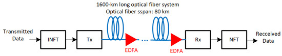
Figure 3.
The schematic representation of an NFDM optical fiber transmission system.
3.1. Baseline Simulation
We first carried out a baseline simulation without including any of the physical impairments of a practical optical fiber transmission system, which corresponds to (1) with , , and R all set equal to zero. The modulation format contains two independent signals, each associated with a different eigenvalue, and we obtain the reciprocal of the EVM for both signals. Figure 4 shows the performance of the baseline simulation as a function of the propagation distance and the launch power. Figure 4a shows the reciprocal of the EVM of the first eigenvalue, , and Figure 4b shows the reciprocal of the EVM of the second eigenvalue, .
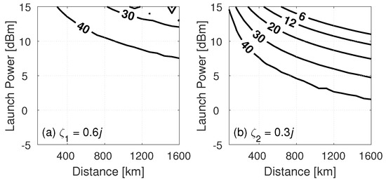
Figure 4.
Performance of the baseline systems as a function of the distance. We show (a) The reciprocal of the EVM in dB for the eigenvalue and (b) The reciprocal of the EVM in dB for the eigenvalue . The level curves in these two sub-figures are for the following values of the reciprocal of the EVM: 6, 12, 20, 30 and 40 dB.
In principle, the reciprocal of the EVM associated with the eigenvalues of the ZSSP should not decay as the signal propagates along an ideal lossless fiber. However even the baseline simulation exhibits some distortion at the receiver at long distances. In Figure 4a,b we observed a reduction of the reciprocal of the EVM as the launch power and the propagation distance increase, which primarily affects the eigenvalue , because it is the eigenvalue associated with the broader component of the second-order soliton waveform. This degradation is due to the finite size of the time window used to represent the waveform, which leads to both truncation errors and inter-symbol interference (ISI). The ISI is due to the finite separation between neighbor symbols, which affects the breathing of the second-order solitons. This ISI includes the interaction among neighboring second-order solitons that is described in [62]. As the launch power increases, the second-order soliton breathing period decreases. Therefore, there are more second-order soliton periods in the same propagation distance and the waveform degrades.
3.1.1. Mitigating Inter-Symbol Interference and Truncation Errors
To investigate the combined effects of ISI and truncation errors, we studied the performance of the same system with twice the symbol period. We denote the symbol period as the symbol period of the system that corresponds to that in [34], while the system with symbol period corresponds to the same waveform with twice the symbol period but with the same sample rate. In Figure 5, we compare the systems with these two symbol durations and with the different number of points that we used to discretize the FFTs and the NFT methods that we used in the simulations.

Figure 5.
The reciprocal of the EVM of the baseline system as a function of the launch power when the system does not include any effects beyond those included in the ZSSP. (a) Results of signal decoded from the first eigenvalue . (b) Results of signal decoded from the second eigenvalue . Results are shown for the system with symbol period equal to and for the system with symbol period equal to .
With symbol period , the reciprocal of the EVM of the second eigenvalue shown in Figure 5b drops below 6 dB at 11 dBm of launch power at 1600 km of propagation distance, while the system with twice the symbol period, , still has the reciprocal of the EVM close to 45 dB at 14 dBm of launch power, in which the EVM is negligible. Since our goal is to investigate the impact of each of the fiber impairments, we study systems with symbol periods and , which allows us to separate the effects that are due to ISI from the other effects. The results in Figure 5 show that convergence was achieved for the case with using points to discretize the waveform even with 12 dBm of launch power. These results also show that convergence was achieved for the case with using points to discretize the waveform even with 12 dBm of launch power. To ensure accuracy in all the simulation results, we discretized all the waveforms used in this study with points.
The value of the reciprocal of the EVM in Figure 5a,b increases when the symbol period doubles with the same sample rate, at the expense of decreasing the SE by half. This performance improvement results from a more accurate representation of the second-order soliton as the symbol period increases, which reduces the ISI due to the tails of adjacent symbols. Since there was no noticeable improvement in the performance when the number of points used to discretize the FFT and the NFT was increased, the number of points was not a limiting factor in the performance of the system. There is a background error in the received signal in Figure 5 that causes the reciprocal of the EVM to oscillate between 45 dB and 60 dB when the symbol period is equal to due to discretization errors in the algorithms. However, the EVM is negligible in that case.
3.1.2. Constellation Analysis
Figure 6a–d show the impact of ISI on the waveform and on the decoded QPSK signal. The waveform is transmitted over 1600 km of propagation distance with 11 dBm of launch power. The results shown in Figure 6a–c use , and the results shown in Figure 6d–f use .
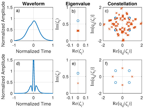
Figure 6.
Simulation of the baseline system at 1600 km of propagation distance with launch power 11 dBm. (a–c) Results with . (d–f) Results with for the same launched symbol. (a,d) Received waveform of one symbol of the sequence. (b,e) Received eigenvalues. (c,f) Normalized received spectral function evaluated at the two eigenvalues: in blue circles and in red crosses.
Figure 6b shows eigenvalues did not change significantly after 1600 km of fiber propagation with 11 dBm of launch power. So that the eigenvalues were properly recovered at the receiver and are not affected by inter-symbol interference with the shorter symbol period . The eigenvalue is shifted more than the eigenvalue because the portion of the waveform more closely related to the eigenvalue is significantly broader than the portion of the waveform associated to . For this reason, the eigenvalue is more susceptible to suffer from ISI than the eigenvalue when the symbol period is reduced. The higher susceptibility to errors of the eigenvalue is shown in Figure 6c, in which the constellations of (blue) are significantly less dispersed than the constellations of (red). The same symbols were launched in the simulations with and in the simulations with in Figure 6a,b. Since the waveforms with and with in this comparison have the same launched power, they have different peak powers and, consequently, different breathing periods. Therefore, after propagating 1600 km along the fiber, the received waveforms are likely to be different.
3.2. Raman Effect
Figure 7 shows how the Raman effect limits the launch power of a system with 1600 km of propagation distance [48]. In this study, we do not include any other effect that is not included in the ZSSP. ISI limits the performance of this system with symbol period for launch power levels above 11 dBm at the 1600 km of propagation distance even when no other fiber impairment is included. Hence, we carried out simulations with symbol periods equal to and in order to isolate its impact.
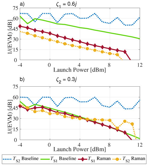
Figure 7.
The reciprocal of the EVM as a function of the launch power when the system only includes the Raman effect. (a) Results of a signal that is decoded from the first eigenvalue . (b) Results of a signal that is decoded from the second eigenvalue . We show results for the system with symbol period equal to and for the system with symbol period equal to .
We compare the case with symbol period , which corresponds to that in [34], and the case with the doubled symbol period with their corresponding baseline cases. The Raman effect has a stronger impact in the performance of the eigenvalue in the case with symbol period , since this eigenvalue is associated with a higher peak power than . However, when the symbol period is , the Raman effect significantly impacts both eigenvalues, since they have higher peak power for the same launch power when compared with the case with symbol period . In a system with either of these two symbol periods, the Raman effect limits the performance of the system to launch powers below 11 dBm.
The system with the smaller symbol period outperforms the system with the larger symbol period as shown in Figure 7a. This performance difference occurs because the simulation with symbol period has significantly higher peak power than that of the simulation with to correspond to the same launch power. The Raman effect causes a shift in the spectrum of the waveform towards longer wavelengths. The narrow portion of the waveform with higher instantaneous power, which is associated with the larger eigenvalue, moves more slowly due to changes in its group velocity due to the Raman effect [63].
Constellation Analysis
Since this coding scheme generates a second-order soliton, the portion of the waveform associated with each individual eigenvalue may propagate with a different group velocity when subjected to fiber impairments such as the Raman effect. The Raman effects disturbs the equilibrium of the interaction forces of the individual solitons in the second-order soliton. As a consequence, the second-order soliton breaks apart into two individual solitons [64,65].
When the propagation distance is long enough or the launch power is high enough, the main lobe of one of the two components of the second-order soliton reaches the neighboring symbol due to the Raman effect. Once that happens, the ISI due to the Raman effect leads to errors in the symbol decoding. Before the total collapse of this modulation scheme due to ISI, the pulse shift inside the symbol time window due to the Raman effect changes the amplitude of the spectral function of at least one of the eigenvalues. This change in the amplitude of increases linearly with the propagation distance until the onset of ISI precludes the use of QAM with multiple levels of amplitude modulation and, consequently, limits any further increase in the SE.
The larger shift in the amplitude of the spectral functions for the case in which the symbol period is equal to , compared to that in which the symbol period is equal to , occurs because the former system with the larger symbol period has a higher peak power for the same launch power.
The changes in the value of the eigenvalues due to the Raman effect do not make them cross the threshold of inter-eigenvalue interference, where one eigenvalue would be mistakenly taken as the other, at the propagation distance and launch powers that we considered. However, the Raman effect significantly changes the eigenvalue from its original value . Hence, the Raman effect would significantly limit the performance of modulation schemes in which information is encoded in the location of the eigenvalues in the complex plane.
Note, however, that most of the shift in the spectral function of the eigenvalues is deterministic and could be taken into account when designing the symbols to optimize the choice of the magnitude and the phase, as long as this shift is not large enough to lead to decoding errors due to ISI.
The constellations of , shown in blue in Figure 8c, maintains approximately the same phase for , but have different amplitudes due to the Raman effect. The 16 different symbols have four starting patterns determined by the phase difference between the two components of the second-order soliton. This phase difference determines the shape of the waveform at the starting point of the breathing period. In Appendix A, we address how one can recognize these patterns and how one can mitigate for those deterministic shifts in the amplitude of the phase function before the onset of decoding errors due to ISI.
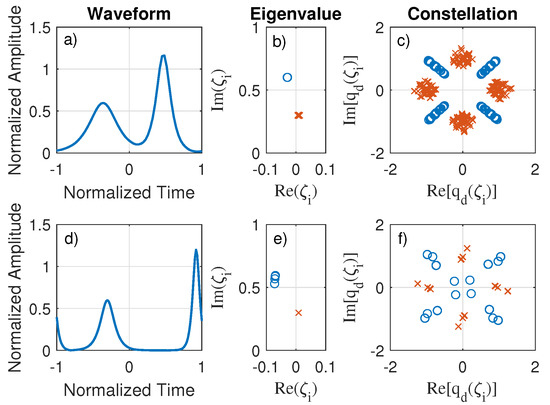
Figure 8.
Simulation with the Raman effect at 1600 km of propagation distance with 9 dBm of launch power. (a–c) Results for the symbol period . (d–f) Results for the symbol period . (a,d) Received waveform for one symbol of the sequence. (b,e) Received eigenvalues. (c,f) Normalized received spectral function constellations, (blue circles) and (red crosses).
In contrast to the constellations of , the constellations of , shown in red in Figure 8c, are spread equally in both amplitude and phase. At this propagation distance and launch power, the ISI that is observed in the baseline simulation is the primary cause of the spread of the constellatons of .
For the system with symbol period , in which the ISI is virtually absent, the constellations of both and are altered by the Raman effect. The constellations of are more strongly affected by the Raman effect than the constellations of , because the former is related to the component of the second-order soliton that has a higher peak power than the latter.
3.3. Third-Order Dispersion
The impact of third-order dispersion in the eigenvalue encoding is also investigated with the two different symbol periods and when it is added to the baseline simulation. Figure 9 shows the impact of third-order dispersion as the power increases. For symbol period , third-order dispersion with 12 dBm of launch power causes a decrease in the reciprocal of the EVM by more than 30 dB when compared to the baseline simulation without any fiber impairments. Third-order dispersion alone can cause the 1600-km-long communication system to fail at launch powers higher than 13 dBm. The performance degradation due to third-order dispersion of the eigenvalue encoding as the launch power increases is due to the increase of the bandwidth with the launch power that is required to generate a second-order soliton waveform.
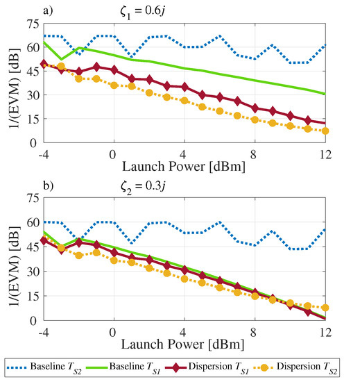
Figure 9.
The reciprocal of the EVM as a function of the launch power when only the third-order dispersion is included. (a) Results of the signal that is decoded from the first eigenvalue . (b) Results of the signal that is decoded from the second eigenvalue . Results are shown for the system with a symbol period equal to and for the system with a symbol period that is equal to .
Constellation Analysis
To study how the third-order dispersion impacts the signal, we obtained the QPSK constellations and the waveforms shown in Figure 10. The eigenvalue locations do not shift at 12 dBm of launch power after 1600 km of propagation distance. However, the spectral function constellations undergo a significant spread, which causes the reciprocal of the EVM to decrease significantly.
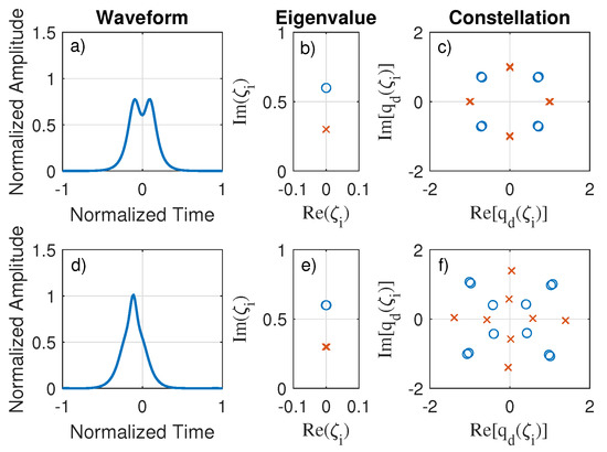
Figure 10.
Simulation results with a symbol period equal to at 1600 km of propagation distance. The system includes only the third-order dispersion. (a–c) Results a with launch power of 1 dBm. (d–f) Results with a launch power of 12 dBm. (a,d) Received waveform of one symbol of the sequence. (b,e) Received eigenvalues. (c,f) Normalized received spectral function constellations, (blue circles) and (red crosses).
The third-order dispersion causes a second-order soliton to shift in the time domain, resulting in a different amplitude at the discrete spectrum constellation. This spread in amplitude affects the possibility of more complex QAM formats, and thus limits the SE. The maximum launch power due to the third-order dispersion is 13 dBm with symbol period .
3.4. Lumped Gain
To address the impact of fiber losses with lumped gain from the EDFAs, it is necessary to adjust the launched waveform because the effective nonlinearity of the fiber is lower than that of a lossless fiber with the same launch power. This decrease in the effective nonlinearity occurs because the average power of the waveform decreases as the waveform propagates through a fiber with losses. One approach to mitigate the effect of losses is to calculate an average/effective value of the nonlinear coefficient of the fiber and generate the waveform based on that new effective nonlinearity coefficient, as shown in Equation (5), where is the fiber nonlinear coefficient, is the new calculated effective nonlinear coefficient and G the total loss over the fiber span [15].
We calculated that a launch power increase of dB is needed for a 80 km fiber span with an attenuation of dB/km when compared to the ideal lossless fiber transmission system. The effective nonlinear coefficient was used in both the INFT encoding at the transmitter and the NFT decoding at the receiver when fiber losses and lumped gain from EDFAs were included in the simulations. Because the effective nonlinear coefficient in the case with lumped amplification is lower than that of a lossless fiber, the same launch power does not correspond to the same symbol rate in both of these cases as shown in Table 1. The effective nonlinear coefficient can be optimized for a particular launch power and waveform duration because the dependence of the breathing period of the solitons on the launch power. Further studies need to be conducted to determine the potential performance enhancement that can result from this optimization. However, we expect that performance optimization to be limited because the eigenvalues and their respective spectral functions vary with the location of the waveform along any given span of a lossy fiber transmission system and that variation increases rapidly with the launch power.

Table 1.
Symbol rate of the sistems considered in this study for selected values of the launch power.
The results shown in Figure 11, with fiber losses and lumped gain from EDFAs, show a significant decrease of the reciprocal of the EVM with an increase of the launch power. This degradation is due to the breakdown of the lossless fiber approximation. This effect is symbol dependent and the error is larger for symbols with largeer PAPR.
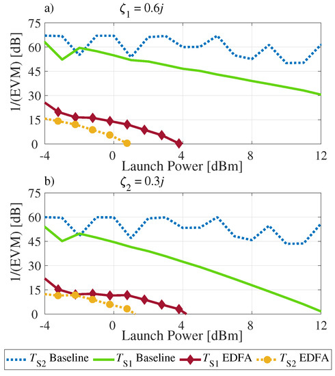
Figure 11.
The reciprocal of the EVM as a function of the launch power when the system includes only fiber losses with lumped gain from EDFAs. (a) Results of the signal decoded from the first eigenvalue . (b) Results of the signal decoded from the second eigenvalue . We show results for the system with a symbol period equal to and for the system with a symbol period equal to .
Constellation Analysis
Because the performance with fiber losses and lumped gain from EDFAs decreases rapidly with the increase of the launch power, we examined the effect of fiber losses and lumped gain in the waveform generated by a symbol that was strongly affected by fiber losses and lumped gain. Figure 12 shows results for dBm of launch power when fiber losses and lumped gain are included. The constellations for both simulations with symbol period and symbol period are almost equally affected because the waveform degradation is not due to ISI. The eigenvalues shown in Figure 12b,e are disturbed even at dBm of launch power, while the constellations are significantly spread out, reducing the reciprocal of the EVM to 10 dB at this low launch power. The signal degradation that affects both eigenvalues is due to the significant deviation of the local eigenvalues of the ZSSP along the fiber due to the decrease in the signal power produced by the losses in the fiber. For that reason, the maximum launch power due to fiber losses with lumped gain is 3 dBm.
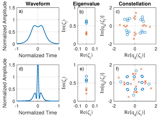
Figure 12.
Simulation results with 1600 km of propagation distance and dBm of launch power. The system includes only fiber losses and lumped gain from EDFAs. (a–c) Results with symbol period equal to . (d–f) Results with symbol period equal to . (a,d) Received waveform of one symbol of the sequence. (b,e) Received eigenvalues. (c,f) Normalized received spectral function constellations, (blue circles) and (red crosses).
Due to errors in the decoding of some of the transmitted symbols using discrete spectrum modulation, Bülow et al. proposed to drop the symbols that are more prone to errors [34]. In that approach to mitigate the errors due to losses and lumped amplification, the symbols with the highest EVM, which correspond to those with high PAPR, are excluded. This procedure decreases the EVM at the expense of the data rate. Another approach to mitigate the impact of fiber losses and lumped gain from EDFAs in the discrete spectrum modulation is to use distributed Raman amplification. Hari et al. have shown that eigenvalues are more robust if distributed Raman amplification is used in a long-haul system, as opposed to EDFA systems [13]. However, distributed Raman amplification schemes have significantly higher cost and much lower energy efficiency when compared to EDFA systems [66,67].
3.5. Ase Noise
In this sub-section, we investigate the impact of ASE noise on the performance of discrete spectrum modulation. This system consists of 20 spans of 80 km with an EDFA at the end of each span. Since the purpose of this study is to characterize the impact of optical noise in the performance of eigenvalue modulation, ASE noise is added at the end of each span, consistent with the amount of ASE noise that is generated in a fiber transmission system with losses and lumped amplification by EDFAs. However, this case is studied without including the losses in the fiber model. To limit the noise bandwidth, the system used an optical filter with a bandwidth of 33 GHz for the case with ns and a launch power of dBm to limit the ASE noise. The symbol period, the sampling frequency, and the in-line filter bandwidth are rescaled with the launch power.
Figure 13 shows the reciprocal of the EVM as a function of the launch power for both eigenvalues and for symbol periods equal to and . The ASE noise limits the maximum power that can be launched in the two-eigenvalue system. The reciprocal of the EVM of the signal encoded in the eigenvalue drops below 6 dB at 1 dBm of launch power, while the reciprocal of the EVM of the signal encoded in the eigenvalue drops below 6 dB at dBm of launch power. The reason why the signal encoded in the eigenvalue is less robust to nonlinear noise [68] when compared with the signal encoded in the eigenvalue is because the former is associated with the second-order soliton component with higher peak power than the latter. The more significant degradation in the performance of the larger eigenvalues due to ASE noise in these results is consistent with the observations in other recent studies [39,51].
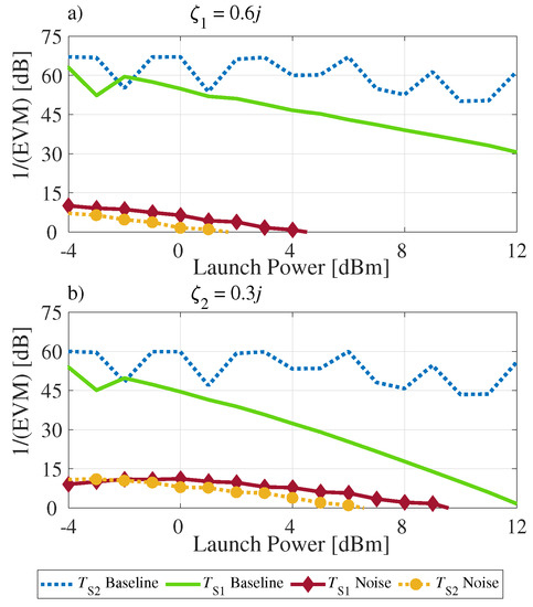
Figure 13.
The reciprocal of the EVM as a function of the launch power when the system includes only ASE noise from EDFAs. (a) Results of the signal decoded from the first eigenvalue . (b) Results of signal decoded from the second eigenvalue .
The impact of optical noise on the discrete spectrum constellation is to spread the amplitude and phase, as well as to displace the location of the eigenvalues. The noise adds more power to the tails of the solitons as well as timing jitter to the pulse peak, leading to a performance degradation, as shown in Figure 13.
3.6. All Impairments Combined
When all the impairments are considered, the performance is limited by the combination of all these effects. However, the losses along the fiber propagation that are compensated by the lumped gain from EDFAs dominates the overall performance degradation, as shown in Figure 14. In essence, the distributed losses have the effect of changing the local eigenvalues of the ZSSP along the propagation distance, which deviates from those of the lossless propagation model of the ZSSP as the launch power increases. The maximum launch power due to all these combined impairments is 2 dBm.
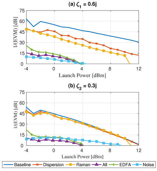
Figure 14.
The reciprocal of the EVM as a function of the launch power when all the effects are included and the symbol period is equal to . (a) Results of the signal that is decoded from the first eigenvalue . (b) Results of the signal that is decoded from the second eigenvalue .
Figure 15 shows the case with . In this case, we have effectively removed the ISI that exists in the baseline system when . The performance with the symbol period is lower by 2 dB when compared to the performance with because the former has twice the symbol period, which means higher peak power, when compared with the latter for the same launch power.
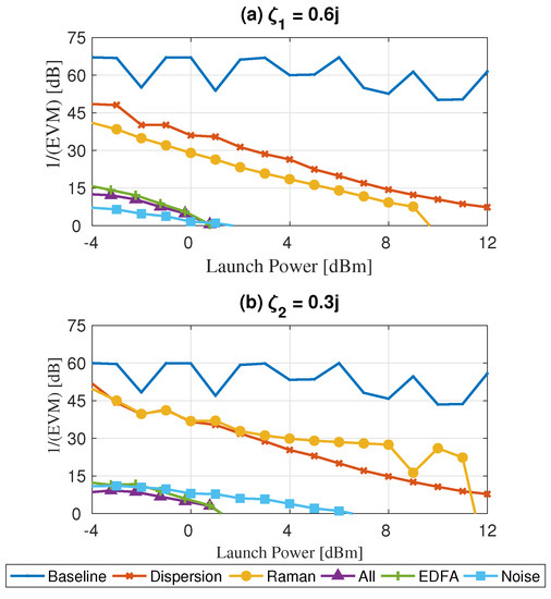
Figure 15.
The reciprocal of the EVM as a function of the launch power when all the effects are included and the symbol period is equal to . (a) Results of the signal decoded from the first eigenvalue . (b) Results of the signal decoded from the second eigenvalue .
We extended this study to include third-order solitons. Due to excessive ISI in this system, it was not possible to use a third-order soliton with symbol period . This means that the increase in the SE enabled by an increase in the number of eigenvalues is partially negated by the need to increase the symbol period for the same launch power. In Figure 16, we shown results for a third-order solition system with symbol period . The maximum launch power due to all the combined impairments in this third-order soliton system is 0 dBm.
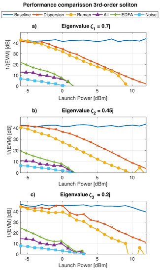
Figure 16.
The reciprocal of the EVM as a function of the launch power when all the effects are included and the symbol period is equal to . (a) Results of the signal that is decoded from the first eigenvalue . (b) Results of the signal that is decoded from the second eigenvalue . (c) Results of the signal that is decoded from the third eigenvalue .
Constellation Analysis
We compare the impact of each effect on the eigenvalue locations and the spectrum constellations at the receiver with the same launch power (around 0 dBm). The constellations reveal that the Raman effect and third-order dispersion have almost no effects at these low launch powers. The fiber losses with lumped gain and the noise are the most significant effects. Figure 17 shows these simulations with symbol period and the constellations for each effect at the receiver with the same launch power level. In Figure 18 we show the constellations of a third-order soliton system with the same launch power, period, and propagation distance shown in Figure 17 for a second-order soliton system.
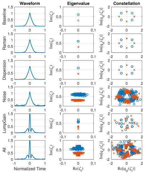
Figure 17.
Simulation results with 1600 km of propagation distance and 0 dBm of launch power for second-order solitons. These results were obtained with a symbol period equal to . The first column shows a waveform of a sampled symbol of the transmitted sequence for each effect respectively. The second column shows the received eigenvalues. The third column shows the normalized received spectral function constellations, (blue circles) and (red crosses).
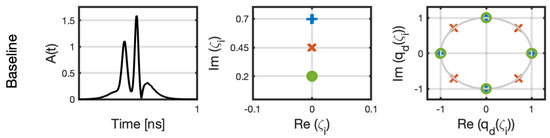
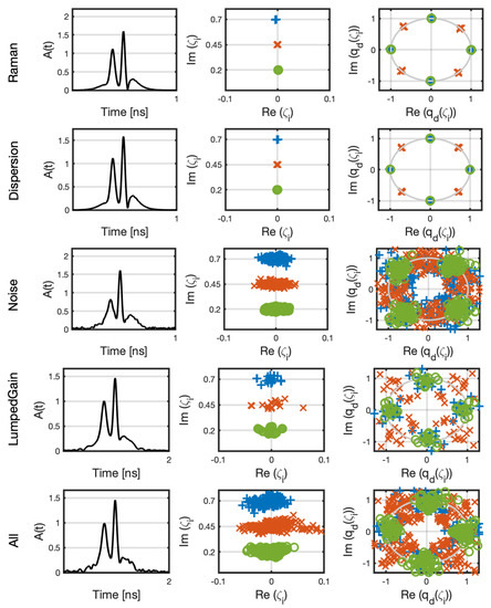
Figure 18.
Simulation results with 1600 km of propagation distance and 0 dBm of launch power for third-order solitons. These results were obtained with a symbol period equal to . The first column shows a waveform of a sampled symbol of the transmitted sequence for each effect, respectively. The second column shows the received eigenvalues. The third column shows the normalized received spectral function constellations, for each of the three eigenvalues.
As observed in the results shown in this sub-section, the QPSK constellations of the systems in which only ASE noise is included are worse than when all the impairments are combined due to the excess nonlinear noise accumulation in the former when compared to the later. In practice, the signal and noise attenuation limit the nonlinear noise accumulation as included in the more realistic case in which all the effects are included. Since the impact of the Raman effect and the chromatic dispersion are not significant at 0 dBm of launch power, those effects did not cause any significant deviation of the QPSK constellations from the baseline results as shown in Figure 17 and Figure 18. Additional studies optimizing the location of the eigenvalues and the symbol period would need to be carried out to determine the absolute performance limit of this NFDM system with discrete eigenvalues with respect to the fiber impairments, but the maximum launch power in the optimized system is expected to decrease with the number of eigenvalues.
4. Conclusions
We show that in an ideal lossless fiber without ASE noise, the Raman effect is the limiting factor of the performance of a modulation scheme based on a two-eigenvalue spectrum modulation, since the Raman effect causes a second-order soliton to break apart, and at least one of the two components of the second-order soliton shifts into a neighboring symbol, leading to ISI. For this modulation format, this ISI occurs when the launch power is higher than 11 dBm when the signal propagates longer than 1600 km. This result suggests that the Raman effect could significantly limit the performance of multi-eigenvalue modulation formats that could be investigated to increase the SE even in systems with distributed gain. We also show that in practical systems with fiber losses and lumped gain and ASE noise from EDFAs, those effects limit the maximum launch power to about 2 dBm. The performance limit of the discrete spectrum modulation format is primarily due to optical fiber losses combined with lumped amplification, which leads to a large deviation of the signal evolution in the optical fiber transmission system from that in the lossless fiber model that is described by the ZSSP. To enhance the SE of eigenvalue spectrum modulation, it would be necessary to increase the number of eigenvalues. However, an increase in the number of eigenvalues requires a longer symbol period due to ISI and, consequently, a higher peak power for the same launch power, which reduces the effectiveness of eigenvalue spectrum modulation. Consequently, the impact of these effects must be considered in any realistic assessment of a system that uses modulation of the discrete spectrum of the ZSSP. We suggest that further studies should be done with alternative decoding methods such as signal processing at the receiver based on neural networks [54,69] and alternative encoding methods to modulate the spectral function of the eigenvalues [20,22], to verify their robustness to the fiber impairments at high launch power levels in long-haul systems, including polarization-mode dispersion effects as well as dual-polarization schemes. All those studies consisted of a single NFDM signal modulating an optical carrier, which corresponds to a single channel. Unlike conventional WDM systems, in which a large number of independently modulated carriers are used, one cannot add independently modulated NFDM signals in different carriers without using some kind of joint detection scheme because those channels would be coupled by the nonlinear Kerr effect [31]. For multi-channel NFDM systems to be competitive with WDM systems, computationally intensive joint detection algorithms would need to be developed. Until an effective multiplexing scheme for NFDM is developed that allows that communication system to be scaled up over a wide bandwidth as in commercially available WDM systems, optimizations of single-channel NFDM systems have limited practical applications.
Author Contributions
Conceptualization, C.R.M., I.T.L.J., V.S.G. and M.O.; methodology, I.T.L.J., T.D.S.D.M. and C.R.M.; software, T.D.S.D.M., C.T. and V.B.; validation, T.D.S.D.M., C.T. and V.B.; writing—original draft preparation, T.D.S.D.M. and I.T.L.J.; writing—review and editing, I.T.L.J. and C.R.M.; supervision, I.T.L.J. and C.R.M.; project administration, I.T.L.J. and C.R.M. All authors have read and agreed to the published version of the manuscript.
Funding
The authors acknowledge partial financial support from Ciena Corporation.
Institutional Review Board Statement
Not applicable.
Informed Consent Statement
Not applicable.
Data Availability Statement
Not applicable.
Conflicts of Interest
The authors declare no conflict of interest.
Appendix A. Pre-Compensation For Raman Shift
The Raman effect breaks apart the second-order soliton and causes the two components of a second-order soliton to drift apart inside the symbol time window. Different symbols with different phases encoded on each eigenvalue will evolve differently, causing the drift to be different for each symbol. This effect is deterministic and can be pre-compensated with a pulse shift at the transmitter. Figure A1 compares the constellation of a regular and a pre-compensated constellation at the receiver when the Raman effect is the only fiber impairment that is considered.
To compensate for the Raman effect, we can adjust the original constellation with a time and phase shift that is sufficient to negate the expected shift in the phase at the receiver. This phase shift depends on the phase difference between the eigenvalues. In Figure A2, we show the results of this technique. This pre-compensation method is effective up to the launch power level in which the time-shift in the eigenvalues due to the Raman effect is not large enough to lead to errors due to ISI.

Figure A1.
Constellations recovered at the receiver after 1600 km of propagation distance with the Raman effect and 10.25 dBm launch power. (a) Results of the received constellations without using any initial compensation. The dots with different colors show all the constellations that arise from the pattern dependence due to the Raman effect. (b) Results of the received constellations with the use of a pre-equalizer technique.


Figure A2.
Waveform of all 16 possible symbols at the receiver when the phase shift is not compensated. There are four different patterns for each initial phase that is encoded in the two eigenvalues. The peak value of the waveforms are shown on the vertical axes in milliwatts, and the corresponding center time of the waveforms relative to the group is shown on the horizontal axes in picoseconds.

References
- Essiambre, R.J.; Kramer, G.; Winzer, P.J.; Foschini, G.J.; Goebel, B. Capacity Limits of Optical Fiber Networks. J. Light. Technol. 2010, 28, 662–701. [Google Scholar] [CrossRef]
- Zakharov, V.E.; Shabat, A.B. Exact theory of two-dimensional self-focusing and one-dimensional self-modulation of waves in nonlinear media. Sov. Phys. JETP 1972, 34, 62–69. [Google Scholar]
- Yousefi, M.I.; Kschischang, F.R. Information transmission using the nonlinear Fourier transform, part III: Spectrum modulation. IEEE Trans. Info. Theory 2014, 60, 4346–4369. [Google Scholar] [CrossRef]
- Redor, I.; Barthélemy, E.; Michallet, H.; Onorato, M.; Mordant, N. Experimental Evidence of a Hydrodynamic Soliton Gas. Phys. Rev. Lett. 2019, 122, 214502. [Google Scholar] [CrossRef] [PubMed]
- Liu, J.; Lucas, E.; Raja, A.S.; He, J.; Riemensberger, J.; Wang, R.N.; Karpov, M.; Guo, H.; Bouchand, R.; Kippenberg, T.J. Photonic microwave generation in the X- and K-band using integrated soliton microcombs. Nat. Photonics 2020, 14, 486–491. [Google Scholar] [CrossRef]
- Wang, W.; Wang, L.; Zhang, W. Advances in soliton microcomb generation. Adv. Photonics 2020, 2, 034001. [Google Scholar] [CrossRef]
- Rozenman, G.G.; Shemer, L.; Arie, A. Observation of accelerating solitary wavepackets. Phys. Rev. E 2020, 101, 050201. [Google Scholar] [CrossRef] [PubMed]
- Rozenman, G.G.; Schleich, W.P.; Shemer, L.; Arie, A. Periodic Wave Trains in Nonlinear Media: Talbot Revivals, Akhmediev Breathers, and Asymmetry Breaking. Phys. Rev. Lett. 2022, 128, 214101. [Google Scholar] [CrossRef] [PubMed]
- Lannig, S.; Schmied, C.M.; Prüfer, M.; Kunkel, P.; Strohmaier, R.; Strobel, H.; Gasenzer, T.; Kevrekidis, P.G.; Oberthaler, M.K. Collisions of Three-Component Vector Solitons in Bose-Einstein Condensates. Phys. Rev. Lett. 2020, 125, 170401. [Google Scholar] [CrossRef] [PubMed]
- Rozenman, G.G.; Fu, S.; Arie, A.; Shemer, L. Quantum mechanical and optical analogies in surface gravity water waves. Fluids 2019, 4, 96. [Google Scholar] [CrossRef]
- Pernet, N.; St-Jean, P.; Solnyshkov, D.D.; Malpuech, G.; Carlon Zambon, N.; Fontaine, Q.; Real, B.; Jamadi, O.; Lemaître, A.; Morassi, M.; et al. Gap solitons in a one-dimensional driven-dissipative topological lattice. Nat. Phys. 2022, 18, 678–684. [Google Scholar] [CrossRef]
- Qi, Y.; Yang, S.; Wang, J.; Li, L.; Bai, Z.; Wang, Y.; Lv, Z. Recent advance of emerging low-dimensional materials for vector soliton generation in fiber lasers. Mater. Today Phys. 2022, 23, 100622. [Google Scholar] [CrossRef]
- Hari, S.; Kschischang, F.; Yousefi, M. Multi-eigenvalue communication via the nonlinear Fourier transform. In Proceedings of the 2014 27th Biennial Symposium on Communications (QBSC), Kingston, ON, Canada, 1–4 June 2014; pp. 92–95. [Google Scholar]
- Le, S.T.; Prilepsky, J.E.; Turitsyn, S.K. Nonlinear inverse synthesis for high spectral efficiency transmission in optical fibers. Opt. Express 2014, 22, 26720–26741. [Google Scholar] [CrossRef]
- Le, S.T.; Prilepsky, J.E.; Turitsyn, S.K. Nonlinear inverse synthesis technique for optical links with lumbed amplification. Opt. Express 2015, 23, 8317–8325. [Google Scholar] [CrossRef] [PubMed]
- Hari, S.; Yousefi, M.I.; Kschischang, F.R. Multieigenvalue Communication. J. Light. Technol. 2016, 34, 3110–3117. [Google Scholar] [CrossRef]
- Bülow, H.; Aref, V.; Idler, W. Transmission of waveforms determined by 7 eigenvalues with PSK-modulated spectral amplitudes. In Proceedings of the European Conference on Optical Communication, ECOC, Dusseldorf, Germany, 18–22 September 2016; pp. 412–414. [Google Scholar]
- Aref, V.; Bülow, H. Design of 2-Soliton spectral phase modulated pulses over lumped amplified link. In Proceedings of the European Conference on Optical Communication (ECOC), Dusseldorf, Germany, 18–22 September 2016; pp. 409–411. [Google Scholar]
- Bülow, H.; Len, S.T.; Aref, V. Modulation of the nonlinear spectrum in experiment. In Proceedings of the Optics InfoBase Conference Papers—Advanced Photonics Conference, New Orleans, LA, USA, 24–27 July 2017; pp. 10–12. [Google Scholar]
- Gui, T.; Chan, T.H.; Lu, C.; Lau, A.P.T.; Wai, P.A. Alternative Decoding Methods for Optical Communications Based on Nonlinear Fourier Transform. J. Light. Technol. 2017, 35, 1542–1550. [Google Scholar] [CrossRef]
- Aref, V.; Le, S.T.; Buelow, H. Modulation over Nonlinear Fourier Spectrum: Continuous and Discrete Spectrum. J. Light. Technol. 2018, 36, 1289–1295. [Google Scholar] [CrossRef]
- Bülow, H.; Aref, V.; Schmalen, L. Modulation on Discrete Nonlinear Spectrum: Perturbation Sensitivity and Achievable Rates. IEEE Photonics Technol. Lett. 2018, 30, 423–426. [Google Scholar] [CrossRef]
- Leible, B.; Chen, Y.; Yousefi, M.I.; Hanik, N. Soliton Transmission with 5 Eigenvalues over 2000km of Raman-Amplified Fiber. In Proceedings of the International Conference on Transparent Optical Networks, Bucharest, Romania, 1–5 July 2018; pp. 1–4. [Google Scholar]
- Turitsyna, E.G.; Turitsyn, S.K. Digital signal processing based on inverse scattering transform. Opt. Lett. 2013, 38, 4186–4188. [Google Scholar] [CrossRef] [PubMed]
- Wahls, S.; Le, S.T.; Prilepsk, J.E.; Poor, V.H.; Turitsyn, S.K. Digital backpropagation in the nonlinear Fourier domain. In Proceedings of the IEEE Workshop on Signal Processing Advances in Wireless Communications (SPAWC), Stockholm, Sweden, 28 June–1 July 2015; pp. 445–449. [Google Scholar] [CrossRef]
- Lima Jr., I.T.; Grigoryan, V.S.; O’Sullivan, M.; Menyuk, C.R. Computational Complexity of Nonlinear Transforms Applied to Optical Communications Systems with Normal Dispersion Fibers. In Proceedings of the 2015 IEEE Photonics Conference (IPC), Reston, VA, USA, 4–8 October 2015; pp. 277–278. [Google Scholar]
- Lima, I.T., Jr.; DeMenezes, T.D.S.; Grigoryan, V.S.; O’Sullivan, M.; Menyuk, C.R. Nonlinear Compensation in Optical Communication Systems with Normal Dispersion Fiber Using Nonlinear Fourier Transform. J. Light. Technol. 2017, 35, 5056–5068. [Google Scholar] [CrossRef]
- Chimmalgi, S.; Prins, P.J.; Wahls, S. Nonlinear Fourier transform algorithm using a higher order exponential integrator. In Proceedings of the OSA Advanced Photonics Congress, Zurich, Switzerland, 2–5 July 2018; pp. 7–8. [Google Scholar]
- Medvedev, S.; Vaseva, I.; Chekhovskoy, I.; Fedoruk, M. Novel numerical algorithm with fourth-order accuracy for the direct Zakharov-Shabat problem. arXiv 2019, arXiv:1902.09736v7. [Google Scholar]
- Wahls, S.; Chimmalgi, S.; Prins, P.J. Wiener-Hopf Method for b-Modulation. In Proceedings of the 2019 Optical Fiber Communications Conference and Exhibition (OFC), San Diego, CA, USA, 3–7 March 2019; pp. 1–2. [Google Scholar]
- Zhang, Q.; Kschischang, F. Correlation-Aided Nonlinear Spectrum Detection. J. Light. Technol. 2021, 39, 4923–4931. [Google Scholar] [CrossRef]
- Kamalian, M.; Vasylchenkova, A.; Prilepsky, J.; Shepelsky, D.; Turitsyn, S. Communication System Based on Periodic Nonlinear Fourier Transform with Exact Inverse Transformation. In Proceedings of the 2018 European Conference on Optical Communication (ECOC), Rome, Italy, 23–27 September 2018. [Google Scholar]
- Hasegawa, A.; Kodama, Y. Solitonsn in Optical Communications; Oxford University Press: Oxford, UK, 1995. [Google Scholar]
- Bülow, H.; Aref, V.; Schuh, K.; Idler, W. Experimental Nonlinear Frequency Domain Equalization of QPSK Modulated 2-Eigenvalue Soliton. In Proceedings of the 2016 Optical Fiber Communications Conference and Exhibition (OFC), Anaheim, CA, USA, 20–24 March 2016; pp. 1–3. [Google Scholar]
- Dong, Z.; Hari, S.; Gui, T.; Zhong, K.Y.M.I.; Lu, C.; Wai, P.K.A.; Kschishang, F.R.; Lau, A.P.T. Nonlinear frequency division multiplexed based on NFT. IEEE Photonics Tehcnol. Lett. 2015, 27, 1621–1623. [Google Scholar] [CrossRef]
- Span, A.; Aref, V.; Bulow, H.; Ten Brink, S. Efficient Precoding Scheme for Dual-Polarization Multi-Soliton Spectral Amplitude Modulation. IEEE Trans. Commun. 2019, 67, 7604–7615. [Google Scholar] [CrossRef]
- Civelli, S.; Forestieri, E.; Secondini, M. A Novel Detection Strategy for Nonlinear Frequency-Division Multiplexing. In Proceedings of the 2018 Optical Fiber Communications Conference and Exposition (OFC), San Diego, CA, USA, 11–15 March 2018; pp. 1–3. [Google Scholar]
- Bülow, H. Experimental demonstration of optical signal detection using nonlinear Fourier transform. J. Light. Technol. 2015, 33, 1433–1439. [Google Scholar] [CrossRef]
- Da Ros, F.; Civelli, S.; Gaiarin, S.; Da Silva, E.P.; De Renzis, N.; Secondini, M.; Zibar, D. Dual-Polarization NFDM Transmission with Continuous and Discrete Spectral Modulation. J. Light. Technol. 2019, 37, 2335–2343. [Google Scholar] [CrossRef]
- Shevchenko, N.A.; Prilepsky, J.E.; Derevyanko, S.A.; Alvarado, A.; Bayvel, P.; Turitsyn, S.K. A lower bound on the per soliton capacity of the nonlinear optical fibre channel. In Proceedings of the ITW 2015—2015 IEEE Information Theory Workshop, Jeju Island, Korea, 11–15 October 2015; pp. 104–108. [Google Scholar]
- Gui, T.; Lo, S.K.; Zhou, X.; Lu, C.; Tao Lau, A.P.; Wai, P.K. High-order modulation on a single discrete eigenvalue for optical communications based on nonlinear Fourier transform. Opt. Express 2017, 25, 20286–20297. [Google Scholar] [CrossRef] [PubMed]
- Buchberger, A.; Graell I Amat, A.; Aref, V.; Schmalen, L. Probabilistic eigenvalue shaping for nonlinear fourier transform transmission. J. Light. Technol. 2018, 36, 4799–4807. [Google Scholar] [CrossRef]
- Span, A.; Aref, V.; Henning, B. On Time-Bandwidth Product of Multi-Soliton Pulses. In Proceedings of the IEEE International Symposium on Information Theory (ISIT), Aachen, Germany, 25–30 June 2017; pp. 61–65. [Google Scholar]
- Geisler, A.; Leibrich, J.; Schäffer, C.G. Influence of non-ideal first order counter-propagating Raman amplification on discrete nonlinear fourier spectrum based communication. In Proceedings of the ITG-Fachbericht—Photonische Netze, Leipzig, Germany, 11–12 June 2018; Volume 279, pp. 83–89. [Google Scholar]
- Yousefi, M.; Yangzhang, X. Linear and Nonlinear Frequency-Division Multiplexing. IEEE Trans. Inf. Theory 2020, 66, 478–495. [Google Scholar] [CrossRef]
- Yousefi, M.I.; Kschischang, F.R. Information transmission using the nonlinear Fourier transform, part I: Mathematical tools. IEEE Trans. Info. Theory 2014, 60, 4312–4328. [Google Scholar] [CrossRef]
- Yousefi, M.I.; Kschischang, F.R. Information transmission using the nonlinear Fourier transform, part II: Numerical methods. IEEE Trans. Info. Theory 2014, 60, 4329–4345. [Google Scholar] [CrossRef]
- DeMenezes, T.D.S.; Grigoryan, V.S.; O’Sullivan, M.; Menyuk, C.R.; Lima Jr., I.T. Performance Limits of a Nonlinear Frequency Division Multiplexed System due to the Raman effect. In Proceedings of the 2017 IEEE Photonics Conference (IPC), Orlando, FL, USA, 1–5 October 2017. [Google Scholar]
- Bajaj, V.; Chimmalgi, S.; Aref, V.; Wahls, S. Exact NFDM Transmission in the Presence of Fiber-Loss. J. Light. Technol. 2020, 38, 3051–3058. [Google Scholar] [CrossRef]
- Gaiarin, S.; Perego, A.M.; da Silva, E.P.; da Ros, F.; Zibar, D. Dual-polarization nonlinear Fourier transform-based optical communication system. Optica 2018, 5, 263–270. [Google Scholar] [CrossRef]
- Gaiarin, S.; Da Ros, F.; De Renzis, N.; da Silva, E.P.; Zibar, D. Dual-Polarization NFDM Transmission Using Distributed Raman Amplification and NFT-Domain Equalization. IEEE Photonics Technol. Lett. 2018, 30, 1983–1986. [Google Scholar] [CrossRef]
- Yangzhang, X.; Lavery, D.; Bayvel, P.; Yousefi, M.I. Impact of Perturbations on Nonlinear Frequency-Division Multiplexing. J. Light. Technol. 2018, 36, 485–494. [Google Scholar] [CrossRef]
- Tavakkolnia, I.; Safari, M. The Impact of PMD on Single-Polarization Nonlinear Frequency Division Multiplexing. J. Light. Technol. 2019, 37, 1264–1272. [Google Scholar] [CrossRef]
- Koch, J.; Chan, K.; Schaeffer, C.G.; Pachnicke, S. Signal Processing Techniques for Optical Transmission Based on Eigenvalue Communication. IEEE J. Sel. Top. Quantum Electron. 2021, 27. [Google Scholar] [CrossRef]
- Agrawal, G.P. Nonlinear Fiber Optics, 3rd ed.; Academic Press: San Diego, CA, USA, 2001. [Google Scholar]
- Keiser, G. Optical Fiber Communications, 4th ed.; McGraw-Hill Education: Berkshire, UK, 2010. [Google Scholar]
- Ablowitz, M.J.; Ladik, J.F. Nonlinear differential-difference equations. J. Math. Phys. 1975, 16, 598–603. [Google Scholar] [CrossRef]
- Bülow, H. Experimental Assessment of Nonlinear Fourier Transform Based Detection under Fiber Nonlinearity. In Proceedings of the 2014 European Conference on Optical Communication (ECOC), Cannes, France, 21–25 September 2014. [Google Scholar]
- Bülow, H. Nonlinear Fourier Transformation Based Coherent Detection Scheme for Discrete Spectrum. In Proceedings of the Optical Fiber Communications Conference and Exhibition, Los Angeles, CA, USA, 22–26 March 2015; pp. 1–3. [Google Scholar]
- Aref, V.; Bülow, H.; Schuh, K.; Idler, W. Experimental Demonstration of Nonlinear Frequency Division Multiplexed Transmission. In Proceedings of the European Conference on Optical Communication, Valencia, Spain, 27 September–1 October 2015; pp. 1–3. [Google Scholar]
- Schmogrow, R.; Nebendahl, B.; Winter, M.; Josten, A.; Hillerkuss, D.; Koenig, S.; Meyer, J.; Dreschmann, M.; Huebner, M.; Koos, C.; et al. Error Vector Magnitude as a Performance Measure for Advanced Modulation Formats. IEEE Photonics Technol. Lett. 2012, 24, 61–63. [Google Scholar] [CrossRef]
- Gordon, J.P. Interaction forces among solitons in optical fibers. Opt. Lett. 1983, 8, 596–598. [Google Scholar] [CrossRef]
- Agrawal, G.P. Applied Nonlinear Fiber Optics; Academic Press: San Diego, CA, USA, 2001. [Google Scholar]
- Gordon, J.P. Theory of the soliton self-frequency shift. Opt. Lett. 1986, 11, 662–664. [Google Scholar] [CrossRef] [PubMed]
- Hause, A.; Mitschke, F. Soliton trains in motion. Phys. Rev. A 2010, 82, 043838. [Google Scholar] [CrossRef]
- Le, S.T.; Prilepsky, J.E.; Rosa, P.; Ania-Castanon, J.D.; Turitsyn, S.K. Nonlinear Inverse Synthesis for Optical Links With Distributed Raman Amplification. J. Light. Technol. 2016, 34, 1778–1786. [Google Scholar] [CrossRef]
- Wang, P.; Hinton, K.; Farrell, P.M.; Pillai, B.S.G. On EDFA and Raman Fiber Amplifier Energy Efficiency. In Proceedings of the IEEE International Conference on Data Science and Data Intensive Systems, Sydney, Australia, 11–13 December 2015; pp. 268–275. [Google Scholar]
- Derevyanko, S.A.; Prilepsky, J.E.; Turitsyn, S.K. Capacity estimates for optical transmission based on the nonlinear Fourier transform. Nat. Comm. 2016, 7, 12710. [Google Scholar] [CrossRef] [PubMed]
- Jones, R.T.; Gaiarin, S.; Yankov, M.P.; Zibar, D. Time-Domain Neural Network Receiver for Nonlinear Frequency Division Multiplexed Systems. IEEE Photonics Technol. Lett. 2018, 30, 1079–1082. [Google Scholar] [CrossRef]


Publisher’s Note: MDPI stays neutral with regard to jurisdictional claims in published maps and institutional affiliations. |
© 2022 by the authors. Licensee MDPI, Basel, Switzerland. This article is an open access article distributed under the terms and conditions of the Creative Commons Attribution (CC BY) license (https://creativecommons.org/licenses/by/4.0/).