Singular Warped Beams Controlled by Tangent Phase Modulation


1
Facultad de Ingeniería y Ciencias Aplicadas, Universidad de los Andes, Santiago 7620001, Chile
2
Instituto Milenio de Investigación en Óptica, Universidad de los Andes, Santiago 7620001, Chile
*
Author to whom correspondence should be addressed.
Photonics 2021, 8(8), 343; https://doi.org/10.3390/photonics8080343
Submission received: 12 July 2021
/
Revised: 13 August 2021
/
Accepted: 14 August 2021
/
Published: 23 August 2021
(This article belongs to the Special Issue Singular Optics)
Abstract
:We analyze the effect of spatial phase modulation using non-linear functions applied to singular warped beams to control their topological states and intensity distribution. Such beams are candidates for optical trapping and particle manipulation for their controllable pattern of intensities and singularities. We first simulate several kinds of warped beams to analyze their intensity profiles and propagation characteristics. Secondly, we experimentally validate the simulations and investigate the far-field profiles. By calculating the intensity gradients, we describe how these beams are qualified candidates for optical manipulation and trapping.
1. Introduction
Structured light and beam shaping have become an active research field in recent years, thanks to the advent of new technologies such as digital micro mirrors and spatial light modulators (SLM). These offer a wide range of resolution up to HD in 1 cm2, with large phase depth (up to 8 π depending on the wavelength), and a continuously increasing rate for dynamic control, currently ranging from 60 Hz to 1 kHz. An abundance of articles in the literature demonstrate generation methods and properties of beams with phase singularities. A good collection of works on beam shaping can be found in Ref. [1]. An extensively studied case is the Laguerre-Gaussian vortex beam, or simply, the doughnut beam. This type of vortex has a helical wavefront carrying orbital angular momentum (OAM) and a doughnut-like intensity profile. OAM-carrying beams (or simply called OAM beams) can be used for particle trapping [2,3], micromanipulation [4], metrology [5], and information transmission [6]. A number of other optical vortices have also been proposed [7,8]. Among them, Bessel beams are highly used [9]. Other alternatives are Mathieu–Gaussian beams [10,11], helico-conical beams [12], solenoid beams [13,14], fan-shaped beams [15,16,17], and Lommel–Gaussian beam [18].
Many of the beams enumerated above have been used in particle manipulation and optical trapping, a topic that has been thoroughly studied since the preliminarily works of Ashkin and his co-workers in the 70’s [19,20]. Within these pioneering works, it is found that the intensity gradient of a highly focused Gaussian beam can serve as a generator of a confining force. The instrument—now called optical tweezers—is based on an adapted microscope capable of manipulating small particles using focused beams in the femto-Newton range and below [21,22,23]. In this context, Laguerre–Gauss (LG) beams have been explored to produce torque, spin, and orbital displacement of micro-particles [24,25,26]. The appearance of this tangential beams emerges as a novel candidate for optical manipulation at the micro-scale with potentially new capabilities.
In a previous work [27] we introduced the tangent beams and proved that they have some interesting values of topological charge (TC) at the far field. Particularly, if the tangent function is cut while performing the wrapping procedure, the TC can be manipulated to a certain extend. In this work we will go deeper in the development of these new beams, proposing five new types and studying their application in particle trapping.
The document is organized in the following way: in Section 2 we describe the phase modulation structure; in Section 3 we describe the experiments; in Section 4 we present an analysis of the beams obtained and describe how they may be used for optical trapping. Finally, Section 5 contains the conclusions.
2. Phase Modulation
Following the steps of our previous work [27], we propose a spatial phase modulation different than the regular LG mode. The beams proposed have different ramps between dislocations. To achieve the desired effect, we will use a tangent function in the polar coordinate of the transverse electric field. This tangent function can have any number of discontinuities, which would define its initial state. Our objective is to modify the phase at a certain distance from the center to create trapping regions. We have added a radial function that may take a linear, quadratic, cubic, and trigonometric operation of the radial direction. This allows the ramp of the phase to be inverted at certain radial distances. This originates a change in the sign of the strength of the vortex beam.
In the case of a linear radial function, the phase follows the equation [27]:
where r and θ are the cylindrical coordinates, ζ controls the angular orientation of the dislocation, and α is a multiplicative constant that modifies the gradient for the linear radial functions. The turning point is an annular imaginary line where the tangent function changes its concavity. Its radius is controlled by the parameter y0. The number of singularities created by the tangent function depends on the value of , combined with the turning point circle, and the change in concavity can be seen as a warp in the wavefront surface. As controls the spatial frequency of the tangent function, it also establishes the number of warps around the central axis. We call the state of the beam. State has no turning point, while has one, and so on. An example of a wavefront designed using Equation (1) using and y0 = 2 (arbitrary units) can be seen in Figure 1.
Our next choice for the radial phase profile is to use quadratic and cubic functions of r. These are described by the equations
were we denote and as Kind 2 and Kind 3, respectively.
In order to create two or more dislocations along the radial axis, we use a sinusoidal or cosine profile, defined as follows:
The number of radial dislocations depends on the value of x0. We denote as Kind 4 the profile given by Equation (4), with x0 = ω/4, while Kind 5 is that given by Equation (5).
Finally, we propose using a tangential radial profile, as described by
which we label as Kind 6, with x0 = ω/4.
To program these profiles onto an SLM, we use a phase wrapping method according to Ref. [28]. Figure 2 shows a collection of sample phase patterns, organized by Kind (rows) and state (columns). Note that in regions where the function Z tends to infinity, the phase pattern appears as noise. The value of α in equations 1, 2 and 3 is a multiplier used to enhance the effect of the radial function. Its value can be selected ad hoc. In this case we choose α = {103, 106, 108} for Kinds 1, 2, and 3, respectively. These coefficients normalize the functions to deliver phase values in a range similar to that of Kinds 4, 5 and 6. In a previous work we have analyzed the TC of these beams [27] and have discovered that the TC depends on the kind of wrapping of the tangent function. Further discussion on this can be found in the aforementioned reference.
Figure 2 shows the intensity profiles for all Kinds using states 1 to 3. In this simulation, we propagated the wavefront using a numerical evaluation of the Fresnel integral with a propagation distance of z = 62 cm and a cross-section resolution of 10 μm. The latter matches the resolution of the spatial light modulator. We have used a Gaussian amplitude to match the practical implementation. From the figure we can observe that these beams have a radial dark region that coincides with the phase dislocation. They also feature what can be described as an intensity loop that is located near the phase turning point. The phase discontinuity can be intensified by changing the parameter α, but in this work we will maintain it as a constant value, as previously chosen for each Kind. Nevertheless, for other applications like particle manipulation it could be useful to change the value dynamically.
The Fresnel intensity profiles are shown in Figure 3 at several propagation distances. The contrast of this image was adjusted to highlight the effect. In this figure it is possible to see how the dark regions containing singularities evolve for a longer propagation.
3. Experiment
We devised a simple experimental setup to demonstrate the proposed singular beams, whose diagram is shown in Figure 4a. A single-mode, collimated laser (L) was linearly polarized (P) and expanded with a 6× telescope (E). The emerging Gaussian beam—with a diameter of approximately 6 mm—was aligned to the normal of a reflective SLM (Holoeye Pluto II) through a polarizing beam splitter cube. For each beam registration, the SLM was programmed with one of the phase profiles described by Kinds 1 to 6, using states through . The screens in Figure 2 were previously modulated with an angular grating phase structure to ensure separation of the diffraction orders (see Ref. [29]).
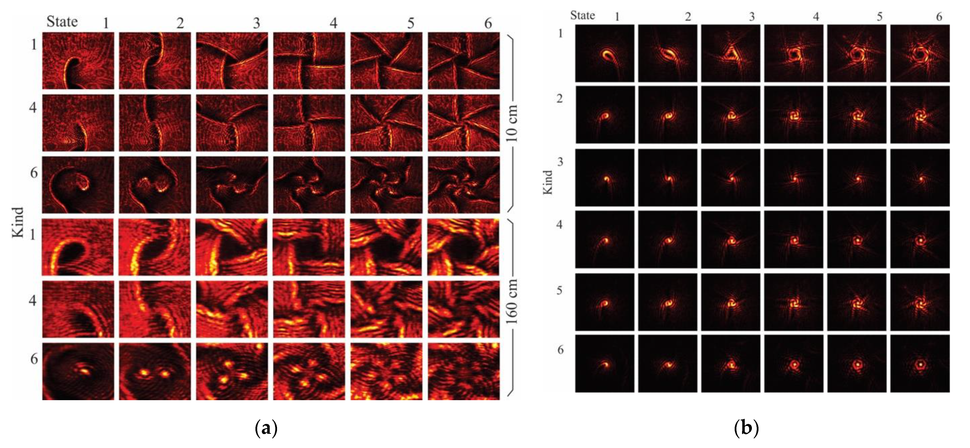
Following the SLM, the beam was relayed with a 4-f lens system and only the first diffraction order was allowed to pass the spatial filter F1. The CCD camera images the conjugate plane (CP) of the SLM. For a short-path configuration, mirrors M2 to M4 were removed, leaving a propagation path of 10 cm. An extended experimental path of approximately 160 cm—using mirrors M2 to M4—was included to study the development of the beams, which were expected to evolve due to their non-modal characteristics. The resulting beam profiles for both propagation distances are shown in Figure 5a.
A second experiment was performed with which the beams could propagate over a longer distance through a focused telescope. A schematic of the experiment is shown in Figure 4b. With this setup we were able to observe more developed beam patterns, where we could observe how the intensity evolved from the uniformly illuminated wave to the actual beam. Recordings of the intensity profiles are depicted on Figure 5b. A third experiment was performed to observe the far field at the focus using a single-lens configuration, as shown in Figure 4c. By changing the phase curvature at the SLM we could observe the beam profile before and after the focus. These results are shown in Figure 6, images (a) through (e).
4. Results and Discussion
4.1. Analysis
A comparison of the different Kinds from Figure 2, Figure 3 and Figure 5a reveals that there was a very good correspondence between theoretical singular beams and experimental realizations. Another interesting characteristic that can be observed in those figures is that odd radial functions—linear, cubic, and tangential—produced a warp that turned counterclockwise, while the quadratic profile created clockwise turns. Kinds 4 and 5 have a sine and cosine function and neither of them produce a negative phase at the origin; that is why they produced a clockwise turn even though one was odd, and the other was even. In the experimental intensity profiles, the observed rotations confirmed the simulated results, although there is a vertical flip due to the lens system. Comparing the images on Figure 5a,b, it appears that Kind 1 was the only beam that retained a central dark spot. Beams of this Kind had several dark spots that suggested they carried a central singularity like a Laguerre–Gaussian beam. On every other Kind, it is clear that the singularity of each state was displaced from the central position. Finally, the tangent radial profile created interesting fan-like beams, that were difficult to predict. Nevertheless, for longer propagation they were not different from other trigonometric Kinds like 4 and 5. This can be seen in Figure 5b.
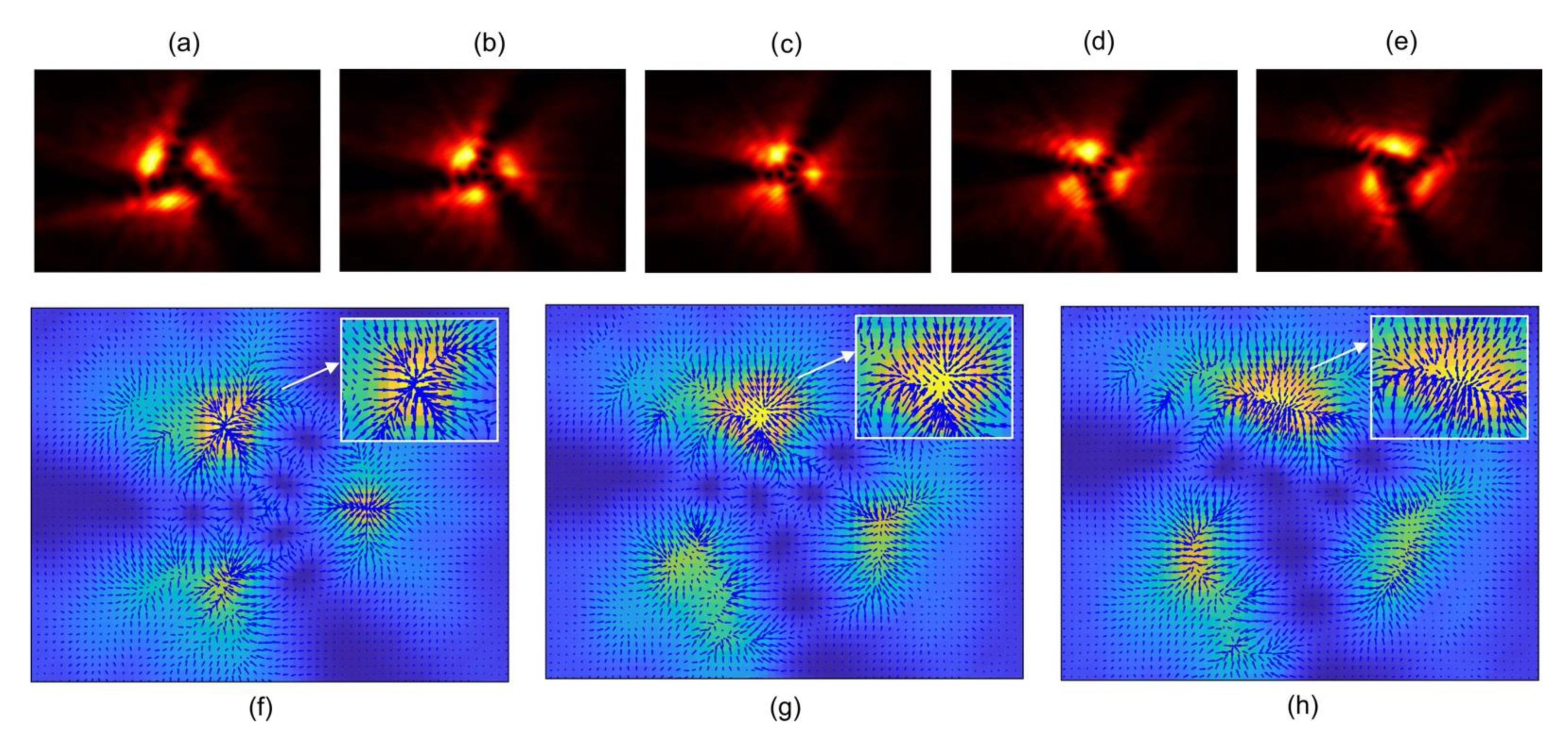
A group of selected results of the third experiment (See Figure 4c) are shown in Figure 6, where we have selected for analysis. In this case, image (c) corresponds to the focal point while (a) and (b) represent the beam shape before focus and (d) and (e) show the beam after focus. Figure 6a must be compared with Figure 5b , that retained the same triangular form. Within the focal range it can be seen that the singularities were located in a starlike configuration, reminiscent of the phase pattern that generated this beam (See Figure 2).
4.2. Application
Optical tweezers require a focused image of the trapping beam, that is, the far field image or Fraunhofer diffraction pattern. In this case instead of using a direct Gaussian beam it is possible to use a singular beam by applying an SLM device [30]. If the SLM was programmed to create a tangent beam, then it could be converted to an optical tweezer. Tangent beams provided different kind of modulations aside from the TC, for example the variable y0 (See Equation (1)) could change the turning point towards the center of the beam. In a non-static scenario, it was possible to obtain a dynamic translocation that might be useful for radial particle displacement. The intensity gradient could provide the optical force necessary to implement a particle trapping. In theory it could be used as a general qualitative technique for these kinds of beams. The method followed the characterization of lateral gradient intensities. As mentioned earlier, the beams must be in the focus region of a microscope objective (for example 60× or 0.9 NA) to convert them into an optical trapping region. According to Neumann and Block, effective trapping occurs when the gradient force overcomes the scattering one [22], the first is proportional to the intensity gradient value and the second to the mean intensity. Then, if the ratio of intensity gradient value to mean intensity value of a region of interest of a beam exceed the unit (∇I/⟨I⟩ > 1), thus lead to consider it as suitable region for trapping. In this case we were not able to measure the axial intensity gradient, but we could provide the transverse intensity gradient sufficient to get a qualitative conclusion.
In Figure 6, we present some examples of some results obtained from setup 3 for the analysis. An intensity image gradient was performed to exhibit the gradient vector field. Those were obtained by the gradient of the intensity values per pixel. Aside from considering the central maximum, we were interested to know more about the peripheral regions of the beams, since they could be modulated by changing parameters like α or y0. Figure 6f,g,h shown the transverse intensity gradient field of images (c), (d) and (e). The high intensity regions could offer good conditions for optical trapping. In this case the direction of the arrows was appropriate for trapping particles that were attracted to light, that is, when the particle refractive index was greater than the refractive index of the medium [22]. Figure 6 also shows a zoomed area of an optical convergent region. In general aspects, the modes exhibited promising conditions for optical manipulation. Since the camera resolution was 2.5 μm per pixel size our actual setup could virtually move particles of approximately this size or larger. However, according to [30] with a similar configuration they can observe trapping of 2 μm particles using a 7 μm camera pixel size. For particles that have a refractive index lower than the surrounding medium, the dark spots can also be converted to trapping regions [31]. In this case by observing Figure 6f,g,h, there were at least six singular dark points that were rotating around the center while the beam passed through the focal point.
5. Conclusions
We have successfully created several new laser beam profiles based on simple mathematical functions. These functions, when used as a phase pattern, can generate beams exhibiting peculiar intensity profiles whose characteristics are inherited from their radial function. The non-periodic functions have one turning point, that represents a phase discontinuity, while the periodic ones manifest several discontinuities, depending on the period. We have seen that for the choice of fixed turning point (y0 or x0) is best to keep the intensity twist within the extent of the beam. This choice is arbitrary and depends on the diffracting device used. If the turning point is variable (dependent of l) the radial twists could turn towards or away the center as l increases. The modification of the multiplier α results in a great change in the shape of the beam. Even though we used a fixed value for our experiments and simulations, the possibility of changing this value dynamically opens new possibilities. Moreover, with the intensity gradient map provided, we present these beams as a good candidate for optical tweezers.
Author Contributions
Conceptualization, G.F.; methodology, G.F.; software, G.F.; validation, G.F., E.P. and J.A.; formal analysis, G.F. and E.P.; investigation, G.F.; resources, J.A.; data curation, G.F.; writing—original draft preparation, G.F.; writing—review and editing, G.F., E.P. and J.A.; visualization, G.F.; supervision, J.A.; project administration, J.A.; funding acquisition, J.A. All authors have read and agreed to the published version of the manuscript.
Funding
This work has been funded in part by CONICYT under grant FR-1160887 and FI-11160146, and by the Millennium Institute for Research in Optics (MIRO), Chile.
Informed Consent Statement
Not applicable.
Data Availability Statement
Not applicable.
Acknowledgments
The authors would like to thank Juan Staforelli for his assistance in the application section.
Conflicts of Interest
The authors declare no conflict of interest.
References
- Rubinsztein-Dunlop, H.; Forbes, A.; Berry, M.V.; Dennis, M.R.; Andrews, D.L.; Mansuripur, M.; Denz, C.; Alpmann, C.; Banzer, P.; Bauer, T.; et al. A Roadmap to structured light. J. Opt. 2016, 19, 013001. [Google Scholar] [CrossRef]
- Lamperska, W.; Masajada, J.; Drobczyński, S.; Wasylczyk, P. Optical vortex torque measured with optically trapped microbarbells. Appl. Opt. 2020, 59, 4703–4707. [Google Scholar] [CrossRef] [PubMed]
- Gahagan, K.T.; Swartzlander, G. Optical vortex trapping of particles. Opt. Lett. 1996, 21, 827–829. [Google Scholar] [CrossRef] [PubMed]
- Tian, Y.; Wang, L.; Duan, G.; Yu, L. Multi-trap optical tweezers based on composite vortex beams. Opt. Commun. 2021, 485, 126712. [Google Scholar] [CrossRef]
- Palacios, D.; Rozas, D.; Swartzlander, J.G.A. Observed Scattering into a Dark Optical Vortex Core. Phys. Rev. Lett. 2002, 88, 103902. [Google Scholar] [CrossRef] [Green Version]
- Li, L.; Song, H.; Zhang, R.; Zhao, Z.; Liu, C.; Pang, K.; Song, H.; Du, J.; Willner, A.N.; Almaiman, A.; et al. Increasing system tolerance to turbulence in a 100-Gbit/s QPSK free-space optical link using both mode and space diversity. Opt. Commun. 2021, 480, 126488. [Google Scholar] [CrossRef]
- Davis, J.A.; Cottrell, D.M.; Campos, J.; Yzuel, M.; Moreno, I. Encoding amplitude information onto phase-only filters. Appl. Opt. 1999, 38, 5004–5013. [Google Scholar] [CrossRef]
- Meltaus, J.; Salo, J.; Noponen, E.; Salomaa, M.; Viikari, V.; Lonnqvist, A.; Koskinen, T.; Saily, J.; Hakli, J.; Ala-Laurinaho, J.; et al. Millimeter-wave beam shaping using holograms. IEEE Trans. Microw. Theory Tech. 2003, 51, 1274–1280. [Google Scholar] [CrossRef]
- Bekshaev, A.; Karamoch, A. Spatial characteristics of vortex light beams produced by diffraction gratings with embedded phase singularity. Opt. Commun. 2008, 281, 1366–1374. [Google Scholar] [CrossRef]
- Lóxpez-Mariscal, C.; Gutiérrez-Vega, J.C.; Milne, G.; Dholakia, K. Orbital angular momentum transfer in helical Mathieu beams. Opt. Express 2006, 14, 4182–4187. [Google Scholar] [CrossRef]
- Hernández-Hernández, R.J.; Terborg, R.A.; Ricardez-Vargas, I.; Volke-Sepúlveda, K. Experimental generation of Mathieu-Gauss beams with a phase-only spatial light modulator. Appl. Opt. 2010, 49, 6903–6909. [Google Scholar] [CrossRef]
- Alonzo, C.A.; Rodrigo, P.J.; Glückstad, J. Helico-conical optical beams: A product of helical and conical phase fronts. Opt. Express 2005, 13, 1749–1760. [Google Scholar] [CrossRef] [Green Version]
- Lee, S.-H.; Roichman, Y.; Grier, D. Optical solenoid beams. Opt. Express 2010, 18, 6988–6993. [Google Scholar] [CrossRef] [Green Version]
- Daria, V.R.; Palima, D.Z.; Glückstad, J. Optical twists in phase and amplitude. Opt. Express 2011, 19, 476–481. [Google Scholar] [CrossRef] [Green Version]
- MacDonald, M.; Volke-Sepulveda, K.; Paterson, L.; Arlt, J.; Sibbett, W.; Dholakia, K. Revolving interference patterns for the rotation of optically trapped particles. Opt. Commun. 2002, 201, 21–28. [Google Scholar] [CrossRef]
- Zhang, P.; Huang, S.; Hu, Y.; Hernandez, D.; Chen, Z. Generation and nonlinear self-trapping of optical propelling beams. Opt. Lett. 2010, 35, 3129–3131. [Google Scholar] [CrossRef]
- Sui, X.; Zhao, J.; Liu, B.; Yan, Z.; Cao, C.; Zhou, S. Self-acceerating fan-shaped beams along arbitrary trajectories: A new tool for optical manipulation. J. Opt. 2016, 19, 015611. [Google Scholar] [CrossRef]
- Lu, Z.; Yan, B.; Chang, K.; Qiao, Y.; Li, C.; Hu, J.; Xu, T.; Zhang, H.; Lin, W.; Yue, Y.; et al. Space division multiplexing technology based on transverse wavenumber of Lommel–Gaussian beam. Opt. Commun. 2021, 488, 126835. [Google Scholar] [CrossRef]
- Ashkin, A. Acceleration and Trapping of Particles by Radiation Pressure. Phys. Rev. Lett. 1970, 24, 156–159. [Google Scholar] [CrossRef] [Green Version]
- Ashkin, A.; Dziedzic, J.M.; Bjorkholm, J.E.; Chu, S. Observation of a single-beam gradient force optical trap for dielectric particles. Opt. Lett. 1986, 11, 288–290. [Google Scholar] [CrossRef] [PubMed] [Green Version]
- Ashkin, A. Optical trapping and manipulation of neutral particles using lasers. Proc. Natl. Acad. Sci. USA 1997, 94, 4853–4860. [Google Scholar] [CrossRef] [Green Version]
- Neuman, K.; Block, S.M. Optical trapping. Rev. Sci. Instrum. 2004, 75, 2787–2809. [Google Scholar] [CrossRef]
- Moffitt, J.R.; Chemla, Y.R.; Smith, S.B.; Bustamante, C. Recent advances in optical tweezers. Annu. Rev. Biochem. 2008, 77, 205–228. [Google Scholar] [CrossRef] [Green Version]
- Friese, M.E.J.; Enger, J.; Rubinsztein-Dunlop, H.; Heckenberg, N.R. Optical angular-momentum transfer to trapped absorbing particles. Phys. Rev. A 1996, 54, 1593–1596. [Google Scholar] [CrossRef] [Green Version]
- Bustamante, C. Of torques, forces, and protein machines. Protein Sci. 2009, 13, 3061–3065. [Google Scholar] [CrossRef]
- Parkin, S.J.; Vogel, R.; Persson, M.; Funk, M.; Loke, V.L.Y.; Nieminen, T.A.; Heckenberg, N.R.; Rubinsztein-Dunlop, H. Highly birefringent vaterite microspheres: Production, characterization and applications for optical micromanipulation. Opt. Express 2009, 17, 21944–21955. [Google Scholar] [CrossRef]
- Peters, E.; Funes, G.; Anguita, J.A. Singular beams based on tangential phase warp. Opt. Lett. 2019, 44, 3769–3772. [Google Scholar] [CrossRef] [PubMed]
- He, H.; Heckenberg, N.; Rubinsztein-Dunlop, H. Optical Particle Trapping with Higher-order Doughnut Beams Produced Using High Efficiency Computer Generated Holograms. J. Mod. Opt. 1995, 42, 217–223. [Google Scholar] [CrossRef]
- Anguita, J.A.; Herreros, J.; Djordjevic, I.B. Coherent multimode OAM superpositions for multidimensional modulation. IEEE Photon. J. 2014, 6, 1–11. [Google Scholar] [CrossRef]
- Cojoc, D.; Garbin, V.; Ferrari, E.; Businaro, L.; Romanato, F.; Di Fabrizio, E. Laser trapping and micro-manipulation using optical vortices. Microelectron. Eng. 2005, 78, 125–131. [Google Scholar] [CrossRef]
- Melo, B.; Brandão, I.; Da, B.S.P.; Rodrigues, R.; Khoury, A.; Guerreiro, T. Optical trapping in a dark focus. Phys. Rev. Appl. 2020, 14, 034069. [Google Scholar] [CrossRef]
Figure 1.
Example of a wavefront with warped profiles according to Equation (1). The blue lines represent the tangential profile while the dotted curve represents the turning point.
Figure 1.
Example of a wavefront with warped profiles according to Equation (1). The blue lines represent the tangential profile while the dotted curve represents the turning point.
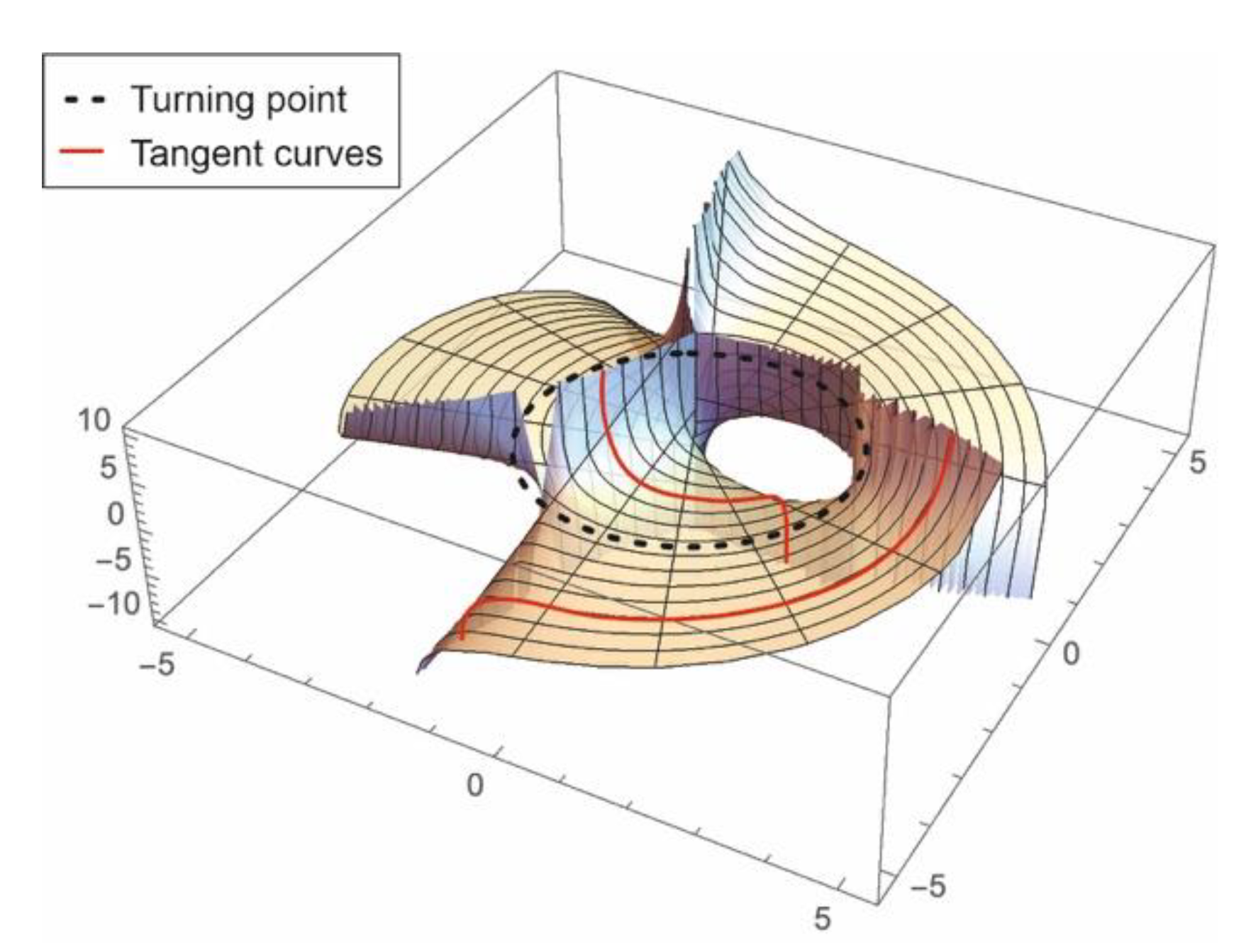
Figure 2.
Columns 1 to 3: examples of phase patterns for the generation of singular beams. Each Kind is evaluated for states to . Columns 4 to 6: intensity profiles as generated from the phase patterns in columns 1 to 3, for a propagation of 62 cm. Each Kind is evaluated for states to .
Figure 2.
Columns 1 to 3: examples of phase patterns for the generation of singular beams. Each Kind is evaluated for states to . Columns 4 to 6: intensity profiles as generated from the phase patterns in columns 1 to 3, for a propagation of 62 cm. Each Kind is evaluated for states to .
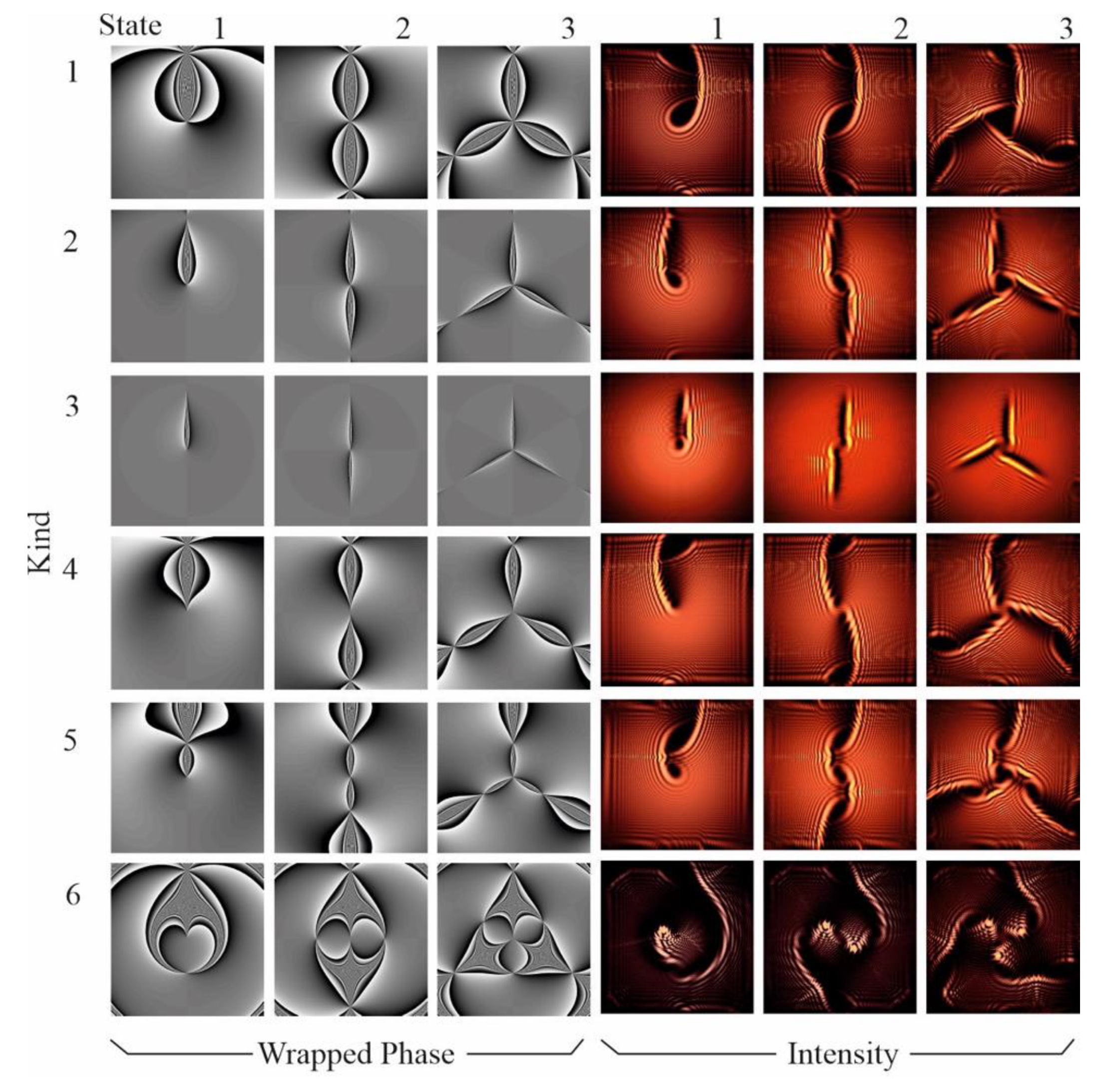
Figure 3.
Simulated intensity profiles of Kind-3 beams propagated at distances 0.01, 0.3, 1, 1.6, and 2 m, for states through 6.
Figure 3.
Simulated intensity profiles of Kind-3 beams propagated at distances 0.01, 0.3, 1, 1.6, and 2 m, for states through 6.
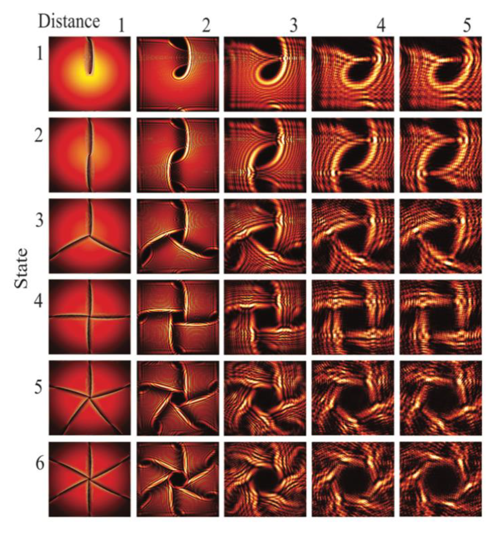
Figure 4.
(a) Experimental setup. (Setup 1) (L) pigtailed 633 nm laser source, (P) linear polarizer, (E) beam expander, (BSC) beam-splitter cube, (SLM) reflection spatial light modulator, (M1, M2, M3 M4) mirrors, (L1, L2) 150 mm lenses, (F1, F2) filters, (CP) conjugate plane, (L3) 100 mm lens, (CCD) camera. This diagram exhibits the long path configuration. To achieve the shortest path, mirrors M2, M3 and M4 are removed. (b) (Setup 2) Experimental setup for long propagation. The difference from Setup 1 is the Keplerian beam expanders and the propagation over a 4 m path. The second expander collects the beam that passes through a series of mirrors to ensure a far field image. Finally, a full HD camera (HDC) is used to record the images. (c) (Setup 3) (L) HeNe laser source, (NDF) neutral density filter (BSC) beam-splitter cube, (SLM) reflection spatial-light modulator, (M1) mirror, (L1) 400 mm lens, (F1) filter, (CCD) camera.
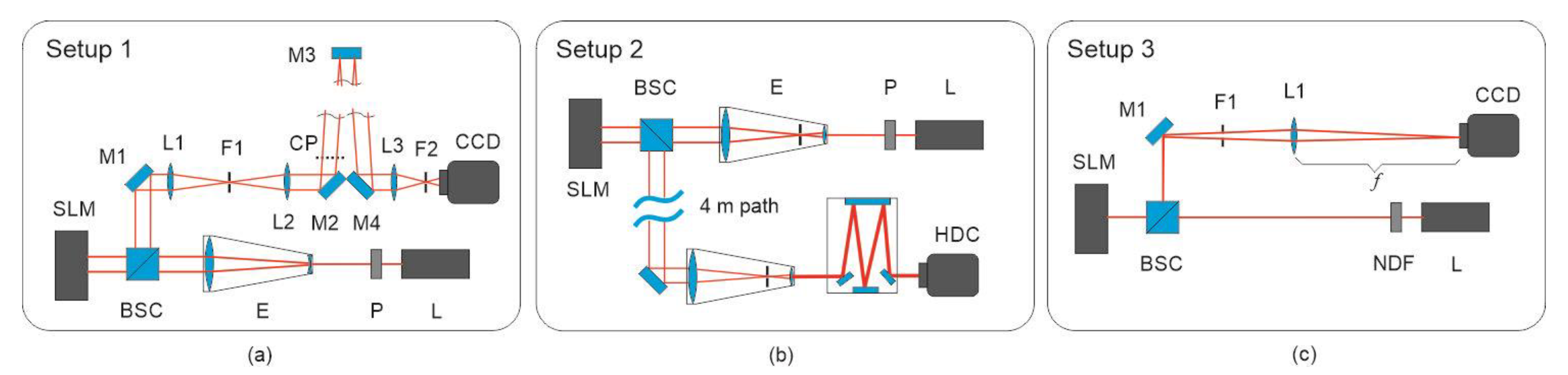
Figure 5.
(a) Propagation of Kinds 1, 4 and 6 at distances 10 and 160 cm, and states = 1 to 6. (b) Images obtained from Setup 2 (Figure 4b). Figure shows the propagation of all Kinds and states = 1 to 6 for longer propagation.
Figure 5.
(a) Propagation of Kinds 1, 4 and 6 at distances 10 and 160 cm, and states = 1 to 6. (b) Images obtained from Setup 2 (Figure 4b). Figure shows the propagation of all Kinds and states = 1 to 6 for longer propagation.

Figure 6.
(a–e) Far field images of obtained from the experimental setup 3. (a,b) corresponds to 4 and 2 inches before the focus, respectively. (c) is the focus image, while (d,e) represents the image 2 and 4 inches post focus. (f) intensity gradient of image (c) and an example of zoomed region. (g) intensity gradient of image (d). (h) intensity gradient of image (e).
Publisher’s Note: MDPI stays neutral with regard to jurisdictional claims in published maps and institutional affiliations. |
© 2021 by the authors. Licensee MDPI, Basel, Switzerland. This article is an open access article distributed under the terms and conditions of the Creative Commons Attribution (CC BY) license (https://creativecommons.org/licenses/by/4.0/).
Share and Cite
MDPI and ACS Style
Funes, G.; Peters, E.; Anguita, J. Singular Warped Beams Controlled by Tangent Phase Modulation. Photonics 2021, 8, 343. https://doi.org/10.3390/photonics8080343
AMA Style
Funes G, Peters E, Anguita J. Singular Warped Beams Controlled by Tangent Phase Modulation. Photonics. 2021; 8(8):343. https://doi.org/10.3390/photonics8080343
Chicago/Turabian StyleFunes, Gustavo, Eduardo Peters, and Jaime Anguita. 2021. "Singular Warped Beams Controlled by Tangent Phase Modulation" Photonics 8, no. 8: 343. https://doi.org/10.3390/photonics8080343
Note that from the first issue of 2016, this journal uses article numbers instead of page numbers. See further details here.