Measurement of Focal Length and Radius of Curvature for Spherical Lenses and Mirrors by Using Digital-Grating Moiré Effect


 ,
, 

Abstract
:1. Introduction
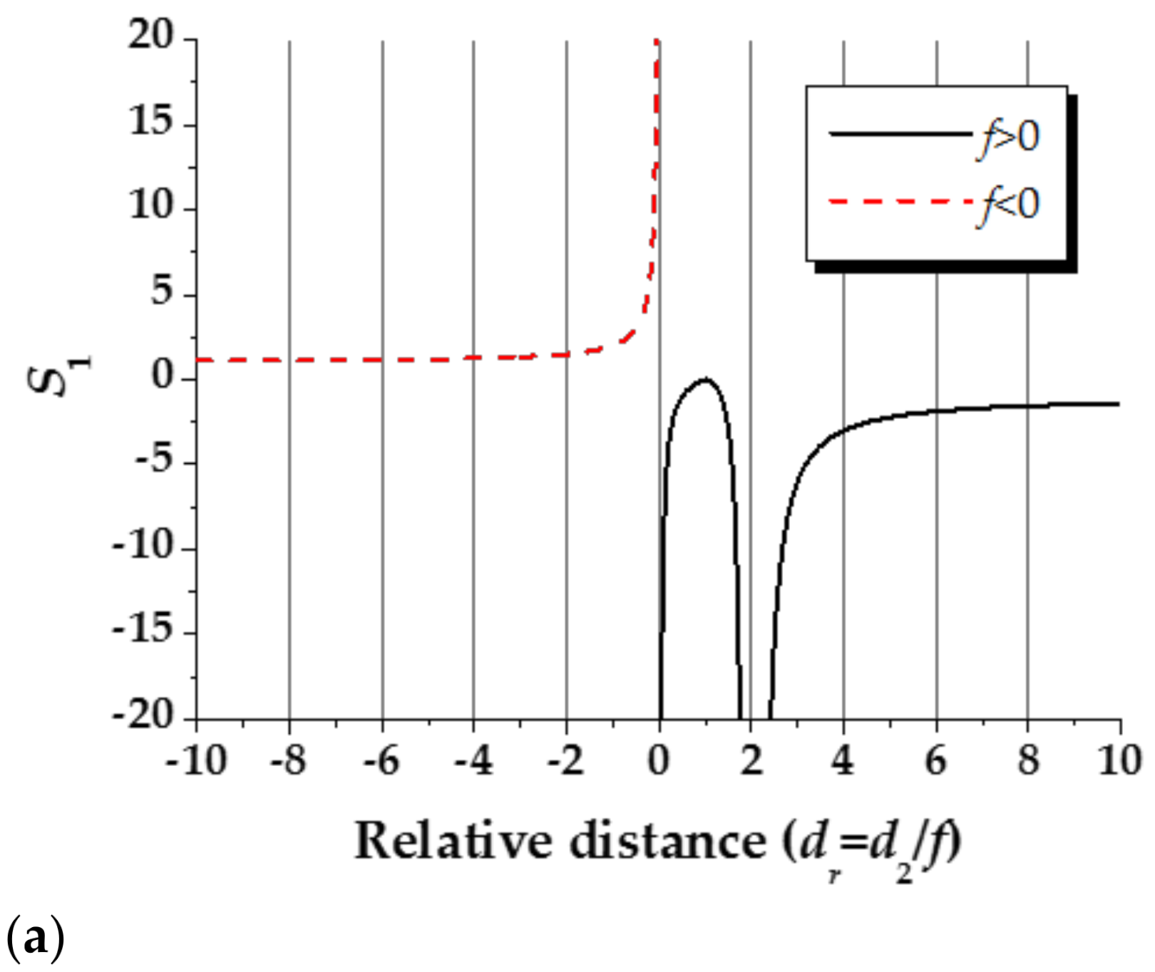
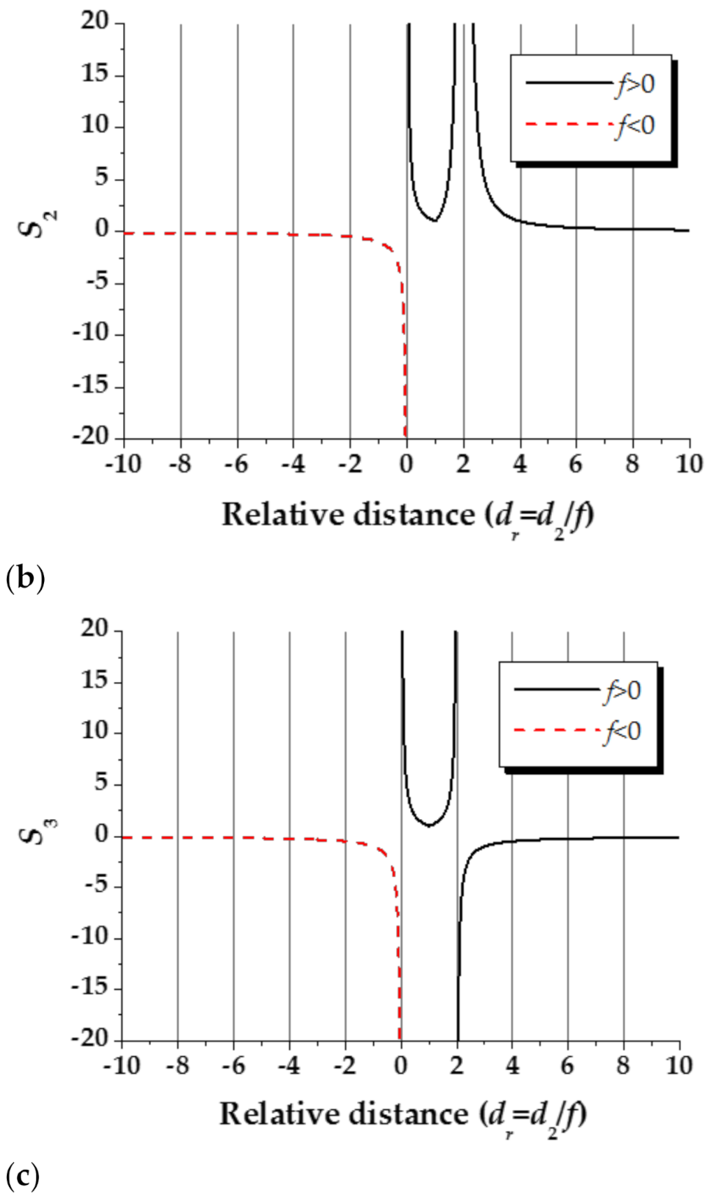
2. Principles
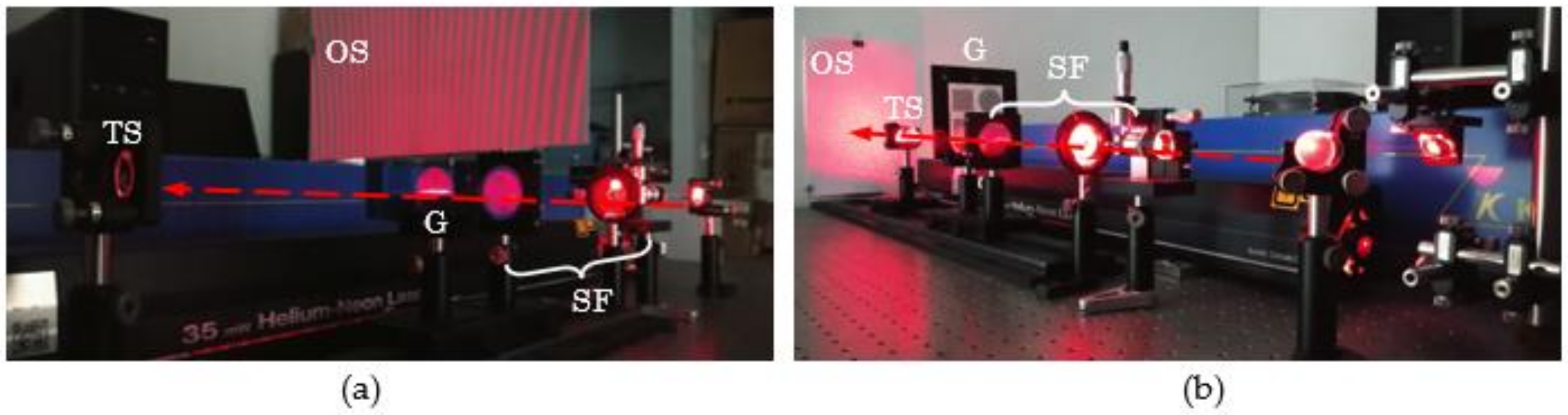
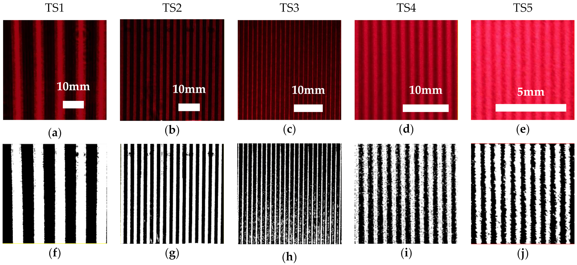
3. Experimental Results and Discussion
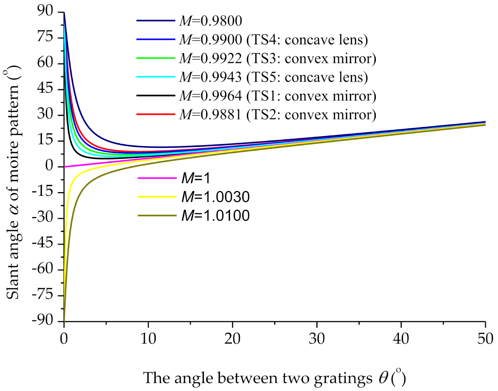
3.1. Determination of the Slant Angle for the Digital Gratings
3.2. Analysis of Measurement Uncertainty
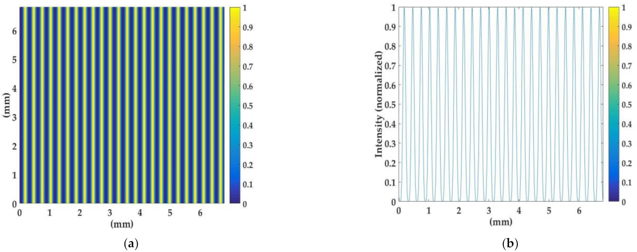
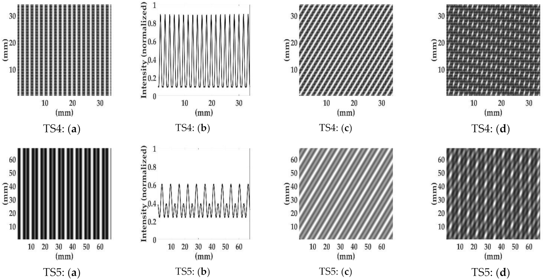
3.3. Simulation of Light Field Distributions
4. Conclusions
Author Contributions
Funding
Institutional Review Board Statement
Informed Consent Statement
Acknowledgments
Conflicts of Interest
Appendix A

| dr = d2/f | ||||||||||||
|---|---|---|---|---|---|---|---|---|---|---|---|---|
| 2.5 | 5 | 10 | 20 | 30 | 40 | |||||||
| f | p1 0.282 | p1 1.00 | p1 0.282 | p1 1.00 | p1 0.282 | p1 1.00 | p1 0.282 | p1 1.00 | p1 0.282 | p1 1.00 | p1 0.282 | p1 1.00 |
| 10 | 3.7 | 1.3 | 0.2 | 0.1 | 0.1 | 0.1 | 0.1 | 0.1 | 0.1 | 0.1 | 0.1 | 0.1 |
| −10 | 0.2 | 0.1 | 0.1 | 0.1 | 0.1 | 0.1 | 0.1 | 0.1 | 0.1 | 0.1 | 0.1 | 0.1 |
| 25 | 9.2 | 3.2 | 0.6 | 0.3 | 0.3 | 0.2 | 0.2 | 0.2 | 0.2 | 0.2 | 0.2 | 0.1 |
| −25 | 0.4 | 0.2 | 0.3 | 0.2 | 0.2 | 0.2 | 0.2 | 0.1 | 0.2 | 0.1 | 0.2 | 0.1 |
| 50 | 18.4 | 6.5 | 1.2 | 0.7 | 0.5 | 0.4 | 0.4 | 0.3 | 0.4 | 0.3 | 0.4 | 0.3 |
| −50 | 0.8 | 0.4 | 0.5 | 0.3 | 0.4 | 0.3 | 0.3 | 0.3 | 0.3 | 0.3 | 0.3 | 0.3 |
| 100 | 36.7 | 12.9 | 2.4 | 1.3 | 1.1 | 0.8 | 0.8 | 0.6 | 0.7 | 0.6 | 0.7 | 0.6 |
| −100 | 1.7 | 0.9 | 1.0 | 0.7 | 0.8 | 0.6 | 0.7 | 0.6 | 0.7 | 0.6 | 0.7 | 0.6 |
| 150 | 55.1 | 19.4 | 3.6 | 2.0 | 1.6 | 1.2 | 1.2 | 1.0 | 1.1 | 0.9 | 1.1 | 0.9 |
| −150 | 2.5 | 1.3 | 1.6 | 1.0 | 1.2 | 0.9 | 1.0 | 0.9 | 1.0 | 0.8 | 1.0 | 0.8 |
| 200 | 73.5 | 25.8 | 4.9 | 2.7 | 2.1 | 1.6 | 1.6 | 1.3 | 1.5 | 1.2 | 1.4 | 1.2 |
| −200 | 3.4 | 1.7 | 2.1 | 1.4 | 1.6 | 1.2 | 1.4 | 1.1 | 1.3 | 1.1 | 1.3 | 1.1 |
References
- Kingslake, R. Applied Optics and Optical Engineering; Academic Press: New York, NY, USA; Volume I, pp. 208–226.
- Luo, J.; Bai, J.; Zhang, J.; Hou, C.; Wang, K.; Hou, X. Long focal-length measurement using divergent beam and two gratings of different periods. Opt. Express 2014, 22, 27921–27931. [Google Scholar] [CrossRef] [PubMed]
- Jin, X.; Zhang, J.; Bai, J.; Hou, C.; Hou, X. Calibration method for high-accuracy measurement of long focal length with Talbot interferometry. Appl. Opt. 2012, 51, 2407–2413. [Google Scholar] [CrossRef] [PubMed]
- Chen, J.-H.; Chen, K.-H.; Han, C.-Y.; Wu, C.-W.; Wu, N.-Y. Evaluation of the curvature of an object by Talbot interferometry. Opt. Rev. 2009, 16, 489–491. [Google Scholar] [CrossRef]
- KSriram, K.V.; Kothiyal, M.P.; Sirohi, R.S. Talbot interferometry in noncollimated illumination for curvature and focal length measurements. Appl. Opt. 1992, 31, 75–79. [Google Scholar] [CrossRef] [PubMed]
- Bernardo, L.M.; Soares, O.D.D. Evaluation of the focal distance of a lens by Talbot interferometry. Appl. Opt. 1988, 27, 296–301. [Google Scholar] [CrossRef]
- Arriaga-Hernández, J.A.; Jaramillo-Núñez, A. Ronchi and Moiré patterns for testing spherical and aspherical surfaces using deflectometry. Appl. Opt. 2018, 57, 9963–9971. [Google Scholar] [CrossRef]
- Hong, T.; Li, D.; Wang, R.; Zhang, X.; Liu, X. Method for measuring the radius of mean curvature of a spherical surface based on phase measuring deflectometry. Appl. Opt. 2021, 60, 1705–1709. [Google Scholar] [CrossRef] [PubMed]
- Singh, P.; Faridi, M.S.; Shakher, C.; Sirohi, R.S. Measurement of focal length with phase-shifting Talbot interferometry. Appl. Opt. 2005, 44, 1572–1576. [Google Scholar] [CrossRef] [PubMed]
- De Nicola, S.; Ferraro, P.; Finizio, A.; Pierattini, G. Reflective grating interferometer for measuring the focal length of a lens by digital moiré effect. Opt. Commun. 1996, 132, 432–436. [Google Scholar] [CrossRef]
- De Angelis, M.; De Nicola, S.; Ferraro, P.; Finizio, A.; Pierattini, G. Analysis of moiré fringes for measuring the focal length of lenses. Opt. Lasers Eng. 1998, 30, 279–286. [Google Scholar] [CrossRef]
- Lee, S. Talbot Interferometry for Measuring the Focal Length of a Lens without Moiré Fringes. J. Opt. Soc. Korea 2015, 19, 165–168. [Google Scholar] [CrossRef] [Green Version]
- Goodman, J.W. Introduction to Fourier Optics, 3rd ed.; W. H. Freeman: Englewood, CO, USA, 2004. [Google Scholar]
- Gåsvik, K.J. Optical Metrology; Wiley: Hoboken, NJ, USA, 1987. [Google Scholar]


| Test Samples | Angle θ (°) | Slant Angle α (°) | Experimental Value of Focal Length (mm) | Reference Value of Focal Length (mm) | Percent Error (%) |
|---|---|---|---|---|---|
| Experimental Value of Radius of Curvature (mm) | Reference Value of Radius of Curvature (mm) | Percent Error (%) | |||
| TS1 | 30.00 | 15.46 | −7.757 | −7.751 | 0.0774 |
| −15.51 | −15.50 | 0.0645 | |||
| TS2 | 30.00 | 15.35 | −25.67 | −25.80 | 0.5039 |
| −51.34 | −51.60 | 0.5039 | |||
| TS3 | 30.00 | 15.79 | −52.05 | −52.08 | 0.0576 |
| −104.1 | −104.2 | 0.0960 | |||
| TS4 | 30.00 | 15.83 | −49.85 | −50.00 | 0.3000 |
| −51.36 (R1) | −51.51 (R1) | 0.2912 | |||
| TS5 | 30.00 | 15.50 | −199.6 | −200.0 | 0.2000 |
| −205.6 (R1) | −206.0 (R1) | 0.1942 |
| Test Samples | |||||||||||
|---|---|---|---|---|---|---|---|---|---|---|---|
| TS1 | 0.1417 | 0.282 0.005 | 0.0236 | 9.480 0.028 | 0.0092 | 251.7 0.3 | 0.1414 | 15.46 0.03 | 0.0684 | 0.03 | 0.2 |
| TS2 | 0.4987 | 0.282 0.005 | 0.2565 | 3.072 0.028 | 0.0305 | 251.7 0.3 | 0.4978 | 15.35 0.03 | 0.2428 | 0.03 | 0.8 |
| TS3 | 1.1130 | 0.282 0.005 | 1.0602 | 1.659 0.028 | 0.0620 | 251.7 0.3 | 1.1111 | 15.79 0.03 | 0.5249 | 0.03 | 2.0 |
| TS4 | 1.0585 | 0.282 0.005 | 0.9725 | 1.720 0.028 | 0.0594 | 251.7 0.3 | 1.0567 | 15.83 0.03 | 0.4978 | 0.03 | 1.9 |
| TS5 | 6.3423 | 0.282 0.005 | 15.6363 | 0.641 0.028 | 0.2379 | 251.7 0.3 | 6.3309 | 15.50 0.03 | 3.0550 | 0.03 | 18.3 |
Publisher’s Note: MDPI stays neutral with regard to jurisdictional claims in published maps and institutional affiliations. |
© 2021 by the authors. Licensee MDPI, Basel, Switzerland. This article is an open access article distributed under the terms and conditions of the Creative Commons Attribution (CC BY) license (https://creativecommons.org/licenses/by/4.0/).
Share and Cite
Han, C.-Y.; Lo, W.-T.; Chen, K.-H.; Lee, J.-Y.; Yeh, C.-H.; Chen, J.-H. Measurement of Focal Length and Radius of Curvature for Spherical Lenses and Mirrors by Using Digital-Grating Moiré Effect. Photonics 2021, 8, 252. https://doi.org/10.3390/photonics8070252
Han C-Y, Lo W-T, Chen K-H, Lee J-Y, Yeh C-H, Chen J-H. Measurement of Focal Length and Radius of Curvature for Spherical Lenses and Mirrors by Using Digital-Grating Moiré Effect. Photonics. 2021; 8(7):252. https://doi.org/10.3390/photonics8070252
Chicago/Turabian StyleHan, Chien-Yuan, Wen-Tai Lo, Kun-Huang Chen, Ju-Yi Lee, Chien-Hung Yeh, and Jing-Heng Chen. 2021. "Measurement of Focal Length and Radius of Curvature for Spherical Lenses and Mirrors by Using Digital-Grating Moiré Effect" Photonics 8, no. 7: 252. https://doi.org/10.3390/photonics8070252
APA StyleHan, C.-Y., Lo, W.-T., Chen, K.-H., Lee, J.-Y., Yeh, C.-H., & Chen, J.-H. (2021). Measurement of Focal Length and Radius of Curvature for Spherical Lenses and Mirrors by Using Digital-Grating Moiré Effect. Photonics, 8(7), 252. https://doi.org/10.3390/photonics8070252