Image Processing for Laser Imaging Using Adaptive Homomorphic Filtering and Total Variation

Abstract

Laser active imaging technology has important practical value and broad application prospects in military fields such as target detection, radar reconnaissance, and precise guidance. However, factors such as uneven laser illuminance, atmospheric backscatter, and the imaging system itself will introduce noise, which will affect the quality of the laser active imaging image, resulting in image contrast decline and blurring image edges and details. Therefore, an image denoising algorithm based on homomorphic filtering and total variation cascade is proposed in this paper, which strives to reduce the noise while retaining the edge features of the image to the maximum extent. Firstly, the image type is determined according to the characteristics of the laser image, and then the speckle noise in the low-frequency region is suppressed by adaptive homomorphic filtering. Finally, the image denoising method of minimizing the total variation is adopted for the impulse noise and Gaussian noise. Experimental results show that compared with separate homomorphic filtering, total variation filtering, and median filtering, the proposed algorithm significantly improves the contrast, retains edge details, achieves the expected effect. It can better adjust the image brightness and is beneficial for subsequent processing.

1. Introduction

The sensitivity of intensified charge-coupled devices (ICCDs), atmospheric turbulence, laser energy, structural characteristics of the receiving optical system, and non-uniformity of the illumination will all affect the quality of a laser image. If the imaging conditions are poor, the signal-to-noise ratio of the obtained laser image will be reduced, and the contrast and brightness will become worse, which will cause great difficulties to image recognition. In addition to the influence of background light, the noise caused by the laser active imaging system is also a major factor affecting the characteristics of the laser image. In the process of acquiring an image by a laser active imaging system, various electronic noises of the optical system, the system, and the speckle noise of the laser will affect the resulting image.

Various types of noise were finally introduced into the final imaging and manifested in three main forms of noise: impulse noise [1,2,3], Gaussian noise, and speckle noise [4,5]. Many scholars have performed in-depth studies on the problem of the restoration of images contaminated by noise, as in [1], where a weighted couple sparse representation model is presented to remove impulse noise. The dictionary is directly trained on the noisy raw data by addressing a weighted rank-one minimization problem, which can capture more features of the original data. In [2], a new TV-MCP model and its proximation method are proposed. The maximum SNR can reach two times that of the TVL1 method. In [3], a novel model that uses a devised cost function involving semi-supervised learning based on a large amount of corrupted image data with a few labeled training samples is proposed. In addition, speckle noise is one of the characteristics of laser image that is different from visible images. The previous literature is usually directed to a certain kind of noise. There are three kinds of noise in the laser image at the same time. It is difficult to determine which one has the greater impact. We must comprehensively consider the characteristics of each noise. A suitable filter must be selected to eliminate various noises according to the advantages and disadvantages of various types of filters. Most of the speckle noise in the laser image is concentrated in the low-frequency region, hence the homomorphic filtering is selected to suppress the low-frequency part. After high pass filtering, the low-frequency part is reduced and the high-frequency part is enhanced, so as to remove the speckle noise and improve the contrast of the image; for impulse noise and Gaussian noise, image denoising method with total variation minimization is used, and the edge features of the image are preserved to the maximum during noise reduction. The process of the proposed algorithm is as follows: firstly, the image is homomorphically filtered, the image contrast is improved, the speckle noise of the laser image is removed, and then a total variation minimization model is adopted to remove Gaussian noise and impulse noise of the laser image. In the selection of homomorphic filtering parameters, the c value has a great influence for different images. In general, the laser should irradiate the target, and the target itself corresponds to the pixel with larger brightness. During night imaging, the brightness of the background around the target is very small and the distribution of brightness value is relatively concentrated. In the daytime imaging, the background has miscellaneous flash due to the influence of sunlight, and the brightness value distribution is relatively uniform. The images obtained in this paper are divided into two types, one is the image with a concentrated distribution of brightness value, and the other is the image with a relatively uniform distribution of brightness value. For different image types, the size of the c value is adaptively selected.

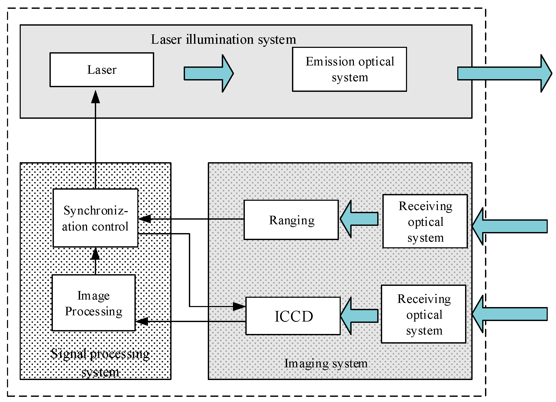
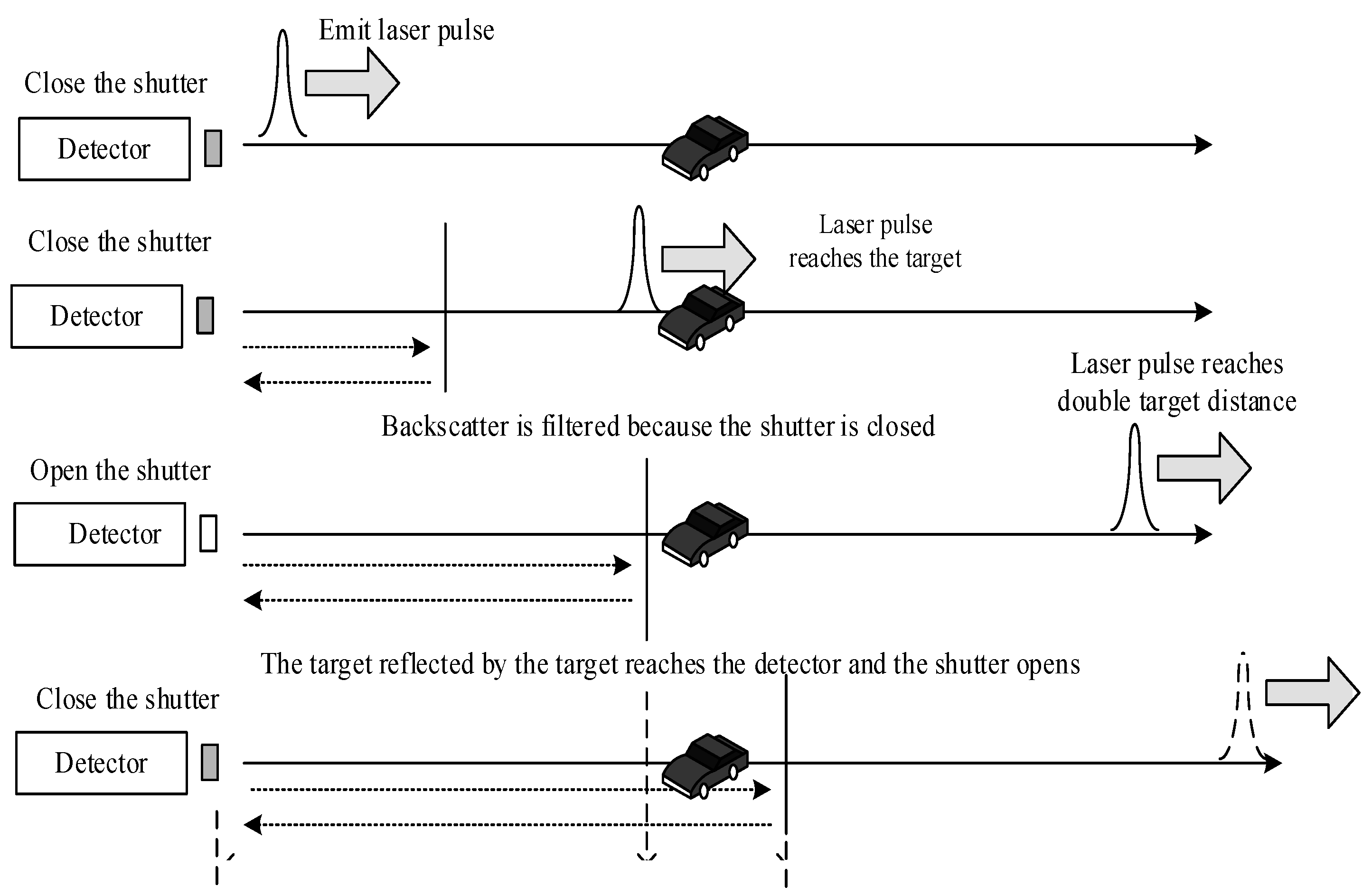
2. Range-Gated Imaging System

A typical gated imaging system is shown in Figure 1. It mainly includes the following sub-systems: (1) Laser illumination system, the laser illuminates the target through the emission optical system; (2) Imaging system, the ICCD detector receives the reflectance light from the target through the receiving optical system, and the target is gated and imaged by the ranging information; (3) Signal processing system, which is responsible for synchronous control and image processing of the laser and ICCD [6].

The principle of gated imaging is shown in Figure 2 [7,8]. The laser emits a pulse at time T. At this time, the detector shutter is closed. After a period of time $t_0$, the target reflectance light reaches the detector. At this time, the detector shutter is opened by the high-precision synchronization control module, the target at a distance of $R_1=c{t}_0/2$ can be imaged, where $c$ is the speed of light in a vacuum. After receiving the pulsed light, the shutter closes again and waits for the next pulse to come, and then cycle the imaging. It can be seen from the imaging principle that gated imaging only images the interested area and can artificially shield out irrelevant information. It is not only widely used in the detection of hidden target detection and underwater target detection, but also has important applications in rain, snow and foggy weather imaging.

3. Adaptive Homomorphic Filtering

3.1. Homomorphic Filtering Algorithm

A homomorphic filtering algorithm has two major functions. On the one hand, it can increase the contrast of the image, on the other hand, it can compress the image appropriately in the dynamic range. An image can be represented by the two-dimensional function $f(x,y)$. $(x,y)$ represents the coordinates of the pixel point, and $f(x,y)$ is the value of that point. $f(x,y)$ can be expressed by the incident light component $i(x,y)$ and the reflectance light component $r(x,y)$ [9,10]:

$$f(x,y)=i(x,y)\cdot r(x,y)$$

(1)

Take logarithms for both sides of Equation (1):

$$\ln f(x,y)=\ln i(x,y)+\ln r(x,y)$$

(2)

Equation (2) indicates that the sum of the logarithms of the incident light component and the logarithm of the reflectance light component is equal to the logarithmic value of the image brightness value. A Fourier transform is applied to Equation (2) to transform the function space and frequency domains:

$$F\{\ln f(x,y)\}=F\{\ln i(x,y)\}+F\{\ln r(x,y)\}$$

(3)

Equation (3) can be briefly written as:

$$F(u,v)=I(u,v)+R(u,v)$$

(4)

where $I(u,v)$ is defined as illuminance function and its spectrum is mostly in the low frequency range. $R(u,v)$ is defined as reflection function and its spectrum is mostly in the high frequency range.

Homomorphic filter function $H(u,v)$ determines the enhancement effect of the image, the function designed in this paper is based on the need to increase the reflectance component $r(x,y)$ and reduce the incident component $i(x,y)$, different gain coefficients are used for low frequency and high frequency components. Hence the characteristics of $H(u,v)$ are as follows: for low-frequency areas in the image, $H(u,v)<1$; for low-frequency areas in the image, $H(u,v)>1$. The mathematical expression is:

$$H(u,v)\cdot F(u,v)=H(u,v)\cdot I(u,v)+H(u,v)\cdot R(u,v)$$

(5)

Inverse transformation of Equation (5) to the space domain gives:

$$h_f(x,y)=F^{-1}[H(u,v)\cdot I(u,v)]+F^{-1}[H(u,v)\cdot R(u,v)]$$

(6)

If $h_i(x,y)=F^{-1}[H(u,v)\cdot I(u,v)]$, $h_r(x,y)=F^{-1}[H(u,v)\cdot R(u,v)]$, Equation (6) can be expressed as:

$$h_f(x,y)=h_i(x,y)+h_r(x,y)$$

(7)

Taking the exponent on both sides of Equation (7):

$$g(x,y)=\exp \left|h_f(x,y)\right|=\exp \left|h_i(x,y)\right|\cdot \exp \left|h_r(x,y)\right|$$

(8)

When the Fourier inverse transforms back to the spatial domain, there are both real and imaginary parts, but the pixels of the image are represented by real numbers, so only the real part of the result is taken, where $\left|\right|$ represents the real part of an extraction function.

If $i_o(x,y)=\exp \left|h_i(x,y)\right|$, $r_o(x,y)=\exp \left|h_r(x,y)\right|$, Equation (8) can be expressed as:

$$g(x,y)=i_o(x,y)\cdot r_o(x,y)$$

(9)

where $g(x,y)$ is a two-dimensional function processed from the original image $f(x,y)$, representing the enhanced image. $i_o(x,y)$ represents the illuminance function after the inverse operation, $r_o(x,y)$ represents the reflection function after the inverse operation.

The steps for enhancing using the homomorphic filtering algorithm [11] are shown in Figure 3.

In this paper, an improved second-order Butterworth filter is used, and it can be expressed as follows [12]:

$$H(u,v)=r_1-r_2[\frac{1}{1+c\cdot {({\rho }_c/\rho )}^4}]$$

(10)

where $\rho ={[{(u-u_0)}^2+{(v-v_0)}^2]}^{1/2}$ and it is the distance from frequency $(u,v)$ to the center of the filter $(u_0,v_0)$. When $(u_0,v_0)=(0,0)$, $\rho ={[u^2+v^2]}^{1/2}$. ${\rho }_c$ is the cut-off frequency. The selection of cut-off frequency is usually difficult, which is mainly based on empirical judgment, and its value can be obtained by calculating the median value of $\rho$. $c$ is a value that controls the shape of the filter, that is, the steepness (slope) from low frequency to high frequency. The larger the value, the steeper the slope band. When $\rho /{\rho }_c>>1$, $r_H=r_1$. When $\rho /{\rho }_c<<1$, $r_L=r_1-r_2$.

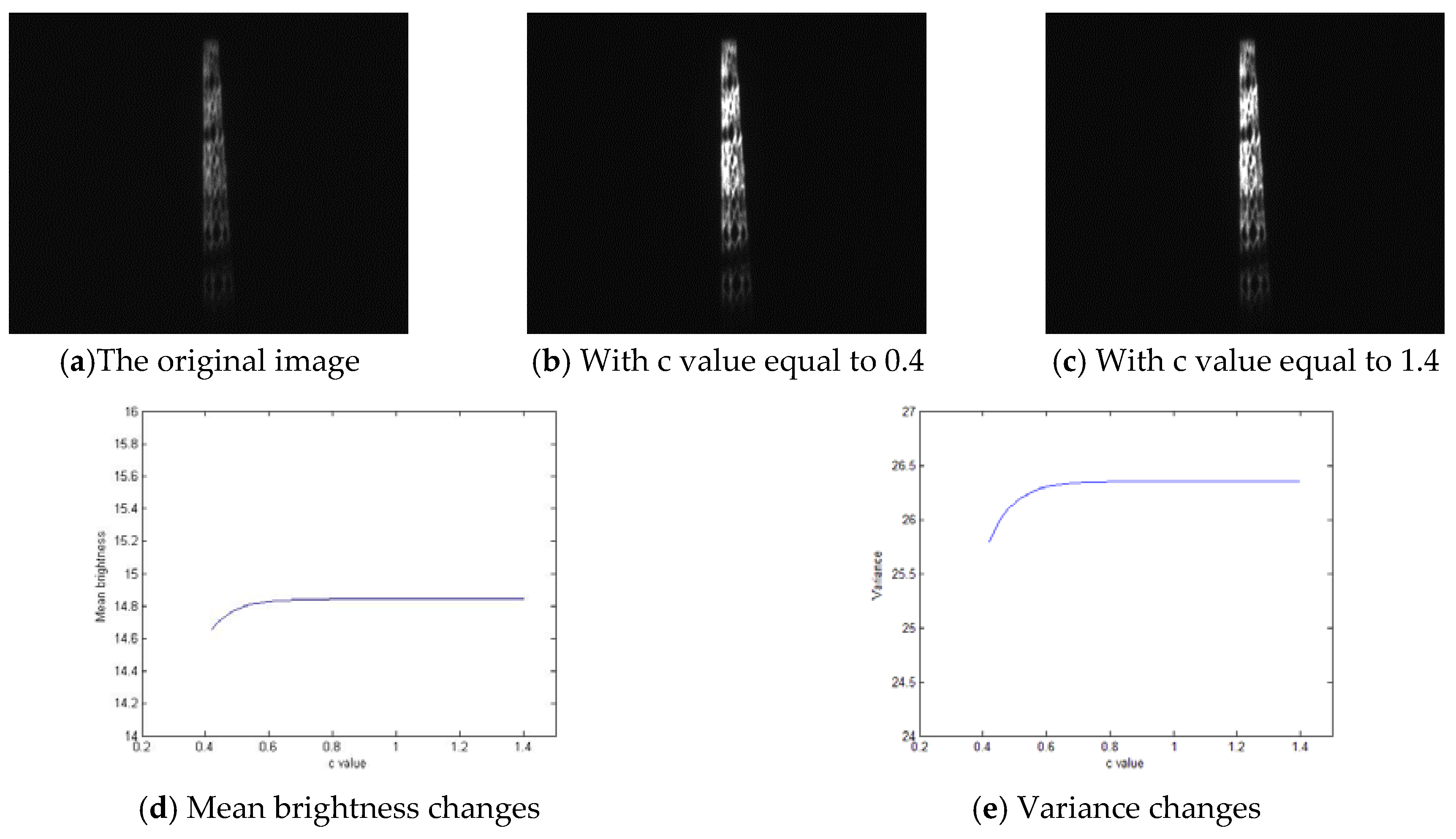
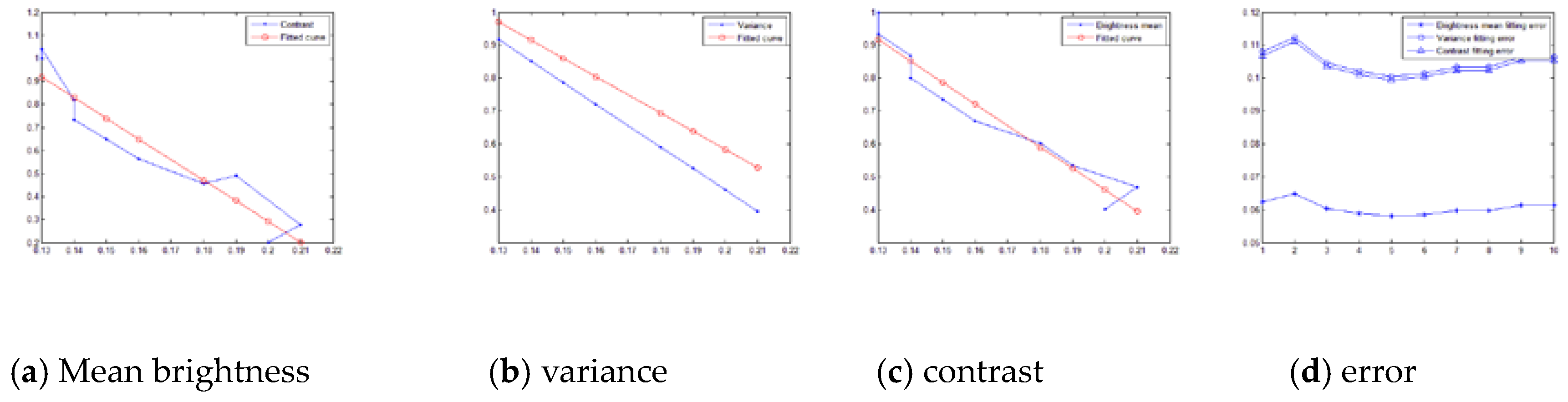
3.2. Adaptive Homomorphic Filtering Algorithm

When the laser gating imaging system has different imaging conditions, the brightness and contrast of the image are also different. The target shown in Figure 4 is a cluster of balloons. Figure 5a,b shows the gating imaging of the target using the distance gating system under imaging conditions at different time of day. Figure 5a is the image obtained at night, and Figure 5b is the image obtained during the day. When imaging at night, the laser illuminates the target, and other unilluminated parts entering the ICCD can be ignored. During daytime imaging, due to the influence of sunlight, the stray light entering the ICCD greatly increases, and the brightness of the entire image will also greatly increase. It can be seen from the Figure 5a that the imaging background in Figure 5a is relatively single, and the target is more prominent in the entire image. The algorithm in Section 3.1 is used to enhance the image and the results are shown in Figure 5c. It can be seen from the Figure 5c that the contrast between the target and the background is increased, and the details of the target are also enhanced. Figure 5b is enhanced with the same parameters, and the result is shown in Figure 5d. As can be seen from Figure 5d, the effect of enhancement processing is not good. Although the image brightness increased, the image details of the target were overwhelmed. The enhancement effect is mainly related to $c$ in homomorphic filtering. How to choose the appropriate $c$ to enhancement image according to the characteristics of the image is the main content of this section.

From Figure 5, we can know that the biggest difference between the images is brightness and contrast, but brightness and contrast cannot essentially classify images. In image enhancement, the overall distribution of image pixels is generally described with a histogram distribution [13]. A histogram is a table that represents the number of pixels with a certain value in an image. Therefore, the histogram has 256 abscissa values to represent the pixel values, and the vertical axis represent the distribution. The histogram of the statistical image is shown in Figure 6. Figure 6a is the histogram of Figure 5a. Figure 6b is the histogram of Figure 5b.

Compared to Figure 6, the brightness of the image in imaging condition 1 is more concentrated than that in imaging condition 2. The pixel distribution of the image under imaging condition 2 is similar to a Gaussian distribution. There are few pixels with brightness of 0 and 255, and there is a natural transition between pixels. The image brightness distribution under imaging condition 1 is generally close to 0, it is closer to the exponential distribution, and the pixels have strong discrimination. As can be seen from the above analysis, the histograms vary greatly between different imaging conditions. From the perspective of the histogram, the target is divided into two categories, one is a histogram-like Gaussian distribution, called class I, and other is the one whose image brightness is close to an exponential distribution, called class II. The histogram can be regarded as a quadratic function fitting, class I image is a complete quadratic function with a negative quadratic term, and class II image is the left part of the quadratic function with a positive quadratic term. Whether the image is class I or II can be determined by the positive and negative quadratic terms of the fitted quadratic function. Figure 7a shows the histogram and fitting curve of imaging 1, and Figure 7b shows the histogram and fitting curve of imaging 2. The fitting parameters are shown in

Table 1. Quadratic function fitting parameters.

Imaging Conditions	Quadratic Term Coefficient	First-Order Coefficient	Constant
Condition 1	0.6996	−216.4452	14,131.8952
Condition 2	−0.2139	51.1179	−791.8378

.

In order to find the relationship between imaging and homomorphic filter parameter c, different c values are used for processing. Let’s discuss night images first. Figure 8a is an image at night, while Figure 8b,c corresponds to the processing results of parameters c of 0.4 and 1.4, respectively. The homomorphic filtering parameter c increases from 0.4, with a step of 0.02 and a cycle step of 50 times, that is, the value of c changes from 0.4 to 1.4. The mean brightness and variance of the image processed after 50 cycles are shown in Figure 8d,e.

It can be seen that in the night image, the processed image changes little when the c value changes (greater than a certain value, such as 0.4), and the floating range of its mean value and variance does not exceed 1, and it can be considered that there is no change, so it is concluded that in the night image, the c value selection (greater than a certain value, such as 0.4) has little relationship with the image enhancement effect, so, for the class I image, the value of c is fixed at 0.5.

The same method is used to analyze the relationship between daytime imaging and c parameter. Parameter c increases from 0.1, with a step of 0.01 and a step of 100 cycles. The change of c value is 0.1–1.1. The above processing is carried out on the 10 images respectively, and the mean brightness value and target variance floating range of the processed images are calculated, the result is shown in Figure 9.

It can be seen from Figure 9 that in different imaging, when the value of c changes, the brightness and variance of the image change greatly. Therefore, when processing images taken during the day, a suitable c value must be selected according to different brightness, rather than the fixed value just like the night image. Based on this judgment, 10 images are still selected, and the best corresponding c value of the enhancement effect is found by the way of human eye judgment, and the mean brightness value, variance value and contrast of the original image are calculated as shown in

Table 2. Mean brightness, variance, contrast and optimal c value of the original image.

Imaging	1	2	3	4	5	6	7	8	9	10
Optimal c	0.2	0.21	0.19	0.18	0.16	0.15	0.14	0.14	0.13	0.13
Mean	66.07	77.13	88.09	99.15	110.11	121.09	131.93	142.85	153.64	164.70
Variance	12.45	19.53	16.60	18.69	20.75	22.28	28.69	25.05	26.37	27.67
Contrast	155.1	211.40	375.79	349.36	430.83	496.59	561.67	627.56	795.782	765.73

. With the best c value as the x-axis, the curves fitting with the mean brightness value, variance value and contrast value are shown in Figure 10. The mean brightness, variance and contrast are defined as:

$$mean=\frac{1}{MN}{\displaystyle \sum _{x=1}^M{\displaystyle \sum _{y=1}^{N}f(x,y)}},variance=\frac{1}{MN}{\displaystyle \sum _{x=1}^M{\displaystyle \sum _{y=1}^N(f(x,y)-mean)}},contrast=\frac{\left|{\mu }_T-{\mu }_B\right|}{{\mu }_T+{\mu }_B}$$

(11)

where M is the number of rows in the image, N is the number of columns. The processed image is represented by $f(x,y)$. ${\mu }_T$ is the mean brightness of the target, ${\mu }_B$ is the mean brightness of the background.

It can be seen from the Figure 10d that the closest fitting curve to the data is the mean brightness fitting curve, so y = −1073.1783x + 290.4094 (fitted curve of mean brightness) is selected as the equation to predict the best c value. So, when processing class II image, the following empirical formula is obtained as follows:

$$c=-(m-290)/1073$$

(12)

where $m$ is mean gray value of the entire image.

4. Total Variation Noise Reduction Model

Rudin proposed a noise reduction algorithm based on total variation theory, the core idea of the algorithm is that if there is no noise in the image, its total variation will be smaller, if there is noise, its total variation will be larger. Therefore, minimizing the total variation of the image can reduce the noise in the image. This method is called total variation noise reduction model (TV model) [14,15].

Assuming $f(x,y)$ is the original image and the original image contains no noise, add noise $n(x,y)$ to $f(x,y)$ with variance at ${\sigma }^2$ and zero mean. The image after adding noise can be expressed as:

$$f_o(x,y)=f(x,y)+n(x,y),(x,y)\in \mathsf{\Omega }$$

(13)

The problem of reducing image noise is transformed into the problem of obtaining the minimum total variation, which can be expressed as [16]:

$$\min TV(f)={\displaystyle {\int }_{\mathsf{\Omega }}^{}\sqrt{{\left|\nabla f\right|}^2}dxdy=}{\displaystyle {\int }_{\mathsf{\Omega }}^{}\sqrt{f_x{}^2+f_y{}^2}dxdy}$$

(14)

where $\nabla$ represents the gradient operator.

Constrained conditions can be obtained from noise characteristics:

$${\displaystyle {\int }_{\mathsf{\Omega }}^{}fdxdy=}{\displaystyle {\int }_{\mathsf{\Omega }}^{}{f}_{0}dxdy}$$

(15)

$$\frac{1}{\left|\mathsf{\Omega }\right|}{\displaystyle {\int }_{\mathsf{\Omega }}^{}{(f-f_0)}^{2}dxdy=}{\sigma }^2$$

(16)

where $\sigma$ is variance of noise, $\mathsf{\Omega }$ is the area where the image is located, and the image area is expressed as $\left|\mathsf{\Omega }\right|$. Then the total variation energy functional expression of the image is:

$$J[f]={\displaystyle {\int }_{\mathsf{\Omega }}^{}\sqrt{{\left|\nabla f\right|}^2}dxdy+\frac{\lambda }{2}{\displaystyle {\int }_{\mathsf{\Omega }}^{}{(f-f_0)}^{2}dxdy}}$$

(17)

where $\lambda$ is Lagrange factor.

Taking the derivative of $f$ for $J[f]$, we can get Euler-Lagrange equation:

$$\frac{\partial J}{\partial f}=-\nabla \cdot (\frac{\nabla f}{\left|\nabla f\right|})+\lambda (f-f_0)$$

(18)

When $\frac{\partial J}{\partial f}=0$, discrete numerical calculations of the Equation (18), the Gauss-Jacobi iterative algorithm is used to obtain the final noise reduction image.

It can be seen from Equation (18) that in the smooth part of the image (the non-edge region), the value of $\nabla f$ is relatively small, and the corresponding value of $1/\nabla f$ (also called the diffusion coefficient) will be relatively large. Large diffusion coefficient, the diffusivity in the smooth part of the image will be stronger, and the noise reduction effect will be more obvious. However, at the edge of the image, the value of $\nabla f$ will increase due to the abrupt change in the gray value, resulting in a decrease in the diffusion coefficient, thereby retaining the edge portion of the image. Therefore, total variation noise reduction model not only has excellent noise reduction effects, but also retains edge features to the maximum extent.

5. Experimental Results and Analysis

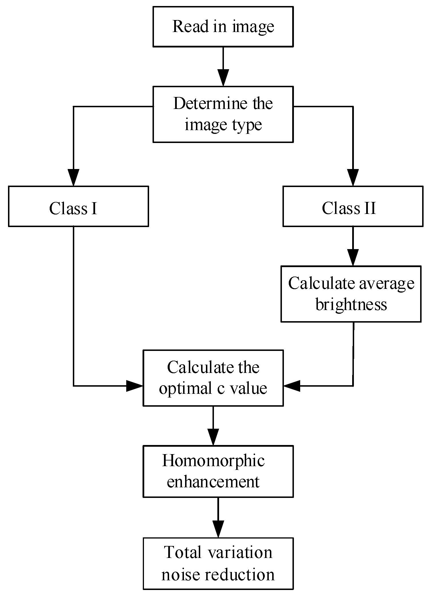
5.1. Algorithm Flow

According to the description in Section 3 and Section 4, the flowchart of the adaptive algorithm is shown in Figure 11. Firstly, the type of image is determined. Whether the image is class I or II can be determined by the positive and negative quadratic terms of the fitted quadratic function. Then the optimal value of $c$ is determined for homomorphic filtering. In the homomorphic filter algorithm, the value of cut-off frequency ${\rho }_c$ is usually given a fixed value. In the formula of $H(u,v)$, we multiply ${({\rho }_c/\rho )}^4$ and c into $c\cdot {({\rho }_c/\rho )}^4$. The value of $H(u,v)$ can also be changed by adjusting the value of c, thereby changing the filtering performance of the filter. Therefore, the adjustment of c indirectly changes the cut-off frequency. Finally, total variation noise reduction is performed.

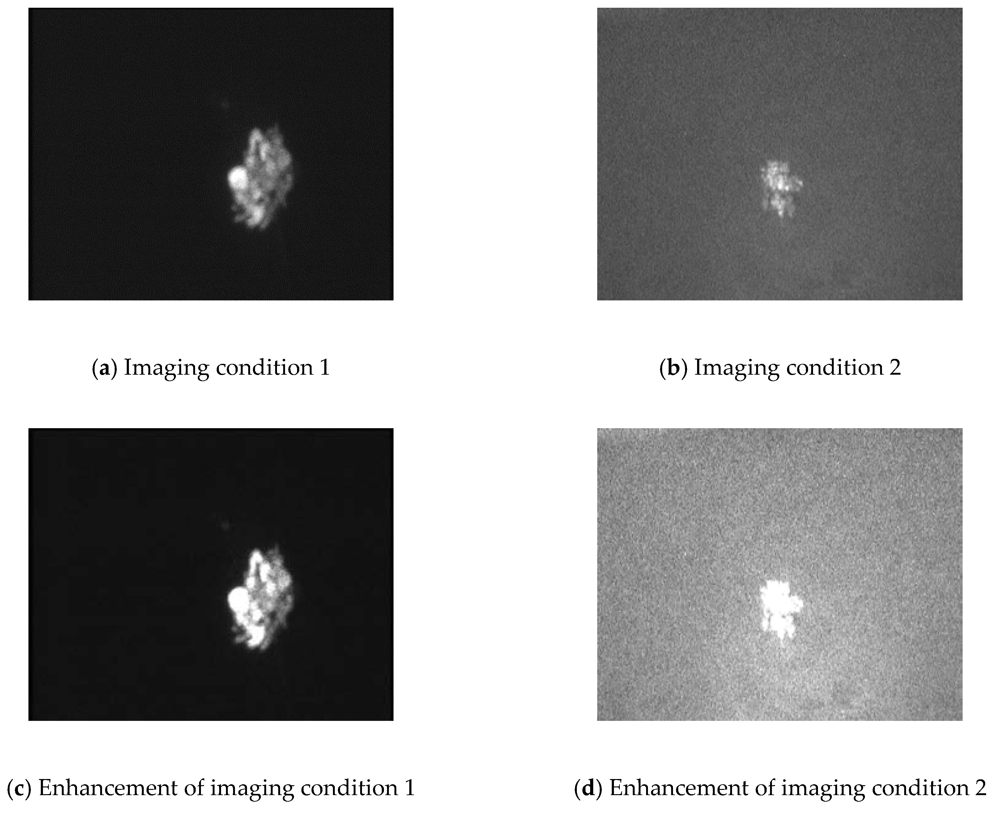
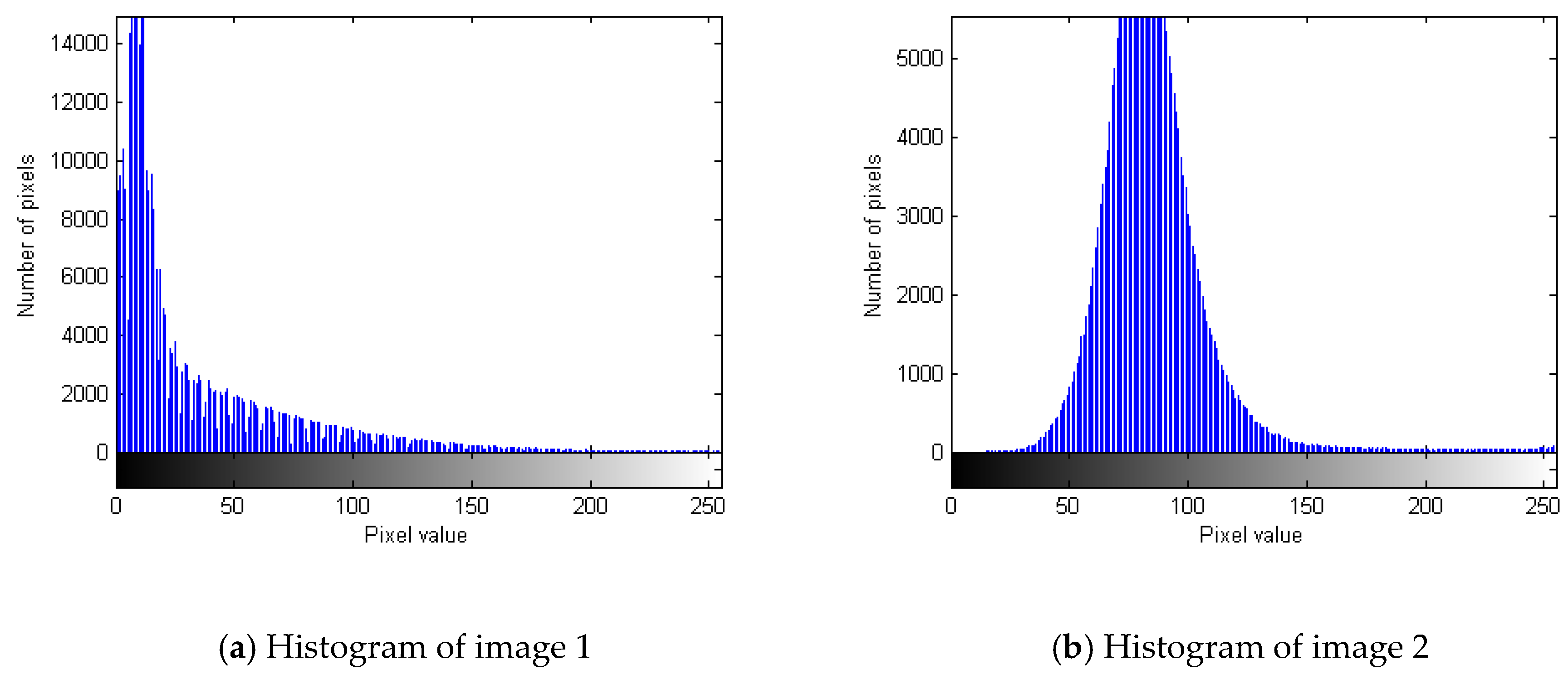
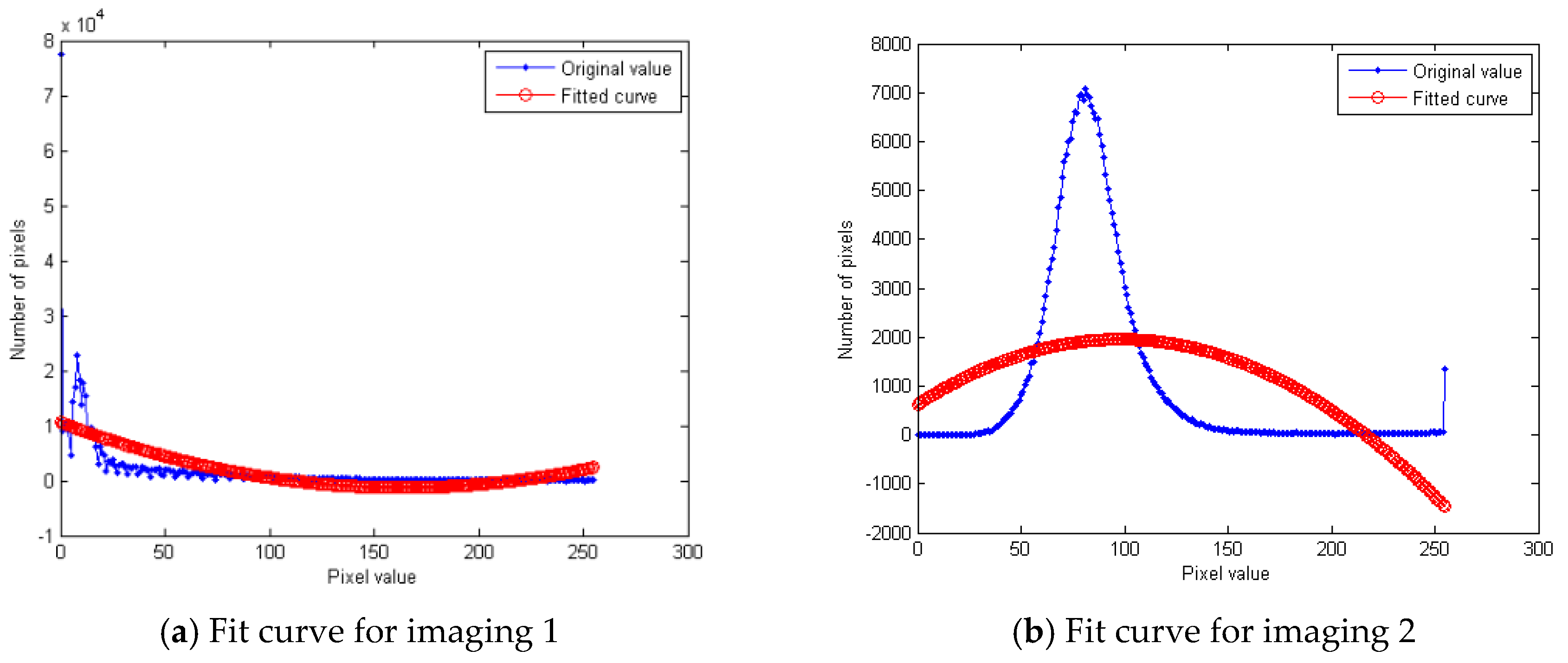
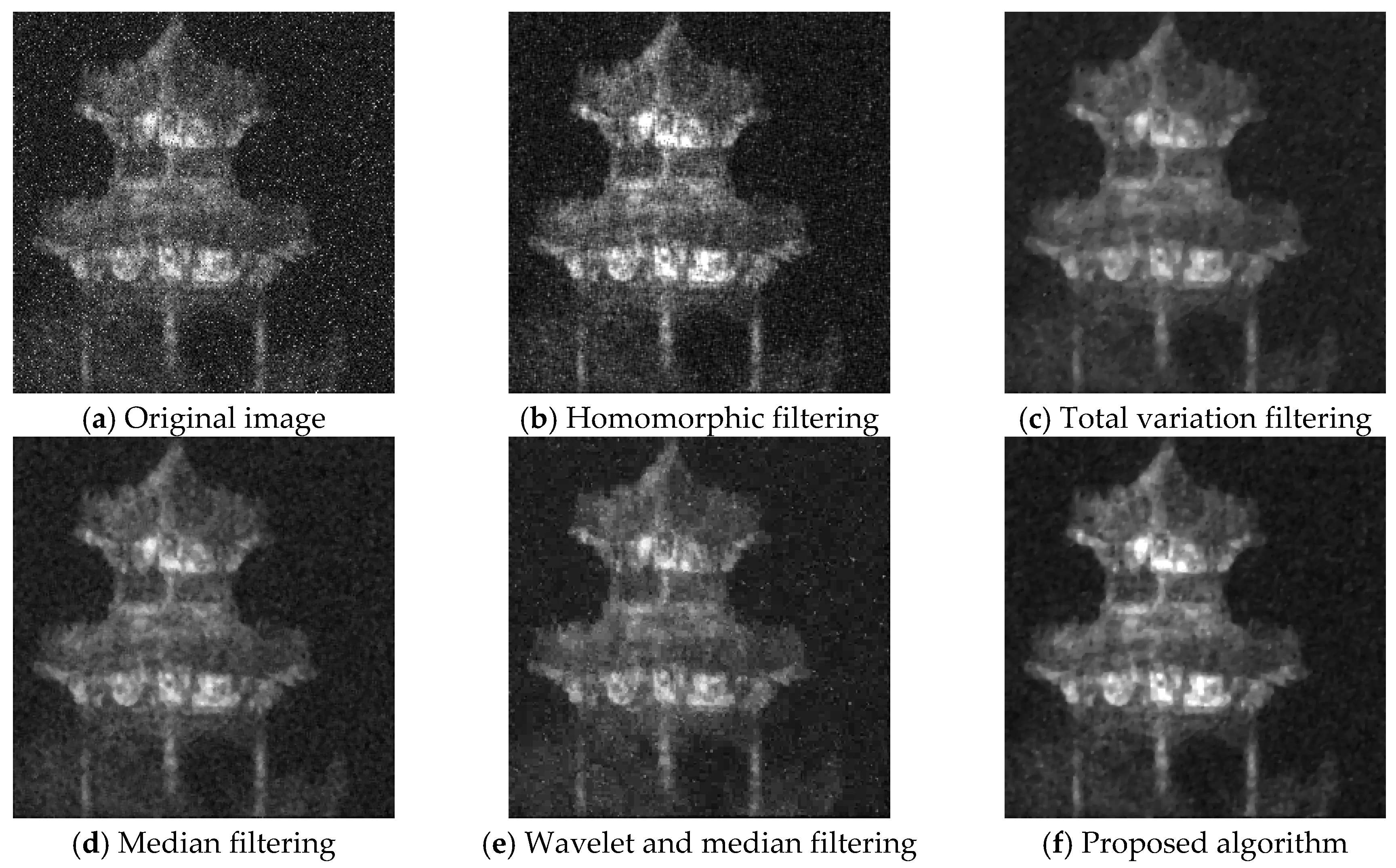
5.2. Processing of Class I Images

In order to verify the effectiveness of the algorithm in this paper, a class I image is processed. The gated image formed by the pavilion is shown in Figure 9a. The quadratic term of the fitted curve is 0.0166, and $c=0.5$. Some filtering algorithms are selected for image processing, such as median filter noise reduction, wavelet and median filter noise reduction and other algorithms, and compared with the noise reduction results obtained by the proposed algorithm. The filter parameters were selected as $r_H=1.5,r_L=0.1,c=0.5$, and the brightness, signal-to-noise ratio, average gradient and edge intensity were used to analyze the processed results.

The algorithms are implemented using MATLAB 8.3.0.532(MATLABR2014a, Mathworks, USA), and the filtered results are shown in Figure 12. Figure 12a is laser image of a pavilion formed by range-gated imaging system at night, and the image size is 256 × 256. The target image histogram and fitting curve are shown in Figure 13. Figure 12a is the original image with superimposed impulse noise; Figure 12b is the homomorphic filtering noise reduction image; Figure 12c is the total variation filtering noise reduction image and Figure 12d is the median filtering noise reduction image. This method is to set the value of each pixel to the median of all pixels in a neighborhood window. The filtering window in the paper is 3 × 3 pixels. Figure 12e is wavelet and median filtering noise reduction image. The image is dealt with median filter firstly. Then the image is decomposed with the wavelet. The low frequency parts of decomposed images are processed by the threshold. Finally, the image is reconstructed by the processed wavelet coefficients. Figure 12f is the proposed algorithm noise reduction image.

The edge strength is defined as:

$$Edgestrength=\frac{1}{MN}{\displaystyle \sum _{x=1}^M{\displaystyle \sum _{y=1}^N\sqrt{g_x{(x,y)}^2+g_y{(x,y)}^2}}}$$

(19)

where M is the number of rows in the image, N is the number of columns. The processed image is represented by $g(x,y)$ $g_x(x,y)$ and $g_y(x,y)$ represent the gradient in x and y directions.

As can be seen from Figure 12, the algorithm proposed in this paper has an obvious enhancement effect while reducing noise. As can be seen from Figure 13, quadratic function fitting basically describes the histogram trend of images. It can be seen from

Table 3. Comparison of performance indicators of different algorithms.

Parameters.	Original Image	Homomorphic Filtering	Total Variation Filtering	Median Filtering	Wavelet and Median Filtering	Proposed Algorithm
Brightness	38.8453	58.4783	35.2163	34.5822	35.1859	53.0877
Signal to Noise Ratio	12.6069	11.2899	23.2361	19.1329	17.6084	21.2822
Average Gradient	6.0313	20.5307	3.7252	6.1149	9.6674	19.2859
Edge Strength	58.1744	141.1252	37.4476	61.7853	85.3768	151.0584
Time(s)		0.2321	1.3564	0.1268	1.4238	1.4092

that while the proposed algorithm improves the contrast and makes the target more prominent, the SNR also improves. The results in Table 3 are also basically consistent with the visual effect of Figure 12. The algorithm time is between homomorphic filtering and total variation filtering, smaller than wavelet and median filtering.

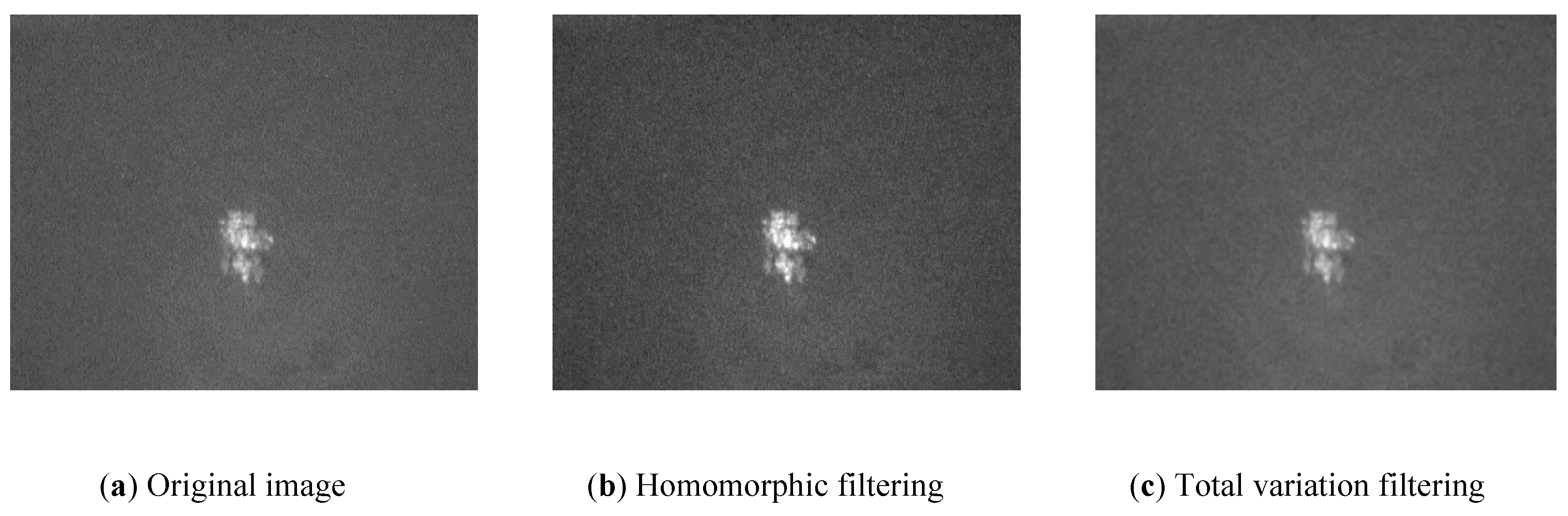
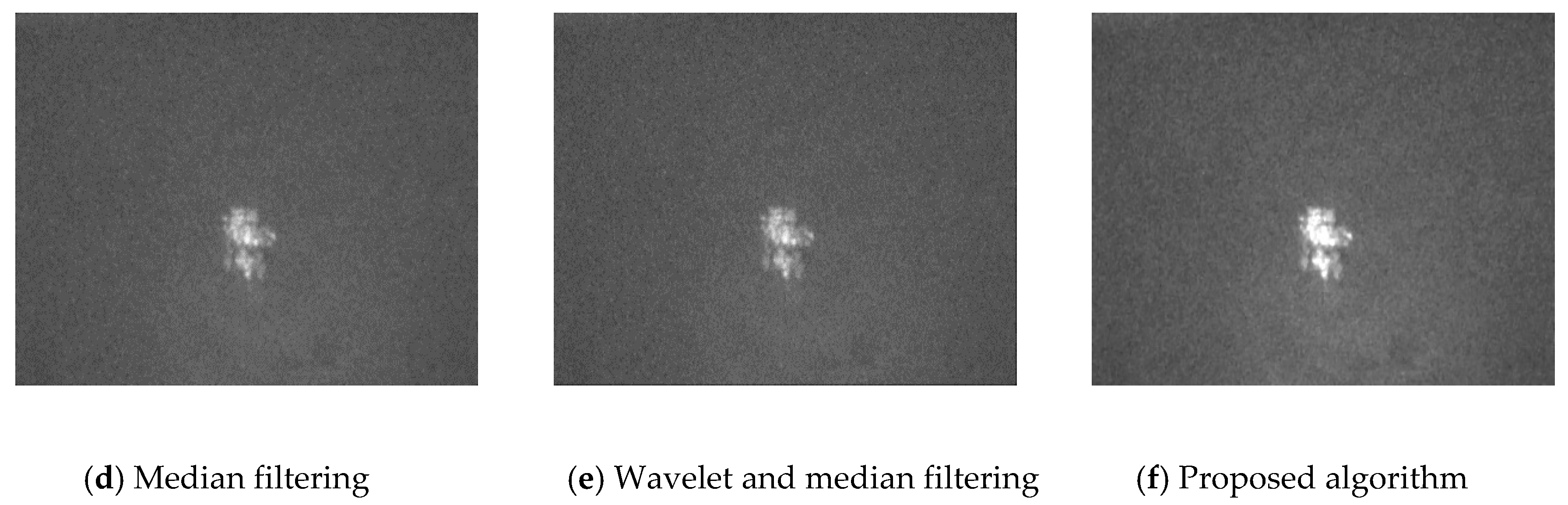
5.3. Processing of Type II Images

For the type II image, the quadratic term of the fitting curve is −0.1731, as shown in Figure 14. Figure 14a shows the gated image formed by the balloon. The average brightness value is 89.2235 (the average brightness value is the average value of the entire image, and it is the average brightness value of the target area in the filtered indicator). According to the relationship between the optimal c value and the variance, $c=-(m-290)/1073$, the optimal value of $c$ can be determined as 0.1871. Figure 15a is a laser image of a cluster of balloons formed by range-gated imaging system during the day, and the image size is 256 × 256. The proposed algorithm is compared with other noise reduction algorithms, and the results are shown in Figure 15b–d. Filtered indicators are shown in

Table 4. Comparison of performance indicators of different algorithms.

Parameters	Original Image	Homomorphic Filtering	Total Variation Filtering	Median Filtering	Wavelet and Median Filtering	Proposed Algorithm
Brightness	108.5561	123.1349	112.7245	112.9057	112.9012	129.1970
Signal to Noise Ratio	9.4461	11.2899	10.5266	12.4359	11.2216	14.6058
Average Gradient	4.0522	6.2278	3.7317	4.2416	5.4886	7.6992
Edge Strength	49.0059	58.1435	45.0113	40.9643	43.0269	63.0800
Time(s)		0.3528	1.4271	0.1021	1.6291	1.5015

.

As can be seen from the Figure 15, various algorithms have certain noise reduction effects, and homomorphic filtering has a significant enhancement effect; total variation filtering removes background interference noise well; median filtering has some ambiguity; the combination of wavelet and median algorithm still has strong impulse noise after noise reduction, but the edge details are well preserved. The proposed algorithm in this paper has obvious enhancement effect while reducing noise. A comparison of performance indicators is shown in Table 4. From the perspective of brightness, average gradient and edge strength, the proposed algorithm works better than the total variation filtering, median filtering and wavelet combined median algorithm. The proposed algorithm significantly improves the contrast, makes the target more prominent, and achieves the expected effect. It can better adjust the image brightness and facilitate subsequent processing.

6. Conclusions

According to the analysis of the characteristics of the laser image, it can be known that the image quality of the laser active imaging system is affected by various factors, which will cause the signal to noise ratio of the image to decrease, and further denoising processing is required. Especially for moving target imaging, image denoising enhancement can only be processed in a single frame. Based on the characteristics of the laser image, an improved algorithm based on homomorphically filtered and total variation is proposed. An adaptive enhancement algorithm is used for images taken in different time periods. The effectiveness of the algorithm is verified by using experimentally acquired images. The proposed algorithm can reduce the noise while preserving the edge details. From the perspective of brightness, average gradient and edge strength, the proposed algorithm works better than traditional single algorithm.

7. Future Work Prospects

In the next step of the work, there are two important things to do. The first is to improve the quality of laser image by using a deep learning method. The second is to install an adaptive system on the imaging system. Deep learning denoising methods on a large set of test images is the future trend, but laser images based on range-gated do not have an image library. The current images are neither representative nor systematic, and the number is very small. In the next step, we will establish our own laser image database and use a deep learning method to reduce the noise.

Besides, the adaptive optics (AO) system is also an effective way to improve the quality of laser active imaging. Generally, before the laser beam reaches the target, the phase distortion introduced by the optical element deformation, non-uniform medium, turbulent atmosphere and other disturbance factors in the transmission path, including the laser light source itself due to mirror imbalance, medium thermal effect, mechanical vibration and other factors will lead to the beam quality degradation. AO can compensate this distortion in real time, which is helpful to improve the uniformity of the laser output beam energy distribution, thereby improving the utilization rate of laser energy, improving the image quality and reduce the requirement of laser output laser energy power. A typical adaptive optical system consists of three parts: the wavefront corrector, the wavefront sensor and the wavefront controller, as shown in Figure 16.

In the figure, the wavefront sensor is used to detect the static and dynamic wavefront errors in the optical system in real time. The wavefront controller is used to process the wavefront distortion signal from the wavefront sensor in real time and calculate the wavefront error, thereby obtaining the voltage control signal needed on the wavefront corrector. The wavefront corrector, which consists of deformable mirrors and fast tilt mirrors, is the executive component of the adaptive optical system. It produces a wavefront which is conjugate with the input distorted wavefront, and the calibrated beams approach to the plane waves, finally improving the resolution of the imaging system or the beam quality of the laser transmission system.

In addition, the Gaussian beam can be shaped into a laser beam with uniform distribution by AO system. Generally, the output beam of laser is approximately Gaussian distribution in spatial morphology, which is called Gaussian beam, as shown in Figure 17a. For laser imaging, we hope that the output light of laser is uniform, so that the light irradiated to the target is also uniform, which is conducive to improving the imaging quality, As shown in Figure 17b. The AO system modulates the complex amplitude distribution of the incident light field by controlling the deformed mirror and compensates the aberration of the system by changing the surface shape to achieve beam shaping. It has the characteristics of flexible control, good adaptability, high efficiency of light energy transmission and high damage threshold.

References

1. Chen CL, P.; Liu, L.; Chen, L.; Tang, Y.Y.; Zhou, Y. Weighted Couple Sparse Representation with Classified Regularization for Impulse Noise Removal. IEEE Trans. Image Process. 2015, 24, 4014–4026. [Google Scholar] [CrossRef] [PubMed]
2. Minru, B.; Shihuan, G. TV-MCP:A New Method for Image Restoration in the Presence of Impulse Noise. Ournal Hunan Univ. (Nat. Sci.) 2018, 45, 126–130. [Google Scholar]
3. Yin, L.; Chen, B.H.; Li, Y. Highly accurate image reconstruction for multimodal noise suppression using semisupervised learning on big data. IEEE Trans. Multimed. 2018, 20, 3045–3056. [Google Scholar] [CrossRef]
4. Ian, Z.; Tong, Z.; Ma, Y.; Wang, M.; Ia, S.; Chen, X. Laser beam modulation with a fast focus tunable lens for speckle reduction in laser projection displays. Opt. Lasers Eng. 2020, 126. [Google Scholar]
5. Norashikin, Y.; Nidal, S.; Aamir, S.M. Subspace-based technique for speckle noise reduction in SAR images. Ieee Trans. Geosci. Remote Sens. 2014, 52, 6257–6271. [Google Scholar]
6. Ian, B.; Stuart, D.; Eremy, C. A Low Noise, Laser-Gated Imaging System for Long Range Target Identification. Proc. SPIE 2004, 5406, 133–144. [Google Scholar]
7. Guo, H.; Sun, H.; Wang, S.; Fan, Y.; Li, Y. Study on super-resolution three-dimensional range-gated imaging technology. In Proceedings of the 9th International Conference on Graphic and Image Processing, Qingdao, China, 14–16 October 2017; Volume 10615. [Google Scholar]
8. Hu, P. Weak Signal Detection Research on Gain Modulated Imaging Ladar; Harbin Institute of Technology: Harbin, China, 2013; pp. 14–24. [Google Scholar]
9. Kaur, K.; Jindal, N.; Singh, K. Improved homomorphic filtering using fractional derivatives for enhancement of low contrast and non-uniformly illuminated images. Multimed. Tools Appl. 2019, 78, 27891–27914. [Google Scholar] [CrossRef]
10. Zhang, C.; Liu, C.; Xing, W. Color image enhancement based on local spatial homomorphic filtering and gradient domain variance guided image filtering. J. Electron. Imaging 2018, 27, 063026. [Google Scholar] [CrossRef]
11. Tseng, C.; Lee, S. A Weak-Illumation Image Enhancement Method using Homomorphic Filter and Image Fusion. In Proceedings of the IEEE Global Conference on Consumer Electronics, Kyoto, Japan, 11–14 October 2016. [Google Scholar]
12. Liu, Z.; Zou, J.W.; Zhang, J.; Yang, H. The Homomorphic Enhancement of Infrared Image in Fuzzy Field. Laser Infrared 2007, 37, 87–89. [Google Scholar]
13. Fan, Y.; Zhao, H.; Sun, Y. Adaptive enhancement algorithm of laser image based on histogram fitting and brightness decision. Laser Infrared 2015, 8, 21. [Google Scholar]
14. Kumar, M.; Diwakar, M. A new exponentially directional weighted function based CT image denoising using total variation. J. King Saud Univ. Comput. Inf. Sci. 2019, 31, 113–124. [Google Scholar]
15. Kumar, A.; Ahmad, M.; Swamy, M. Tchebichef and Adaptive Steerable-Based Total Variation Model for Image Denoising. IEEE Trans. Image Process. 2019, 28, 2921–2935. [Google Scholar] [CrossRef] [PubMed]
16. Bredies, K.; Vicente, D. A perfect reconstruction property for PDE-constrained total-variation minimization with application in Quantitative Susceptibility Mapping. Esaim-Control Optim. Calc. Var. 2019, 25, 83. [Google Scholar] [CrossRef]
Figure 1. Schematic diagram of a typical gated imaging system.
Photonics 07 00030 g001
Figure 2. Gated imaging schematic.
Photonics 07 00030 g002
Figure 3. Homomorphic filtering flowchart.
Photonics 07 00030 g003
Figure 4. Target image.
Photonics 07 00030 g004
Figure 5. (ad) Enhancement effect under different imaging conditions.
Photonics 07 00030 g005
Figure 6. (a,b) The histograms of the statistical image.
Photonics 07 00030 g006
Figure 7. (a,b) Histogram and quadratic function fitting curve.
Photonics 07 00030 g007
Figure 8. (ae) Mean brightness and variance changes corresponding to different parameters in nighttime imaging.
Photonics 07 00030 g008
Figure 9. (a,b) The mean brightness and variance changes corresponding to different parameters during daytime imaging.
Photonics 07 00030 g009
Figure 10. (ad) Mean brightness, variance, contrast and fitting curve.
Photonics 07 00030 g010
Figure 11. Flowchart of the adaptive algorithm.
Photonics 07 00030 g011
Figure 12. (af) Noise reduction effect of different algorithms.
Photonics 07 00030 g012
Figure 13. (a,b) Histogram and fitting curve of the target image.
Photonics 07 00030 g013
Figure 14. (a,b) Histogram and fitting curve of the target image.
Photonics 07 00030 g014
Figure 15. (af) Reduction effect of different algorithms.
Photonics 07 00030 g015aPhotonics 07 00030 g015b
Figure 16. Composition of an AO system.
Photonics 07 00030 g016
Figure 17. (a,b) Shaping of a Gaussian beam.
Photonics 07 00030 g017