1. Introduction
For many years, photonic crystals (PCs) of metal-dielectric structures designed to control and manipulate the propagation of electromagnetic fields have been widely studied, both theoretically and experimentally [
1,
2,
3,
4,
5,
6,
7,
8,
9]. Among the various methods, used to calculate the transmittance or reflectance of photonic crystals, stands out the scattering matrix method based on multipole expansions, which has been further developed and extended according to the particular geometries of the PC structures. The properties and physical meaning of the scattering matrix agree with the geometries of the devices to which it could be applied, i.e., to photonic crystals whose structures are circular cross-sections (in 2D photonic crystals) or crystals formed by spherical inclusions. The bulk of the physical results reported within these approaches are mostly numerical, providing little insight into the underlying physics of the electromagnetic (EM) wave propagation. Many papers were published on metallic superlattices [
10,
11,
12,
13,
14,
15,
16]. A common feature of these papers is that they end up dealing with infinite or semi-infinite superlattices (SLs) by introducing the approximate Bloch periodicity condition, whose first drawback is the derivation of dispersion relations that give rise to continuous sub-bands, i.e., to Kronig–Penney-like dispersion relations that give at best the widths of the allowed and forbidden sub-bands. Although the infinite periodic system approximation could be justified for macroscopic (bulk) crystals, where the number of unit cells is truly large, it is hard to justify for SLs where the number of unit cells is of the order of a dozen. Strictly speaking, even basic quantities like reflection and transmission coefficients are impossible to conceive of for infinite systems. A well-established method to study the transmission of electromagnetic waves through layered and periodic systems is the transfer matrix method [
17,
18]. Different versions for different kinds of applications of this approach have been implemented. For photonic crystals, we find, among others, the rather cumbersome transfer matrix method introduced by Pendry for cylindrical dielectric arrays and the transfer matrices defined in terms of reflection and transmission amplitudes introduced by Botten et al. Others, like those in [
19,
20,
21,
22], start well, obtaining the unit-cell transfer matrices, but when they have to deal with a superlattice, their theoretical approach becomes extremely cumbersome or decide to follow P. Yeh’s flawed argument [
18] reintroducing the unnecessary Floquet theorem, the Bloch functions, and the Kronig–Penney-like dispersion relation in the transfer matrix approach.
In the theory of finite periodic systems (TFPS) that we apply here, the finiteness property of the actual periodic system is an essential condition. In open systems, the resonant transmission coefficients have a simple and neat relation with the resonant dispersion relation, while in bounded systems, the energy eigenvalues’ equations predict not only the sub-bands, but also the whole structure of intra-sub-band and surface energy levels [
23]. In this theory, one can also determine, analytically and without any approximation, the corresponding resonant functions, the eigenfunctions, surface states, and a number of closed formulas for an accurate calculation of the SL transmission coefficients. This theory, applied to metallic superlattices and left-handed media superlattices, allows us to determine the intra-sub-band plasma modes, the localized and resonant surface plasmons, as well as the coherent coupling of the plasma modes that give rise to interesting features of the band structures for the transmittance of EM waves and tunneling times as functions of the SL parameters, the incidence angle, and the number of unit cells. It is worth noting that all the closed expressions derived in the TFPS and used to study the space-time evolution of EM fields through layered metal-dielectric and left-handed-dielectric structures are exact, i.e., no approximation is required once the unit cell transfer matrix is given. We will show that the metal-dielectric planar photonic superlattices exhibit, basically, the same properties of the complex photonic crystals.
In recent years, the space-time evolution of electromagnetic waves through layered structures and superlattices of right- and left-handed media (LHM and RHM) has been studied in the framework of the theory of finite periodic systems (TFPS) [
24,
25]. The transmittance through layered structures containing metallic slabs is rather complicated because of the complex indices, the incidence angle, the cutoff frequency, etc. In [
24], we gave a brief introduction to the propagation of EM waves through this type of system. Here, we will extend the analysis and present results for the transmission of EM waves through
superlattices. Applying the theory of finite periodic systems, we will obtain the transmission and reflection coefficients as functions of the various parameters of the photonic SLs, and we will determine the characteristic stopbands and resonant transmission as functions of the EM wave frequency, the incidence angle, the slabs thicknesses, etc.
An important quantity, with clear consequences in the transport properties of layered structures, is the transmission amplitude phase
. It has been shown that the superlattice phase times
, defined as the frequency derivative of
(see [
26]), account, within the experimental error of
fs, for the observed tunneling times [
27]. In [
28], explicit realizations of the optical antimatter behavior upheld by Pendry and Ramakrisnan [
29] were observed. Performing a kind of “theoretical experiment”, the antimatter behavior was shown for a wave packet moving through a sequence of two slabs of equal thickness and opposite refraction indices, placed adjacent to one another.
In this paper, we will also discuss the transport and transmission time of Gaussian electromagnetic wave packets through an
structure. This issue was partially considered in [
30]. In this structure,
refers to a superlattice of left- and right-handed media, with refractive indices and widths
,
,
, and
, respectively. We will show that when the superlattice parameters, fulfill the
condition, the band structure of the transmission coefficient becomes a sequence of isolated and equidistant resonances (IER), with negative tunneling times (NTT) and narrow, practically, vanishing bands. Following the actual evolution of a wave packet through an SL with NTT, we show that no violation of the causality principle occurs.
In
Section 2, we refer to the transfer matrix for an EM wave with parallel polarization through a conductor slab bounded by dielectric media, and we recall the relevant formulas of the TFPS. In
Section 3, we calculate the transmission and reflection coefficients for the metal-dielectric superlattice. In
Section 4, we outline the scattering amplitudes for superlattices containing right- and left-handed media slabs alternating with dielectrics and discuss the transport of Gaussian EM wave packets through an
structure, or a metamaterial superlattice (MMSL). For the benefit of the reader, we will repeat the neat derivation of the correct Chebyshev polynomials’ recurrence relation. In
Appendix A, we show that the zeros of the Chebyshev polynomials determine the resonant plasmons and a dispersion relation that gives not only the widths of the sub-bands, but also the intra-sub-band resonant states.
Appendix B shows how the sub-bands and intra-sub-band resonances behave in the
limit.
2. Electromagnetic Wave through Structures
In this section, we discuss some interesting properties concerning the optical transmission of electromagnetic waves through complex index media, for an EM field with parallel polarization, as shown in
Figure 1.
If
is the interface between a dielectric medium, say air, and a conductor with dielectric constant
, magnetic permeability
, and conductivity
, an EM wave, coming from
with an incidence angle
, moves inside the conducting medium as shown in
Figure 1a, where the constant amplitude planes are parallel to the reflecting surface, and the constant phase planes defined by an effective refraction angle
are given by [
31]:
Here,
is the wave vector of the incident EM field,
with:
and:
In
Figure 1b, the effective refraction angle
is shown as a function of the incoming angle
. The behavior of this angle and the parameters that rise when the EM wave enters a conductor slab with a complex dielectric function are well known [
31]. In order to study the transport of the electromagnetic waves through the finite superlattices, we use the theory of finite periodic systems. In this theory, to obtain the whole superlattice transfer matrix
and the evaluation of the various closed formulas for the relevant physical quantities, we require, first, to obtain as accurately as possible the transfer matrix of a unit cell of the SL. If the conducting slab has a thickness
, the transfer matrix that connects the EM field at the left with the EM field at the right is:
where
,
,
and
For the sake of simplicity, we denote the slab transfer matrix
as:
It is well known from the transfer matrix approach that the transmission and reflection coefficients through a single conductor slab are given by:
Given the transfer matrix
, it is easy to obtain the transfer matrix of a unit cell of a superlattice. In fact, if a unit cell is a conductor slab bounded by equal dielectric layers, with thickness
each, the transfer matrix of the unit cell is:
At this point, it is worth making clear that in the transfer matrix approach, we can distinguish, at least, two alternatives. One is to follow a faulty argument in P. Yeh’s book, which reintroduces the Floquet theorem in exchange for the Kramer condition
, which gives rise to a Kronig–Penney-like dispersion relation. In this case, one obtains, at most, the bandwidths of continuous sub-bands for infinite superlattices. The other alternative is to follow the TFPS and derive analytically the correct Chebyshev polynomial recurrence relation, which allows us to write the transfer matrix for the whole SL and the physical quantities in terms of Chebyshev polynomials
, evaluated at
, the real part of
. Since the resilience of the standard approach followers is strong, let us, for the benefit of the reader, repeat here the derivation of the Chebyshev polynomials’ recurrence relation, which was long ago [
32,
33,
34] published for an arbitrary number of propagating modes. Suppose that:
is the transfer matrix of a unit cell. The symmetry of this matrix corresponds to time reversal invariant systems. The proof in other symmetries is similar. The transfer matrix of a sequence of
n unit cells is:
This product of matrices can be written in different ways, for example we can write
as the product of
with the matrix
M, i.e.:
In terms of the matrix elements, this product is:
Our purpose is to obtain
and
, provided that
and
are known. From this equation, we have:
For systems with more than one propagating mode,
and
are matrices. More general cases were considered in [
32,
33,
34].
If in the last equation, we solve for
, we have:
Replacing these
’s in the first equation of (
13) and taking into account that
, we end up with the interesting three terms’ recurrence relation:
Since
,
, and
, the last equation is nothing else but the recurrence relation of the Chebyshev polynomial of the second kind, evaluated at the real part of
. In fact, if:
Equation (
14) becomes:
and Equation (
7) can be written in the most familiar notation:
with the initial conditions
and
. It is important to notice that no approximation was introduced. There is no need to introduce quantities that are valid only for infinite systems, like the Floquet or Bloch theorem. The finiteness of the system is present through the order of the Chebyshev polynomials. Notice also that to determine these polynomials and, consequently, the transfer matrix of the whole
n cell system (see Equation (
10)), it is enough to know the transfer matrix of the unit cell. These results are independent of whether the superlattice layers are semiconductor, conductor or dielectric. Therefore, they are valid regardless of the specific way in which the matrix elements
and
depend on the energy and the parameters of the SL, and can be applied for systems with any number of unit cells and any potential profile (or refractive indices). As will be seen below and was shown in [
23], these results allow us to obtain accurate values for the resonant energies and wave functions (for open SLs) and accurate energy eigenvalues and eigenfunctions for bounded SLs. Given the matrix elements
and
, see Equations (
16) and (
17), the transfer matrix of a (time reversal invariant) superlattice with
n unit cells is:
Here,
is the Chebyshev polynomial of the second kind evaluated at the real part of
. The transmission and reflection coefficients are:
It is worth noticing that the
n cells’ transfer matrix in Yeh’s book [
18] is formally similar, but with Chebyshev polynomials defined in terms of
, the Bloch wavenumber
K and the SL periodicity
. His transfer-matrix approach describes infinite superlattices with dispersion relations that predict at best the widths of continuous bands.
In
Appendix A, we show that the transmission and reflection coefficients can be written also as:
Here, it is easy to see that wherever
is a zero of the Chebyshev polynomial
, we have a resonance with
and
. This property leads also to the resonant dispersion relation:
The quantum numbers
and
define the resonant energies
, of the
intra-sub-band energy level in the sub-band
. Generally,
1, 2, 3, … and
1, 2, …,
. Solving the dispersion relation, one easily obtains not only the bandwidths, but also all the resonant frequencies, or resonant energies [
23,
33,
35].
In the particular case of the metallic superlattice that we are studying here, the resonant dispersion relation is:
In the next section, we present some specific results for these quantities.
3. Photonic Transmittance through Metallic Superlattices
In order to calculate the transmittance through metallic superlattices, we will assume that the metallic layers in the superlattice are thin silver films separated by also thin air films. The dielectric function that we use for silver is:
the real part of which was taken from [
36]. Here,
is the frequency of the incoming wave expressed in units of eV. As shown in
Figure 2, the transmission through a single slab of silver is small below the cutoff frequency (
rad/s) and almost all the incident radiation is reflected.
We will start calculating the transmittance of EM fields through a single silver slab. The transfer matrix of the single slab will be the input to calculate the transmittance through SLs with a larger number of unit cells. We will consider EM frequencies varying from ultra small to THz and conductor and air slabs with thicknesses and , respectively, varying between 10 nm to 1000 nm.
In
Figure 2a,b, we have the transmittance through single silver slabs as functions of the frequency and for incidence angles
,
, and slightly less than
. For the graphs in
Figure 2a, the slab width is 30 nm, while for
Figure 2b, the slab width is 80 nm. The EM field is highly attenuated for frequencies below the plasma frequency
rad/s. For frequencies above
, the transmittance is resonant, with values close to one. For
, the slab is almost transparent. This is compatible with the resonant transmissions observed in
Figure 3, for
rad/s. We see also that for
, the transmittance is characterized by narrow and non-overlapping resonances. The narrow peaks correspond to highly localized surface plasmon modes.
In
Figure 3, we show again the transmittance
for a single slab, with thicknesses of 80 nm (for graphs in the left-hand side column) and 1000nm (for graphs in the right-hand side column), but now as functions of the incidence angle
, and for three values of the EM wave frequency
. The strong influence of the incoming incidence angle is clear from these graphs. At lower frequencies, the transmittance vanishes unless the incidence angle is close to the normal incidence. At larger frequencies, it is possible to transmit the EM wave for almost any angle of incidence. In the lower panels of
Figure 3, the frequency is
rad/s (corresponding to a wavelength
nm), and the transmission is highly oscillating. The number of oscillations is of the order of
. This behavior has also been seen in quantum wells (for energies above the confining potential) where the number of oscillations is of the order of
,
a being the well width and
the de Broglie wavelength (see for example [
34]).
In
Figure 4, we have the transmittance of photonic superlattices as functions of the frequency for different incidence angles and for different numbers of unit cells. As was frequently stated in the literature of PCs, the analogy with the band structure in electronic superlattices is clear. In photonic superlattices, the role of the incident angle is similar to that of the propagating modes [
37]. As is well known from electronic superlattices and from previous calculations for photonic crystals, the position of the band gaps does not change when only the number of unit cells increases. In this case, the number of resonances increases with
n and the reflectance tends to be complete throughout the forbidden band. All the properties that can be seen in the behavior of the transmittance of these photonic superlattices are also found in the photonic crystals. It is worth noticing, however, that it is not only much easier to produce planar structures, it is also much easier to calculate transfer matrices than the scattering matrices.
The transmittances shown in
Figure 4 exhibit other characteristics of the photonic superlattices as a function of the frequency and incidence angle. At low frequencies, i.e., for
, the transmittance becomes an oscillating function. For
and
, we have resonant bands, with intraband plasmons’ resonances. Near the incidence angle of
, the transmittance remains highly resonant and the band gaps are wider.
It is common to understand the resonant plasmon structure in terms of the SL band structure. In the TFPS, as in other fields of physics like nuclear physics, there is a conceptual distinction between the resonant states through open systems and the energy eigenvalues’ spectrum. According to the transmission coefficient in (
21), the resonances in the transmission coefficient occur at the zeros of the Chebyshev polynomials
. It was shown also in [
23] that the energy eigenvalues and the resonant states practically coincide. In the right side column of
Figure 4, we plot the transmission coefficients for two cases of the left side column, those for which the incidence angles are
and
; this time for
16. As expected, we have more resonances and better defined gaps. The purpose of this column is to plot the Kramer condition (black curves) and the resonant dispersion relation of the TFPS (red lines). Indeed, as we already know, plotting the Kramer condition (see the black curves), we have the allowed and forbidden bands, similar to that of the infinite systems; however, when plotting the dispersion relation derived in the TFPS (see the red lines), we have the bandwidths, as well as the frequencies of all the resonant plasmons. This shows, clearly, that the resonant band structure and the resonant plasmon modes are congruous. In confined systems, we should also expect plasmonic modes to be consistent with the band structure of the energy eigenvalues (see [
38]). An flimsy attempt to determine the intra-sub-band frequencies, based on the dispersion relation of the infinite structures, was published in [
39].
To control and manipulate the propagation of electromagnetic fields, one can play almost at will with the superlattice parameters. In
Figure 5, we show two examples where the number of unit cells and the dielectric thicknesses are the same,
and
nm, but the silver slabs’ thicknesses are in one case equal to
and in the other case
nm. When the slabs’ thicknesses are both small and equal, we have wider forbidden and allowed bands, and the behavior of the transmission coefficient below the plasma frequency
is almost independent of the incidence angle
. However, when the conductor thickness is larger, the low frequency domain becomes transparent, and the forbidden and allowed bands are thinner, as shown in the graph on the right-hand side of
Figure 5, where
120 nm. Many other properties can easily be explored. Among the many applications, the photonic gaps are used as frequency filters. In the left-hand side graph of
Figure 5, it is clear (see the dotted lines) that for some frequencies, the EM waves are transmitted for certain incidence angles, while for others, they are blocked. In this graph, we see also that in normal incidence (
), the transmittance is complete below the plasma frequency. These results for frequencies below the plasma frequency are strange and occur only when the number of unit cells is larger than one. For frequencies larger than
, the band structure remains almost unchanged when
n varies. As mentioned before, when
n grows or diminishes, the number of resonances grows in accord to
n, but the bandwidths remains constant. In general, for open systems, the number of resonances is equal to
. However, when the frequencies are less than
and the number of unit cells is greater than one, the coupling of the plasmon modes at low frequencies results in a peculiar oscillating behavior of the transmission coefficient, quite different from a band structure. These oscillations depend largely on
n and the width
of the conductive slab.
There are some analogies and important differences between the electronic transmission coefficients in semiconductor superlattices and the photonic transmittance in metallic superlattices. The analogue of the barrier height in the electronic SLs is the plasma frequency . While the transmission coefficient in electronics SLs has isolated resonances or mini-bands below the threshold, in the metallic SLs, the photonic transmittance becomes an oscillating function of . In the electronic SLs, the widths of the bands grow with the energy, and soon, they overlap. In the metallic SLs, the width of the allowed bands remains almost constant; the same happens with the width of the forbidden gaps.
Here, we also see that the photonic transmittance through the metallic superlattice has different characteristics in the two frequency domains limited by the plasma frequency
. Our results also exhibit important differences and some unusual features. In
Figure 6, we show the transmission coefficients in 3D graphs (upper panels) and, in the lower panels, for a fixed
, smaller than
. In the upper panels, we assume a constant dielectric width
nm, and for the lower panels, the dielectric width is
nm and the incoming wave frequency
rad/s. The incidence angle in the upper panels is
and in lower panels is
. The line shapes of the resonances for
are, in general, thin and thinner when the number of unit cells grows; this characteristic shows that these plasmons are highly localized, as one expects from surface plasmon polaritons. The transmission for frequencies
is, as mentioned before, an oscillating behavior, with shorter tunneling times. These fast plasmons result possibly from the coherent coupling of interface plasmons. In the upper panels of
Figure 6, we see also a feature that was observed in
Figure 5: the decreasing of the bandwidths when the conductor layer
is increased.
An important and challenging property that we recognize in the graphs in
Figure 6 is an apparent parity effect at larger conductance widths. To visualize this effect, the transmittances in the left column correspond to
n odd, while those in the right column correspond to
n even. Growing the conductor width, keeping fixed the dielectric thickness, we see that either the transmission coefficients tend to zero (
n odd) or tend asymptotically to one (
n even). It is not yet clear what kind of coupling is behind this effect. The rather complex coherent couplings or superposition of the plasmon modes depend on many parameters, eventually, the coherent superposition gives rise to the familiar allowed and forbidden bands, which we see for
. Apparently, the coupling of low frequency plasmons leads to a kind of transparency that deserves further analysis. In [
40], a decrease of the plasmon resonance frequency was observed in metal/semiconductor TiN/(Al,Sc)N multilayers when the interlayer thickness was increased. The authors suggested that this effect results from resonant coupling between bulk and surface plasmons across the dielectric interlayers.
We showed here a simple and accurate theory to study the transport properties of electromagnetic fields through a metallic superlattice, and we have shown that playing with the SL parameters, the whole spectrum of features and effects that characterize the photonic crystals can also be observed for metallic superlattices. When , the transmittance is characterized by a resonant band structure with wide or thin bandwidths. We showed that the position of the bands is highly sensitive to the incidence angle ; the number of resonances in the bands is determined by the number of unit cells n. As n grows, the reflectance in the stopbands tends to be complete. When , we predict interesting oscillations, as well as attenuation or amplification effects of the transmission coefficients. We have also shown preliminary results of interesting parity effects.
4. Transmittance of EM Waves through Left-Handed Photonic Superlattices
Negative refraction index (left-handed) materials have become the object of an active and controversial research field recently, with striking and new effects. Veselago [
41] predicted in 1967 some unique properties of EM wave propagation in LHM: (a) the waves appear to propagate towards the source and not away from it; (b) their group velocity is negative; and (c) because waves incident on RH/LH interfaces are refracted to the same side of the normal, converging and diverging lenses exchange their roles. Furthermore, Veselago proposed the constraints:
for the energy transferred from the source to the load to be positive and to avoid causality violations. Smith and Kroll [
42], on the other hand, maintained that while a reversed
k resembles a time-reversed propagation towards the source, the work done was nevertheless positive. Incidentally, by analyzing the implications of Equation (
25), these authors reached the conclusion that the group velocity ought to be positive for both types of materials. A simplistic approach would lead to the conclusion that the sign in
causes opposing group velocities.
Besides the blazing presumption of perfect lenses [
29] and problems like the sign selection and direction of motion of the energy and the electromagnetic field, it has been explicitly shown that the transmission amplitude of a single left-handed slab is just the complex conjugate of the transmission amplitude of a similar, but right-handed slab. An important consequence of this property is that the phase time
of a single slab, defined as the frequency derivative of the transmission-amplitude’s phase
, becomes not only the negative of the corresponding phase time of a right-handed slab; it implies in general negative transmission times, which results in warnings of possible causality violation.
The transmission amplitude of a left-handed slab, with refraction index
, bounded by semi-infinite right-handed media (with refraction index
), is (see [
30]):
while the transmission amplitude of right-handed media, with refraction index
, bounded also by semi-infinite right-handed media (with refraction index
), is (see, for example, [
25]):
The phase time
of a left-handed slab is then the negative of the corresponding phase time of a right-handed slab. This property suggests, naturally, the possibility of the violation of the causality principle. Gupta et al. studied also the transmission of electromagnetic pulses across a parallel slab of a medium where
and
are functions of the frequency
and found ranges of frequency where the delay time is positive and ranges where it is negative [
43]. Recently, this problem was studied in detail [
28], for negative, but constant
and
, and the phase time predictions were shown to describe the actual wave packet evolution, but with clear evidence of an optical antimatter behavior.
The analysis in multilayered structures is much more involved. In the multilayer structures, it is no longer true that the transmission amplitude of a SL with alternating LH and RH layers is the complex conjugate of the transmission amplitude of the corresponding SL where the LH layers are replaced by RH layers with equal, but positive refraction indices.
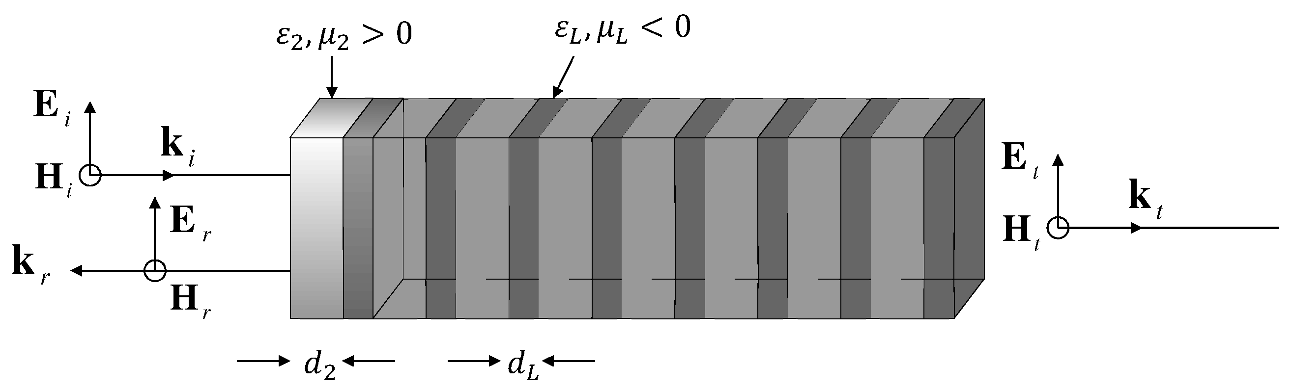
We will now calculate the transmission coefficient through a metamaterial superlattice
with
n unit cells bounded by semi-infinite air layers, for the unit cell parameters indicated in
Figure 7. The transmission amplitude
through the structure
is given by [
25]:
where
is the element
of the transfer matrix that connects electromagnetic fields at the left- and right-hand sides of the
structure. Assuming
, this matrix element is [
26]:
Here,
,
,
, and
are the real and imaginary parts of the matrix elements of the
n cell (superlattice) transfer matrix
.
, and
,
and
are the real and imaginary parts of the matrix elements:
and:
of the single-cell transfer matrix
M. As mentioned before,
is the Chebyshev polynomial of the second kind and order
n, evaluated at the real part of
.
In
Figure 8, we have the transmission coefficients for two superlattices:
and
, with the same parameters except for the signs of the refraction indices
and
. For the upper panel, we have
n = 6,
,
,
nm,
nm. For the lower panel, we have
n = 6,
,
and
nm, and
nm. As for the metallic superlattice, the transmittance has a band structure; however, at variance with the metallic superlattices, there is no threshold frequency.
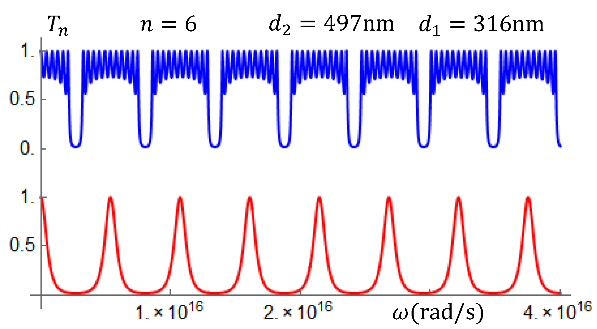
In the left-handed superlattices, an interesting property appears when the well-known
relation for the layers’ widths is considered. If we choose the widths such that
nm, the transmission coefficients become as shown in
Figure 9. In the upper panel a periodic band structure for the superlattice
, while in the lower panel, a collapse of the band structure into a periodic sequence of isolated peaks, for the superlattice
with the
relation in the layers’ widths.
In this particular relation of the left-handed superlattices, where
, also the phase time becomes a periodic function of
with negative values at and around the resonant frequencies see
Figure 10a. We will now build a wave packet (WP), with centroid at one peak of the resonant transmission in
Figure 10a, that will move through the
SL (see the Gaussian envelope in
Figure 10b). We will see the behavior of the the packet components with frequencies around the centroid, whose tunneling times are negative and transmission probabilities close to 1. The predicted tunneling time of the wave-packet peak through the SL with length
, is
fs, and the space-time evolution is as shown in
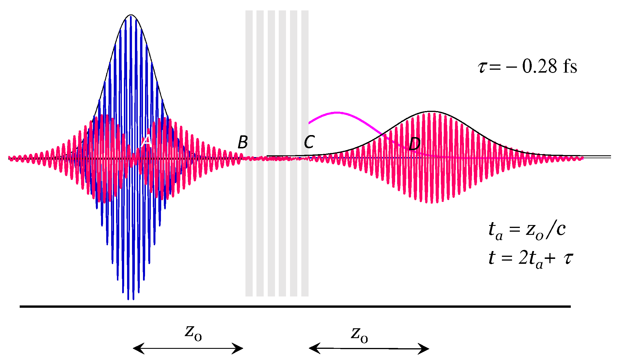
Figure 11.
The snapshots of the theoretical simulation copied in
Figure 11 show the WP at
(blue curve), with centroid at
. This WP moving with group velocity
, arrives at point
B at
.154 fs. If the WP were to move inside the SL with the same velocity
, its peak would reach the point
C at
.44 fs and the point
D at
.60 fs. However, that does not happen. Plotting the space-time evolution of the WP, we see that it reaches the point
D, as predicted, at
.02 fs. The (red) WPs are the partially transmitted and partially reflected. What happens? Do we have an antimatter effect? This result confirms only negative tunneling times. The characteristics of the reflected and transmitted wave packets depend on the frequencies of the components of the wave packet. Wave-packet components near the centroid, with larger transmission coefficients, are transmitted while those in the tails are reflected.
In these systems, as in the metallic superlattices, the dispersion relation is also behind the resonant band structure. Indeed, in
Appendix B, we consider other left-handed SLs with special relations between the layers’ widths and show, for each of these cases, the close relation between the resonant band structure of the transmission coefficient and the dispersion relation in Equation (
23). As shown in
Appendix B, both the Kramer condition and the resonant dispersion relation predict that the bandwidth reduces to one point, when the frequencies fulfill the equation:
Here
is the real part of the matrix element given in (
30). The phase time behavior for MMSLs depends on many factors. Different Gaussian packets with centroids at qualitatively different frequency domains will have also different space-time evolutions.


