Statistical Assessment of Open Optical Networks

Abstract

In order to cope with the increase of the final user traffic, operators and vendors are pushing towards physical layer aware networking as a way to maximize the network capacity. To this aim, optical networks are becoming more and more open by exposing physical parameters enabling fast and reliable estimation of the lightpath quality of transmission. This comes in handy not only from the point of view of the planning and managing of the optical paths but also on a more general picture of the whole optical network performance. In this work, the Statistical Network Assessment Process (SNAP) is presented. SNAP is an algorithm allowing for estimating different network metrics such as blocking probability or link saturation, by generating traffic requests on a graph abstraction of the physical layer. Being aware of the physical layer parameters and transceiver technologies enables assessing their impact on high level network figures of merit. Together with a detailed description of the algorithm, we present a comprehensive review of several results on the networking impact of multirate transceivers, flex-grid spectral allocation as a means to finely exploit lightpath capacity and of different Space Division Multiplexing (SDM) solutions.

1. Introduction

The IP traffic forecasts [1] show that the final user will rule the traffic increase. The drawing forces of this trend are the extensive diffusion of personal data sharing applications and multimedia applications, such as video streaming, enabled by the development broadband access technologies. Such a scenario will strongly change the traffic model for core networks as it will become more and more unpredictable and fluctuating. On the other hand, telecommunications operators aim to continue exploiting the already installed equipment at least until 2025 [2] because of the large CAPEX investments on fiber links done at the beginning of the 2000s [2]. In this context, it is crucial to maximize the capacity deriving from the physical layer enabling flexible network loading [3]. To pursue such results, an accurate assessment of potentialities and criticalities of the network physical layer is an indispensable request.

This leads to the need for defining and evaluating metrics for the performance evaluation of the whole optical network, rather than focusing only on the quality of transmission (QoT) of the point-to-point optical link. In addition, the availability of flexible transponders, whose rate can be adapted based on the available QoT, makes room for a lot of optimizations in the context of the elastic paradigm implementation in Dense Wavelength Division Multiplexing (DWDM) systems networks [4]. These optimizations enable to finer tune the average traffic an optical network can support. The delivered traffic on a given physical topology and transponder technology can be thus considered as a network performance metric. In addition, another higher level network performance metric can be linked to the probability that a connection request between two nodes of the network is accepted or refused. Hence, in the planning and managing of an optical network, it is crucial to foresee the blocking probability of a connection request, given certain traffic conditions. In both cases, the awareness of the physical layer of the network is a key feature to provide reliable performance metrics estimations aimed at the planning, upgrade and orchestration of an optical network.

In this paper, we review several studies on the physical layer impacts on the network performance. To perform the aforementioned studies, we propose what we call a Statistical Network Assessment Process (SNAP). This methodology is based on the waveplane-based routing and wavelength assignment (RWA) [5,6] and performs a loading of the network through a Monte Carlo algorithm (MCA) [7] in which at each iteration corresponds to a different realization of the set of lightpath (LP) allocation requests. The set of traffic requests between two nodes of the network can be finite and given a priori or the network can be progressively loaded generating data connection requests according to a certain probability distribution until a stop criterion. Furthermore, SNAP is able to work on topologies completely unloaded or partially loaded by pre-existing legacy traffic.

In our analysis, we consider as propagation impairments the amplified spontaneous emission (ASE) noise generated by the optical amplifiers and the fiber nonlinear propagation effects treated as a noise-like disturbance called nonlinear interference (NLI). The propagation impairments are directly linked to the physical structure of the network and set its performance through the available QoT of the single LPs [8,9,10,11,12,13,14,15,16,17]. Here, we will always assume networks operating according to the Locally-Optimized-Globally-Optimized (LOGO) strategy [18,19,20], meaning that each link works at its optimum transmitted power [16,21], which minimizes the NLI. Given a description of the network topology and transmission technologies, SNAP is capable of evaluating several metrics such as statistics of the average bit-rate per LP $<R_{b,\lambda }>$ for all possible LP demands arrangement, blocking probability ($BP$) vs. allocated traffic and average load of each link. Such statistical characterization can be used to derive general and statistically effective assessment of the network performance. We remark that suggesting optimal routing and wavelength solutions is out of the scope of this paper. The primary goal of SNAP is the statistical benchmarking of the physical layer to identify strengths and weaknesses under a given- or progressive-traffic loading of networks.

The paper is organized as follows: In Section 2, we give a general overview of how the physical layer can be effectively and efficiently abstracted to the network layer; Section 3 gives an accurate and detailed description of the SNAP algorithm in case the traffic load is given or progressive. In Section 4 and Section 5, we report several results obtained using the given traffic and progressive traffic loading, respectively. In Section 6, we draw some conclusions about our investigation.

2. Network Abstraction in Open Optical Networks

As mentioned earlier, the main goal of SNAP is to provide a tool to statistically evaluate disadvantages and advantages of the physical layer of reconfigurable optical networks. To the present day, the tendency of vendors and operators is to expose the physical characteristics of the network elements together with telemetry data by opening the optical networks. This allows for building software-based reliable estimations of diverse quality of transmission metrics enabling physical layer aware design and management of optical networks. In particular, among the figures of merit, as shown in [22,23], we take into account the signal-to-noise ratio (SNR), which is defined as:

$$\mathrm{SNR}=\frac{P_{ch}}{P_{\mathrm{ASE}}+P_{\mathrm{NLI}}},$$

(1)

where $P_{ch}$ is the channel power, $P_{\mathrm{ASE}}$ is the ASE noise power generated by all the optical amplifier along the path and $P_{\mathrm{NLI}}$ is the overall equivalent NLI power due to the fiber spans.

2.1. From the Physical Layer to the Graph Representation

Starting from Equation (2), it is possible to decompose the overall noise disturbances in the contributions introduced by each Line System (LS) in the network as $P_{\mathrm{ASE}, \mathrm{LS}}$ and $P_{\mathrm{NLI}, \mathrm{LS}}$, i.e., the overall ASE noise and NLI introduced by a LS. Here, the LS is intended as the sequence of fibers and amplifiers connecting two adjancent network nodes. It is then possible to get the relation between the overall SNR of a LP and the signal degradation introduced by each LS as follows:

$$\mathrm{SNR}=\frac{P_{ch}}{{\sum }_{LS}{P}_{\mathrm{ASE}, \mathrm{LS}}+P_{\mathrm{NLI}, \mathrm{LS}}}={\left(\sum _{LS}\frac{P_{\mathrm{ASE}, \mathrm{LS}}+P_{\mathrm{NLI}, \mathrm{LS}}}{P_{ch}}\right)}^{-1}={\left(\sum _{LS}iSN{R}_{\mathrm{LS}}\right)}^{-1},$$

(2)

where $iSN{R}_{\mathrm{LS}}$ is the SNR degradation introduced by a LS and it is defined as:

$$iSN{R}_{\mathrm{LS}}=\frac{P_{\mathrm{ASE}, \mathrm{LS}}+P_{\mathrm{NLI}, \mathrm{LS}}}{P_{ch}}.$$

(3)

In such a way, it is possible to estimate the SNR of an optical path in the network just by summing up all the SNR degradation of each LS. The network can be described by graphs whose nodes are the reconfigurable optical add-drop multiplexers (ROADMs) (the network nodes) and the edges are the LSs connecting the network nodes. Hence, given a graph describing the network topology, it is possible to abstract the physical layer just by weighting each edge with the corresponding LS SNR degradation $iSN{R}_{\mathrm{LS}}$, which is evaluated by means of a quality of transmission estimator (QoT-E) module considering the ASE and NLI impairments with proper analytic models. The resulting graph representation can be used to have a quick and accurate estimation of the SNR experienced by a specific LP or to address the routing algorithm. It should be underlined that the weighting can be based on various quality metrics such as the latency. However, in the following investigations, the selected quality metric will always be the SNR degradation.

The main requirement to obtain such physical layer abstraction is that the NLI model in the QoT-E should assume the incoherent accumulation, i.e., a model capable of disjointing the NLI contribution of each fiber span. Another strong requirement is the independence from modulation format used. To do so, we use the incoherent GN (IGN) model [16] to evaluate propagation performances. The IGN model is suitable for physical layer impairment aware networking scenarios within some limitations—e.g., for low span loss. In Section 5.3, we prove the IGN to be sufficiently reliable for networking studies [24] in estimating the NLI efficiency among the available GN model versions [16,18,19,21].

2.2. Routing Strategies

Given the network physical layer abstraction, in general, the routing, spectral and wavelength assignment (RSWA) problem has to be solved according to a certain strategy. This means to assign the optical path and wavelength to a connection request. The spectrum assignment problem is actually solved in case flexible-grid spectral allocation method is used. If fixed-grid is used, only the channel wavelength has to be assigned and we call it simply an RWA problem. Flexible/fixed-grid will be discussed in Section 5. As an RWA strategy, first we compute the routing space and then the wavelength assignment. The routing space is computed using the Dijkstra algorithm [25] on the weighted graph representing the network abstraction. SNAP can make use of several weights such as $iSNR$, the latency, the LS’s length or the number of hops. For each node pair, $k_{MAX}$ shortest paths are computed. Regarding the wavelength assignment, we adopt a modified version of the waveplane method [5], which is based on a multilayer graph made of $N_{\mathrm{ch}}$ planes, called waveplanes, where $N_{\mathrm{ch}}$ is the number of spectral slot ($\lambda$s). In waveplanes, each edge of the graph corresponds to a single $\lambda$ on the corresponding LS. Then, the RWA works as follows:

• For each traffic request, the $k_{MAX}$ shortest paths are explored;
• For each of the selected paths, all the waveplanes are scanned until a suitable working LP to accommodate the request. LP selection is done by considering the weights of the edges of the available optical paths;
• Whenever a demand is allocated, the edges of that waveplane corresponding to the LP are labelled as busy;
• If a request cannot be allocated, it is counted as rejected and the RWA moves to the next request.

The adopted RWA is a first-fit wavelength assignment with routing based on a weighted $k_{MAX}$-shortest-path. Hence, a $k_{MAX}$-best-SNR based routing policy implies that $k_{MAX}$ paths between a pair of nodes with highest SNR are considered as suitable paths for LPs.

3. SNAP: Statistical Network Assessment Process

In this section, we describe in detail the SNAP algorithm. SNAP has been introduced in [24] and used in [7,26,27,28,29,30,31,32,33]. An extensive discussion on the application of SNAP can be also found in [34]. SNAP is an algorithm that carries out statistical benchmarking of reconfigurable optical networks performance with physical layer awareness. The SNAP algorithm is briefly described by means of pseudocode in

Table 1. SNAP algorithm for given traffic and progressive traffic loading.

. SNAP is a Monte Carlo based algorithm whose set of input parameters can be roughly divided in the description of the crude network hardware and in the description of the way we want to feed and use it, as detailed in the following:

• Description of the Network Topology and Physical Layer: a set of network nodes and their relative connectivity matrix describe the network topology. Beyond this logical description, the set of physical parameters describing the hardware composing the network must be provided. For example, a network node could be physically characterized simply as the ROADM loss and the noise figure (NF) of the amplifier recovering its loss or even by a more complex model characterizing its filtering effect. As for the optical fiber links connecting the nodes, we take into account the fiber type (with its physical parameters such as length, attenuation coefficient, dispersion and effective area) and the inline amplifiers NF. This data is then used to estimate the QoT metric of each LP, such as the SNR degradation, via the model of choice [16]. However, note that it is also possible to provide directly the graph and the weights of its edges.
• Spectral Information and Network Management Strategies: This set of parameters describes how the network hardware should be operated. This includes:
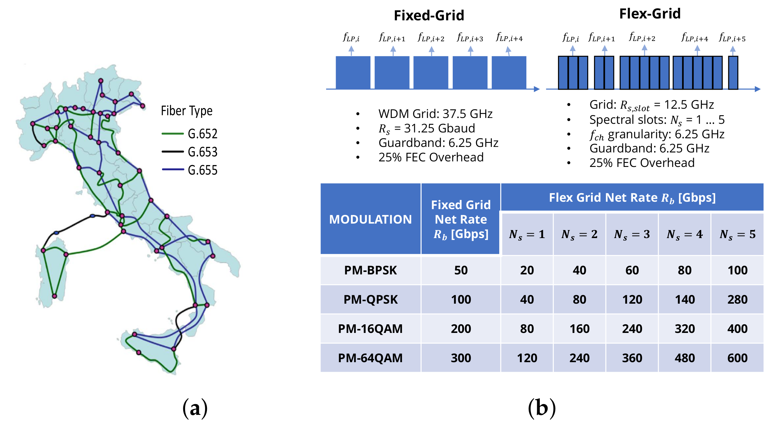
  • Spectral Information: the description of the transceivers generating and receiving the data signals to inject into the network. This involves the used spectral region (C-Band, L-Band, Multiband, etc.), fixed or flexible-grid spectral allocation, grid size, fixed or multi-rate transmission, symbol rate, FEC overhead and pre-FEC target BER;
  • Power Control Plan: this defines the power management strategy used for transmission along the optical paths, such as the LOGO strategy for SNR optimization;
  • Routing and Spectrum/Wavelength Assignment (RSWA) algorithm: This describes how the optical paths between a nodes pairs are evaluated and ranked and spectral slots assigned to LPs, i.e., the routing policy. For example, a shortest link or lowest latency routing could be adopted as well as best-QoT routing.
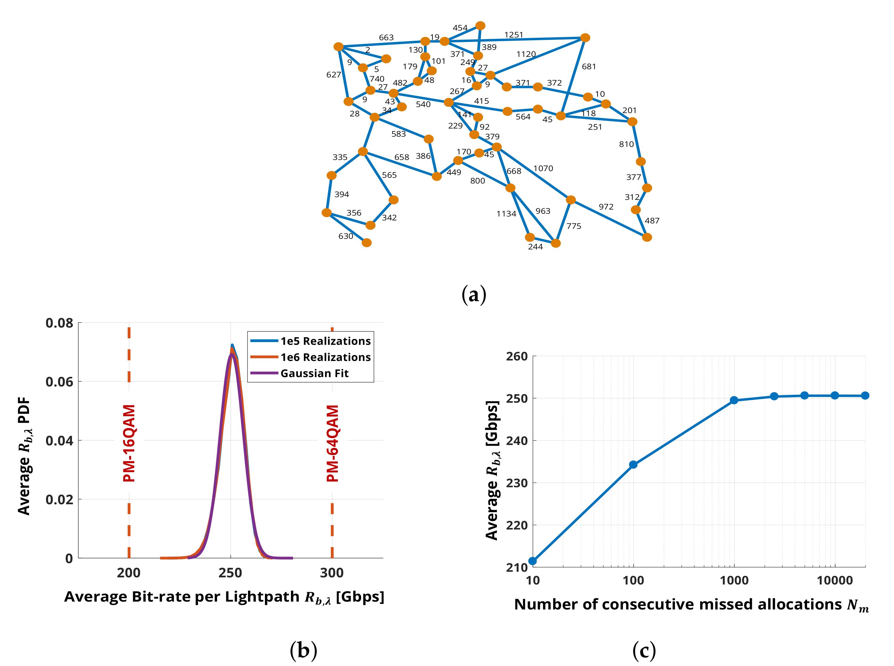
• Traffic Model Description: The traffic loading the network is given as a set of LP allocation requests between two network nodes. In addition, pre-existing legacy traffic loading the network is supported. A certain number of Monte Carlo realizations $N_{MC}$ to run over must be set due to the stochastic nature of the traffic requests in order to provide reliable network statistics. This tuning will be shown once in Section 5.1 by looking at the convergence of the average bit-rate per LP, so that results are indeed probability density functions (PDFs) of targeted metrics. As described in the following, SNAP supports two models for traffic loading, identified as given traffic or progressive traffic analyses.
  • Given Traffic Analysis: as described in the left-side pseudocode of Table 1, we define a traffic matrix D, whose elements $D_{l,m}$ may represent either a connection request or a data-rate request between nodes l and m. In the former case, $D_{l,m}$ represents the number of LPs to be established between nodes l and m. In the latter, it is a transport request between nodes l and m of groomed traffic of size $R_G$ that the physical layer should be fulfilled according to the transceiver technology (fixed- or multi-rate) and spectral allocation strategy (fix- or flex-grid). For example, a D matrix such that $D_{l,m}=1$ ∀ $l,m$ and $D_{l,m}=0$ for $l=m$ represents an any-to-any connectivity case, i.e., each node can request a LP to each of the other nodes except to itself. At each Monte Carlo iteration, the randomness of the LP requests lies in the order in which the $D_{l,m}$ elements are picked up. For each $D_{l,m}$ the algorithm tries to allocate a LP, i.e., a suitable wavelength and optical path according to the RSWA strategy. If the LP allocation is successful, the corresponding bit-rate $R_{b,n}$ is collected, n being the index of the n-th allocated LP at the i-th Monte Carlo iteration. Otherwise, the missed allocation counter is incremented. After all the $D_{l,m}$’s are processed by the RSWA algorithm, the network loading loop terminates, so that the network reaching the saturation state is not assured. Hence, this analysis is aimed at deriving static metrics by looking at the network status after each loading loop. The loading loop is repeated for each Monte Carlo iteration and static metrics are finally calculated from the obtained PDFs.
  • Progressive Traffic Analysis: with respect to the right-side pseudocode of Table 1, in this case, LP alllocation requests are issued indefinitely with the progressive loading loop on i-th Monte-Carlo iteration. Traffic requests $D_{l,m}$ are generated according to a probability mass function in the space of the source/destination nodes, expressing the probability that a connection request between nodes $l,m$ might occur. In SNAP, we assume that this probability distribution is uniform among the nodes at each iteration i, so that the connection request probability is equal to $1/\left[N_{\mathrm{nodes}}(N_{\mathrm{nodes}}-1)\right]$ and constant for each nodes pair, $N_{\mathrm{nodes}}$ being the number of network nodes generating and receiving traffic. As for the given traffic case, LP allocation requests can be either connection requests or data-rate requests. In turn, the grooming size $R_G$ can be fixed and defined at the logical level or generated from a certain probability distribution. Similarly to the given traffic case, if an LP can be allocated for the issued $D_{l,m}$ request, the corresponding bit-rate $R_{b,n}$ is calculated; otherwise, the missed allocation counter is incremented. Here, however, the network loading loop terminates at network saturation, i.e., when $N_m$ subsequent requests for connections are blocked. Hence, progressive traffic analysis is suitable for both static and dynamic metrics estimation, since statistics at a certain network load level or at network saturation can be obtained. The loading loop is repeated $N_{MC}$ times and, in the end, performance metrics are obtained from the obtained PDFs.

As previously mentioned, the SNAP algorithm generates a different random realization of the network load evolution at every i-th iteration of the MCA; then, the average bit-rate per LP $R_{b,\lambda }^i$ is computed by averaging over the bit-rates achieved by each allocated LP as follows:

$$R_{b,\lambda }^i=\frac{1}{N_{L,i}}\sum _{n=1}^{N_{L,i}}{R}_{b,n}\left[\mathrm{Gbps}\right],$$

(4)

where $N_{L,i}$ is the number of allocated LPs during the i-th Monte Carlo run and $R_{b,n}$ is the bit-rate of the n-th allocated LP.

For both given and progressive-traffic analyses, several networks metrics can be computed and stored at each i-th Monte Carlo run. This can be generalized to different performance metrics. Thus, it is possible to investigate:

• Average bit-rate per LP$R_{b,\lambda }^i$ of Equation (4);
• Spectral saturation: the spectral occupation of each node-to-node fiber connection;
• Blocking information: the number of blocked demands for each node or link;
• Acceptance information: the number of demands accepted in each node.

Alternatively, network statistics versus the loading evolution can be calculated, thus obtaining dynamic metrics of the network conditions:

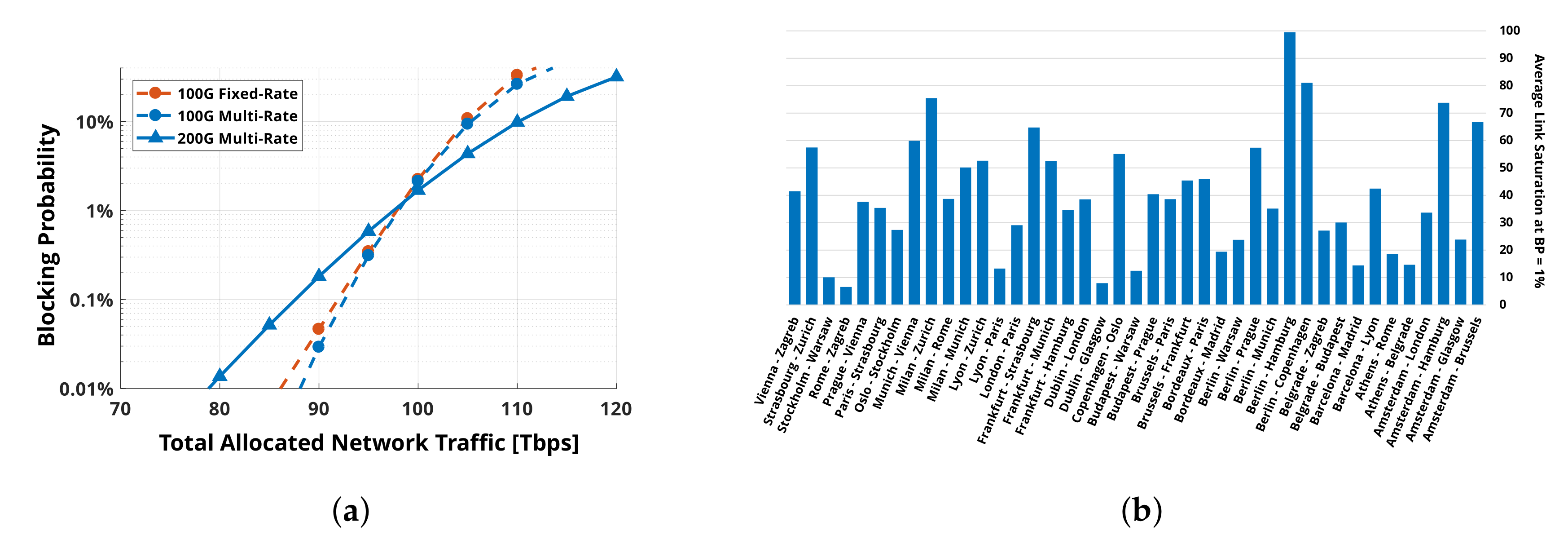
• Blocking Probability: the probability of demand $j+1$ being blocked after demand j. $BP$ can be considered the Quality-of-Service (QoS) figure of merit of the network under progressive loading;
• Total allocated network traffic: obtained as the sum of the number of allocated LP requests up to the j-th demand. Selecting a target QoS, one can evaluate the average maximum traffic supported by the network at that target QoS;
• Link saturation: the number of the allocated LPs in the overall available bandwidth in each network link.

It is worth noting that the two network loading strategies presented here come in handy for different use cases. Given traffic loading provides static network metrics. The metrics are static in the sense that they are useful when we we want to study the network performance in a steady state where it is loaded with a fixed and known traffic and not pushed to its saturation limits. Conversely, progressive traffic loading delivers dynamic metrics, in the sense that they allow us to look at the evolution of the statistical performance of the network, such as the total allocated capacity, without having any knowledge of the actual traffic matrix. The capacity is then evaluated as the network is loaded with increasing traffic in time and can be thus linked to a certain $BP$.

As for the RSWA algorithm, here we will always adopt a first-fit wavelength assignment with a $k_{MAX}$-best-SNR based routing policy. It is worth noting that, while we are aware that it is not the optimal strategy, it is still possible to implement diverse RSWA strategies following the pseudocode in Table 1 in order to conduct further studies in order to assess the impact of different algorithms on network performance. For example, progressive traffic loading could be employed in order to estimate the gains and losses in network capacity vs. $BP$ passing from standard first-fit wavelength assignment to more sophisticated approaches.

4. Given Traffic Results

As a first SNAP analysis, we review the results presented in [7]. Here, we have derived the average bit-rate per LP $<R_{b,\lambda }>$ by means of given-traffic investigation as static metric for the network physical layer. Here, we have compared the networking figure of merit of the three typical fiber types of

Table 2. Physical parameters of PSCF, SMF and NZDSF fiber types considered.

Fiber Type	Loss ${\mathit{\alpha }}_{\mathbf{dB}}$ [dB/km]	Dispersion D [ps/(nm · km)]	Effective Area ${\mathit{A}}_{\mathbf{eff}}$ [$\mathsf{\mu }$m${}^2$]
NZDSF	0.220	3.8	70
SMF	0.200	16.7	80
PSCF	0.167	21.0	135

, together with the adoption of multi-rate transceiver based hybrid and pure modulation formats. The analysis has been done on the Pan-EU COST network depicted in Figure 1a. An any-to-any connectivity matrix has been considered as a traffic model with $k_{MAX}$-best-SNR based routing policy Section 3. We have heuristically estimated that $N_{MC}=5000$ Monte Carlo runs are needed to obtain a reliable network statistics estimation. The $<R_{b,\lambda }>$ obtained averaging the PDF of the lightpath rates obtained by the MCA is adopted as a unique static network performance metric. The multi-rate transceiver based on pure modulation formats, i.e., polarization multiplexed-quadrature amplitude modulation of cardinality M (PM M-QAM) constellations, delivers a finite and discrete set of rates, determined by the maximum cardinality of the constellation M supported by the available QoT of the selected LP. On the other hand, the hybrid multi-rate transceiver exploits Time Division Hybrid Modulation Formats (TDHMFs) [35,36], enabling adjusting with continuity the delivered rate to the available QoT of the considered LP. For both options, we assume to employ only on modulation formats with squared constellations, (PM-BPSK, PM-QPSK, PM-16-QAM, PM-64-QAM), where data flows of the four quadratures are independent. Hence, for pure modulation formats, the spectral efficiency varies in the discrete set of $[2,4,8,12]$ bit per symbol (BpS) according to the QoT and corresponding to a delivered net bit-rate of $[50,100,200,300]$ Gbps. TDHMF transceivers instead allow for adapting the BpS with continuity from 2 to 12 and to tune their rate from 50 to 300 Gbps, depending on the SNR degradation of the selected LP. On the digital signal processing (DSP) side units, we assume to manage a gross data symbol rate $R_{s,g}=32$ GBaud per LP, corresponding to a net symbol rate $R_s=25$ GBaud per LP due to protocol and Forward Error Correction (FEC) overhead assumed to be of 28%. Thus, LPs are assumed in-service on the selected paths if the pre-FEC BER $\le 4\times {10}^{-3}$, then the transceiver rate is scaled accordingly with the given SNR [36]. For each fiber-type, Figure 1b shows the average $R_{b,\lambda }$ enabled by PM-M-QAM and TDHMF obtained for the COST topology.

As for the merit of fiber types, the performance hierarchy observed for point-to-point transmission [21] is still valid at the network level: for both transceiver technologies, the best-performing PSCF is followed by SMF and NZDSF, with the NZDSF always showing nearly a 30% of rate penalty with respect to SMF due to the small dispersion and effective area enhancing nonlinear effects. Comparing the two options for multi-rate transceivers, TDHMF provides always better performance than PM-M-QAM. Its relative $<R_{b,\lambda }>$ advantage over PM-M-QAM is 20%, 26%, 28% with PSCF, SMF, NZDSF, respectively. This advantage is explained by the capability of TDHMF to exploit the available QoT more effectively when the physical layer does not allow for achieving the maximum rate because of the poor quality of the fibers in larger networks. In a more general picture, these first results show how SNAP can be employed to push further the capacity of the optical network by planning transponder upgrades to flexible transponders in topologies offering low QoT paths.

5. Progressive Traffic Results

In this section, we review the results obtained loading the network with progressive traffic. First, in Section 5.1, we show some preliminary results on the convergence of the MCA [7,28] and we review the general impact of NLI as previously approached in [28] in Section 5.2. Afterwards, in Section 5.3, we compare the average $R_{b,\lambda }$ per LP obtained by using a QoT-E based on three different models (GN, incoherent-GN (IGN), enhanced-GN (EGN) [37]) for the physical layer impairment evaluation taking into account fixed and multi-rate transceivers as already presented in [24]. In Section 5.4, we reexamine the work of [26] presenting further results on the fixed and hybrid rate transceivers impact. Then, we revise [29] on the effects of fixed and flexible grid as spectral allocation methods in Section 5.5 and as a final study, in Section 5.6, the benefits of different SDM solutions have been reviewed as done in [31].

5.1. Preliminary Results on SNAP Algorithm Convergence

As a first investigation, we have tested SNAP in progressive traffic loading on the Pan European network topology [24] of the EU project “IDEALIST” [38] depicted in Figure 2a. Links are assumed to be uniform in terms of fiber and erbium doped fiber amplifier (EDFA) types. As fiber pairs, we consider SMF parameters as in Table 2, with nonlinear index coefficient $n_2=2.5\times {10}^{\ast 20}{\mathrm{m}}^2/\mathrm{W}$ corresponding to a nonlinear coefficient $\gamma =1.27$ 1/W/km. ROADMs are assumed to introduce 10 dB of routing loss fully recovered by an EDFA with 5 dB of noise figure at the node output without any further filtering impairment. Span lengths are not uniform and they are obtained from the topology data in [38]. On the transmitter level, we transmit a maximum of $N_{\mathrm{ch}}=80$ LP (wavelengths) per fiber over the 4 THz of C-Band on the 50 GHz ITU-T grid. As in Section 4, flexible-rate transponders based on pure PM-M-QAM or on TDHMFs are adopted and operating at the same gross symbol rate $R_{s,g}$, net symbol rate $R_s$ and pre-FEC BER. First, the convergence of the MCA, i.e., the number of Monte Carlo iterations $N_{MC}$ needed to obtain statistically stable results, has been verified. To this aim, the PDF of the average bit-rate per LP given by Equation (4) obtained with $N_{MC}={10}^5$ and $N_{MC}={10}^6$ has been estimated. As for the routing policy, we set $k_{MAX}$-best-SNR with $k_{MAX}=4$. PDFs are reported in Figure 2b together with a Gaussian fit for TDHMF. Due to the central limit theorem, the average $R_{b,\lambda }$ PDF converges towards the Gaussian distribution with respect to the LP allocations, so its average value can be used as a figure of merit in the comparison of different implementations of the physical layer. This can be explained with the fact that $R_{b,\lambda }$ is in fact computed as a sum from a large set of random bit-rates, whose stochasticity is mainly caused by network blocking and routing strategy. Hence, increasing $k_{MAX}$, i.e., exploring a larger routing space; thus, expanding the variability of the allocation process leads to the increase of the $R_{b,\lambda }$ variance. It can be observed that, for $N_{MC}={10}^5$, the algorithm has already converged since the curves perfectly match. Moreover, independently from the LP allocation order, the considered network topology delivers nearly 250 Gbps per LP on average. This means 5 BpS per polarization, larger than the 4 BpS of a pure PM-16-QAM. In addition to the $R_{b,\lambda }$ PDF, we report in Figure 2c the average bit-rate per LP $<R_{b,\lambda }>$ versus the number of missed allocations $N_m$ required to stop the Monte Carlo iteration at $N_{MC}={10}^5$. The resulting $<R_{b,\lambda }>$ saturates from $N_m\ge 2000$. In light of this evidence, we safely set $N_{MC}={10}^5$ and $N_m=5000$ to obtain the results presented in the next section.

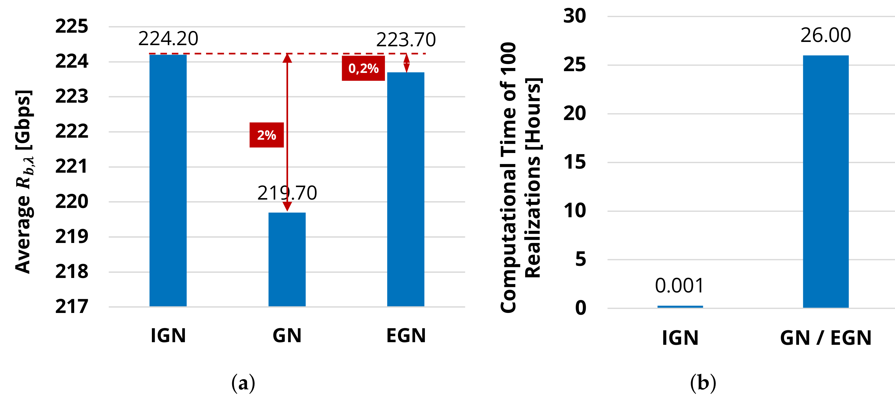
5.2. Network NLI Penalty Assessment with Pure/Hybrid Modulation Formats

Once calibrated $N_{MC}$ for SNAP to converge, we evaluated the impact of nonlinearities on the average bit-rate per LP that the IDEALIST network of Section 5.1 can support [24]. With such a purpose, we set the transmitted power per channel on each link $P_{\mathrm{ch}}$ to:

$$P_{\mathrm{ch}}=P_{\mathrm{ch},\mathrm{opt}}+\Delta PdBm,$$

(5)

being the power offset $\Delta P\in [-3,+3]$ dB. $P_{ch,opt}$ is the optimized launch power per span according to the LOGO principle by means of IGN model. Further investigations on the nonlinear modeling are presented in the next subsection. Each Monte Carlo analysis was performed both including the NLI effect and excluding it by setting $P_{NLI,LS}=0$ to zero in Equation (3). Figure 3 reports $<R_{b,\lambda }>$ versus $\Delta P$ for each of the two modulation strategies, both considering and neglecting NLI, with $k_{MAX}=4$. The pure-format curves displays an $<R_{b,\lambda }>=224$ Gbps at optimum launch power, while TDHMF has a 12% advantage allowing to reach $<R_{b,\lambda }>=250.6$ Gbps as already shown in Figure 2b. As previously explained in Section 4, the considerable TDHMF advantage is due to its ability to better exploit the available SNR on LPs, at the cost of an increased complexity of the DSP, i.e., an increased CAPEX for node equipment. Although elastic, the pure format approach allows a coarse granularity in SNR vs. BpS. In fact, to move from PM-QPSK to PM-16-QAM [39], nearly 6 dB of SNR increase is required. For comparison, the graph also shows what happens when neglecting NLI, showing that $<R_{b,\lambda }>$ tends to saturate at the maximum possible rate $R_{b,\lambda }=300$ Gbps, corresponding to the use of PM-64-QAM on all LPs. Neglecting NLI would thus overestimate $<R_{b,\lambda }>$ of 8% at the optimum power, but this error would grow up to 20% if we operate at $\Delta P=+1$ dB. These results have shown that an accurate estimation of the NLI is necessary since inaccuracies in the QoT lead to substantial under/overestimation of the network capacity metric.

5.3. QoT-E Layer Analysis

As shown in Section 5.2, NLI estimation in the QoT-E layer of SNAP is a crucial point when evaluating network capacity. There, NLI estimation was accomplished using the IGN model, which has been proved to deliver accurate and reliable results [23]. However, different versions of the model exist in literature trading off between accuracy and computational complexity.

In this section, we have compared the network metrics obtained in Section 5.2 by using the IGN with other versions of the model [24]. Given the set of LPs allocated using the IGN model in Section 5.2, we re-evaluated the LP SNR and the corresponding $R_{b,\lambda }$ also using the coherent GN model [40]. Moreover, for the pure modulation format case, we evaluated also the correction factor required by the EGN model, which is considered to be the most accurate version among the so-called GN based models [37].

Using the NLI efficiency obtained with the GN and EGN models, we re-evaluated the SNR for each LP and re-assigned the corresponding $R_{b,\lambda }$. Due to the high computational effort needed to evaluate NLI efficiency using GN and EGN models, such a process was performed only for the first 100 Monte Carlo realizations. The computation required around 26 h using a 12-core CPU, to be compared with the approximately 3 s needed on the same machine using the IGN model (Figure 4b). In Figure 4a, we report the resulting $<R_{b,\lambda }>$ for the pure format approach for the three different NLI models with the performance loss for coherent GN and EGN model with respect to the IGN model. As the GN model overestimates NLI with respect to the IGN, a lower $<R_{b,\lambda }>$ is obtained for GN. The EGN model instead yields, as expected, results that are closely comparable with the IGN ones. In particular, by using a GN model, $<R_{b,\lambda }>$ is estimated to be around 2% smaller than the one obtained with IGN. For EGN, this loss reduces to less than 0.2%, thus the similarity between GN and EGN model is evident. However, it is worth noting that the NLI efficiency has been re-obtained with GN and EGN a posteriori. Other than not computationally convenient, these models could not be used in real time because they lack the incoherent accumulation over fiber spans, which has been assumed in Section 2.

5.4. Network Impact of Fixed and Hybrid Rate Transceivers

In this section, we present the results obtained with the SNAP algorithm by progressively loading with traffic the Pan-EU COST network [26] of Figure 1, where node-to-node links were assumed to be uniform and made of amplified SMF fiber pairs. Here, we targeted the estimation of the dynamic metrics already mentioned in Section 3 such as $BP$ and Link saturation. While in the previous results the traffic requests were exploiting the whole capacity offered by the optical path, here we load the network with data-rate requests between a node pair with grooming size $R_G$, of 100 Gbps or 200 Gbps. We have compared the performance delivered by the two grooming rates $R_G$ together with the the merit of a multi-rate transceiver based either on PM-M-QAM pure modulation formats and a fixed-rate transceivers based on PM-QPSK and PM-16-QAM, delivering respectively 100 Gbps and 200 Gbps per LP. Pre-FEC BER has been set to $4\times {10}^{-3}$ as in Section 4. We assume that the multi-rate transceiver is able to split the traffic on two or more LPs when the available LPs’ QoT is not enough to meet the considered traffic-grooming size. In order to observe performance down to a $BP$ of 0.1%, $N_{MC}={10}^4$ was estimated to deliver sufficiently accurate dynamic metrics. As exit conditions from the network loading loop, we set $N_m$ to be greater than the 50% of the total requests, with a minimum of 5000 generated requests.

The behavior of $BP$ vs. the average total allocated network traffic for both grooming values and transceivers technologies is shown in Figure 5a. The $BP$always grows as the network is progressively loaded with random requests. However, the $R_G=200$ Gbps/fixed-rate transceiver curve is not shown since a very small fraction of LPs had enough QoT to enable PM-16-QAM transmission, leading to large $BP$, larger than 50%, even for limited traffic. Looking at the curves, we can identify two regimes vs. $BP$. For $BP$ below 1%, 100 Gbps grooming always performs better than 200 Gbps grooming. At low $BP$, the large unoccupied wavelength availability makes the LP assignment dominated by the QoT, while 200 Gbps requests are more likely to be blocked because of their larger SNR requirements. Above $BP$ of 1%, the ranking is reversed with 200 Gbps grooming delivering larger throughput. Now, an LP request is more likely to be blocked due to the lack of wavelengths instead of its QoT constraint. However, 200 Gbps requests carry twice the traffic of the 100 Gbps requests, thus resulting in a larger allocated traffic and reversing the ranking. In addition, Figure 5b shows the average saturation for $R_G=200$ Gbps and multi-rate transceivers with bars for each link of the Pan-EU network. Here, we have obtained the static metric at QoS-BP of 1%, but the dynamic link saturation vs. the network loading can be easily obtained from SNAP. Here we can observe some critical facts about the network. The shorter links of the northern area connecting Hamburg, Amsterdam, Berlin and Copenhagen are more congested since they carry a large amount of traffic, while the most peripheral links are less used do to their larger SNR degradation, thus they should be improved at the physical layer. These kind of studies allow for unveiling crucial aspects on the effect of physical layer on networking performances, enabling physical layer-driven network upgrade and design strategies. See [26], where some possible upgrades derived from these progressive-traffic analyses are presented.

5.5. Fixed vs. Flexible Frequency Grid Comparison

In this section, we use SNAP to evaluate metrics for networks already partially loaded by LP to satisfy legacy traffic demands and compare the performance of fixed and flexible frequency grids as spectral allocation methods to exploit the residual bandwidth for future requests. Legacy traffic is assumed to be spectrally distributed in the 4 THz C-Band so that available residual bandwidth is a continuum. Here, the Italian network depicted in Figure 6a has been analyzed. The topology is composed of G.652, G.653 and G.655 amplified fiber pairs. In addition, 18 dB of loss introduced by ROADMs are compensated by an EDFA with 5 dB of NF at each node output. We consider as residual bandwidth percentage ($RBP)\in [75\%,50\%,25\%]$ with respect to the total bandwidth. The residual bandwidth is employed using multi-rate transceivers with pure modulation formats on the 37.5 GHz grid for fixed-grid approach and a maximum of 5 ITU-T spectral slots per LP 12.5 GHz wide for flex-grid, as summarized in Figure 6b. We have carried out MCA with $N_{MC}=5000$ realizations. For each realization, residual spectrum is progressively loaded with given grooming sizes $R_G\in [20,40,100]$ Gbps. We use a $k_{MAX}$-best-SNR routing up to $k_{MAX}=50$ and LOGO as control plan. Furthermore, here we perform bitrate overprovisioning: when a LP is assigned, if the requested grooming size $R_G$ is smaller than the available rate $R_{b,\lambda }$ of the LP, the residual capacity $(R_{b,\lambda }-R_G)$ is left for future requests. The figure of merit considered here is the BP against the overall allocated traffic per spectral unit (T). T has dimensions (BpS/Hz), thus representing the spectral efficiency, enabling a fair ranking for fix-/flex-grid spectral allocations methods in the considered scenarios. Figure 7 always shows a flex-grid gain over fix-grid, but it decreases at larger grooming rates. In fact, when $R_G$ gets bigger, a LP occupies a larger spectral region comparable to the fixed-grid approach. In this case, the flex-grid advantage occurs on LP with larger QoT for which high cardinality modulation formats, such as PM-16QAM and PM-64QAM can be employed to carry the groomed traffic in fewer slots. Moreover, the $BP$shows two regimes against T: in the first phase; LP allocations saturate the residual bandwidth so that the $BP$ increases rapidly; then, it grows slower because further requests are allocated exploiting bit-rate overprovisioning. The $BP$ threshold for the regime change grows with the grooming size because the residual bandwidth for overprovisioning is consumed faster, while it gets smaller at larger $RBP$ because the use of overprovisioning triggers later. It is in any case smaller for the flex-grid method because of the more efficient use of the bandwidth allowing for allocating more lightpaths.

In Figure 8, we targeted the normalized network traffic at a maximum acceptable blocking probability $B{P}_{max}=1\%$, similarly as in [41]. Trivially, Talways grows with $RBP$, with a larger increment of the flex-grid approach, which exploits more efficiently the larger available bandwidth. At $R_G=20$ Gbps grooming (Figure 7c), the flex-to-fix gain is in fact 2.5 at 25% $RBP$and enlarges to 3.3 for $RBP$ of 75%. Going to larger grooming rates increases the absolute traffic but limits the flex-to-fix gain because of network saturation. At $R_G=40$ Gbps (Figure 7d), grooming the flex-to-fix gain is constant to 2.5 for each $RBP$and saturates to nearly 1.3 at 100 Gbps grooming for all $RBP$. Hence, while the absolute traffic for fixed-grid increases with the same ratio of the increasing grooming sizes, the flex-grid approach is instead limited by saturation but exploiting smaller grooming rates more efficiently.

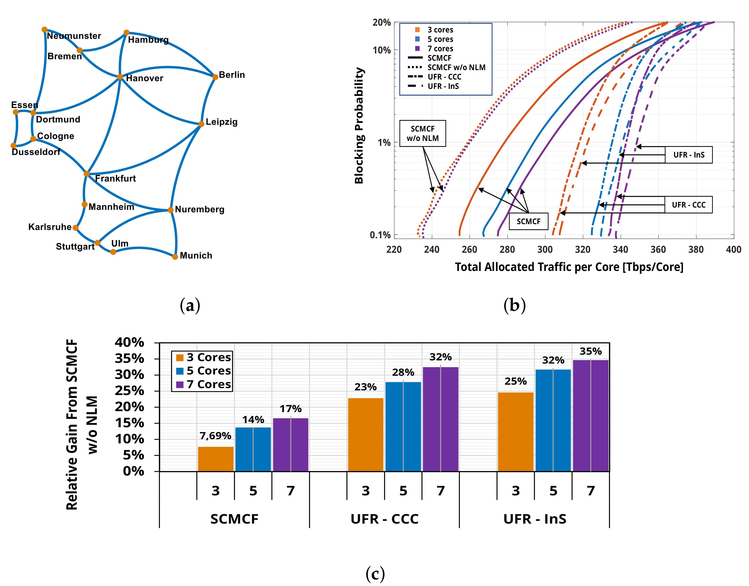
5.6. Networking with Different SDM Solutions

In order to cope with continuously growing capacity demand, a lot of effort has been put on SDM solutions investigations [3,42]. In this section, we use SNAP to evaluate the networking performances delivered by different SDM techniques. As SDM techniques, here we will compare the uncoupled fiber ribbons (UFR) and the strongly coupled multi-core fibers (SCMCF) together with several switching techniques for them [43].

UFRs are considered simply as a set of independent SMF whose nonlinear impairments are the same of single SMF and where independent switching (InS) [44] can be implemented. Here, however, we will apply the core continuity constraint (CCC) [45] switching technique also in UFRs. In SCMCF, the strong coupling between the cores enables nonlinear distortion mitigation (NLM) of the signal, thus improving the SNR and providing point-to-point capacity gain [46,47] when comparing to UFRs with the same SDM cardinality, i.e., number of fibers equal to the number of cores. The SNR improvement from NLM $\Delta SNR$ is derived according to the theory as [47]. However, SCMCFs require joint switching (JoS) implementation [44] due to the strong core coupling. This means that the add/drop of a channel and the LP allocation on a particular wavelength must be done on the same route and in all the cores [46,47]. Hence, while SCMCFs improve QoT, the need for JoS requires the implementation of advanced techniques of routing for space and spectrum assignment (RSSA) [44]; it reduces the total allocated traffic at a given $BP$ [48]. Here, we do not consider advanced RSSA algorithms; we study only the NLM and switching techniques impact instead. From the fiber side, UFRs and SCMCFs have the typical SMF parameters as in Table 2. Span is 100 km, whose loss is recovered by EDFAs with 5 dB of NF. In addition, 18 dB of ROADM loss at each node is recovered by an addition EDFA with 6.2 dB NF. We rely on flexible TDHMF transceivers transmitting up to $N_{ch}=96$ channels per fiber per core in the 50 GHz fixed grid, able to adapt their bit-rate $R_{b,\lambda }$ continuously vs. the SNR. The symbol rate is $R_s=32$ 32 Gbaud, FEC overhead is 28%, and pre-FEC target BER is set to $4\times {10}^{-3}$. Control plan is set to the LOGO strategy. RSWA adopts first fit principle for spatial assignment and $k_{MAX}$-best-SNR strategy with $k_{MAX}=25$ for routing, thus enhancing path diversity and mitigate wavelength contention. We also perform bitrate overprovisioning as in Section 5.5. SNR degradation is evaluated according to the IGN model and full spectral load. The analysis has been carried out on the German topology of Figure 8a by using SNAP with $N_{MC}=$25,000 realizations.

Traffic requests are generated from an any-to-any uniform distribution. SDM solutions are compared at their optimum grooming rate better fitting the physical layer QoT and maximizing the $BP$ vs. total allocated traffic. Varying the SDM cardinality in $[3,5,7]$, we have considered the following combinations of SDM and switching techniques:

• UFR with CCC,
• UFR with InS,
• SCMCF with JoS and NLM,
• SCMCF with JoS and without NLM.

The last one is equivalent to an uncoupled crosstalk-free multicore fiber with JoS. As the network is loaded, we calculate the total allocated traffic normalized to the SDM cardinality, i.e., divided by the number of cores, in order to obtain a fair comparison between the SDM solutions and switching techniques. Figure 8b show the $BP$ against the total allocated traffic per core. The overlapping of the SCMCF w/o NLM curves implies that JoS has no effect in the capacity per core varying the SDM cardinality. All the other cases, instead, show significant performance gains increasing the SDM cardinality, enabled by NLM for SCMCF and by the switching flexibility allowed by CCC and InS for UFRs. However, the cardinality gain slows down passing from five to seven cores and, for low to moderate $BP$, the NLM-enabled enhancement cannot cope with the flexibility offered by UFRs with InS and CCC. Focusing on the UFR switching techniques, the less restrictive InS shows a gap of 1.35%, 1.7% and 1.7% with respect to CCC for three, five and seven cores, respectively. As a static metric targeting $BP={10}^{-2}$, we have reported as vertical bars in Figure 8c; the total traffic gain of UFRs and SCMCF with respect to the SCMCF w/o NLM taken as reference. NLM enables a gain 7%, 14% and 17% per core for three, five and seven cores, respectively. However, the gains enabled by UFRs are fairly larger: 23%, 28% and 32% per core in the case of CCC and by 25%, 32%, 35% per core in case of InS. Focusing on UFRs, InS delivers the best performance. However, the CCC penalty with respect to InS is between 1% and 2%, i.e., fairly small. Nevertheless, since InS implementation in ROADMs constitutes a huge complexity cost, the use of UFRs with CCC can be a nice trade-off to optimize network performances.

6. Conclusions

In this work, we have shown how the SNAP algorithm can be a powerful tool to get a network performance estimation with physical layer awareness. We have explained in detail the algorithm workflow and the concept of physical layer abstraction with a graph. After some details on the importance of a proper and convenient QoT estimation, we have presented an extensive set of applications showing how the use of multi-rate or hybrid transceivers impact the network capacity. Furthermore, a comparison between fixed and flexible spectral allocation methods has been done. Finally, the advantages and disadvantages of different SDM solutions have been studied. These results show that SNAP can be used as a handy tool to address the network design and to properly address the network upgrades to improve the overall performances.

References

1. Cisco. Cisco Visual Networking Index: Forecast and Trends, 2017–2022; Technical Report; Cisco: San Jose, CA, USA, 2017. [Google Scholar]
2. Wellbrock, G.; Xia, T.J. How will optical transport deal with future network traffic growth? In Proceedings of the 2014 The European Conference on Optical Communication (ECOC), Cannes, France, 21–25 September 2014. [Google Scholar] [CrossRef]
3. Essiambre, R.J.; Tkach, R.W. Capacity Trends and Limits of Optical Communication Networks. Proc. IEEE 2012, 100, 1035–1055. [Google Scholar] [CrossRef]
4. Zhou, X.; Nelson, L.E.; Magill, P. Rate-adaptable optics for next generation long-haul transport networks. IEEE Commun. Mag. 2013, 51, 41–49. [Google Scholar] [CrossRef]
5. Dai, H.; Li, Y.; Shen, G. Explore Maximal Potential Capacity of WDM Optical Networks Using Time Domain Hybrid Modulation Technique. J. Lightw. Technol. 2015, 33, 3815–3826. [Google Scholar] [CrossRef]
6. Shen, G.; Bose, S.; Cheng, T.; Lu, C.; Chai, T. Efficient heuristic algorithms for light-path routing and wavelength assignment in WDM networks under dynamically varying loads. Comput. Commun. 2001, 24, 364–373. [Google Scholar] [CrossRef]
7. Cantono, M.; Gaudino, R.; Curri, V. Potentialities and Criticalities of Flexible-Rate Transponders in DWDM Networks: A Statistical Approach. J. Opt. Commun. Netw. 2016, 8, A76. [Google Scholar] [CrossRef]
8. Carena, A.; Curri, V.; Bosco, G.; Poggiolini, P.; Forghieri, F. Modeling of the Impact of Nonlinear Propagation Effects in Uncompensated Optical Coherent Transmission Links. J. Lightw. Technol. 2012, 30, 1524–1539. [Google Scholar] [CrossRef]
9. Bononi, A.; Serena, P.; Rossi, N.; Grellier, E.; Vacondio, F. Modeling nonlinearity in coherent transmissions with dominant intrachannel-four-wave-mixing. Opt. Express 2012, 20, 7777. [Google Scholar] [CrossRef] [PubMed]
10. Mecozzi, A.; Essiambre, R.J. Nonlinear Shannon Limit in Pseudolinear Coherent Systems. J. Lightw. Technol. 2012, 30, 2011–2024. [Google Scholar] [CrossRef]
11. Secondini, M.; Forestieri, E. Analytical Fiber-Optic Channel Model in the Presence of Cross-Phase Modulation. IEEE Photon. Technol. Lett. 2012, 24, 2016–2019. [Google Scholar] [CrossRef]
12. Johannisson, P.; Karlsson, M. Perturbation Analysis of Nonlinear Propagation in a Strongly Dispersive Optical Communication System. J. Lightw. Technol. 2013, 31, 1273–1282. [Google Scholar] [CrossRef] [Green Version]
13. Dar, R.; Feder, M.; Mecozzi, A.; Shtaif, M. Properties of nonlinear noise in long, dispersion-uncompensated fiber links. Opt. Express 2013, 21, 25685. [Google Scholar] [CrossRef] [PubMed]
14. Serena, P.; Bononi, A. An Alternative Approach to the Gaussian Noise Model and its System Implications. J. Lightw. Technol. 2013, 31, 3489–3499. [Google Scholar] [CrossRef] [Green Version]
15. Secondini, M.; Forestieri, E.; Prati, G. Achievable Information Rate in Nonlinear WDM Fiber-Optic Systems With Arbitrary Modulation Formats and Dispersion Maps. J. Lightw. Technol. 2013, 31, 3839–3852. [Google Scholar] [CrossRef]
16. Poggiolini, P.; Bosco, G.; Carena, A.; Curri, V.; Jiang, Y.; Forghieri, F. The GN-Model of Fiber Non-Linear Propagation and its Applications. J. Lightw. Technol. 2014, 32, 694–721. [Google Scholar] [CrossRef]
17. Dar, R.; Feder, M.; Mecozzi, A.; Shtaif, M. Accumulation of nonlinear interference noise in fiber-optic systems. Opt. Express 2014, 22, 14199. [Google Scholar] [CrossRef] [PubMed]
18. Poggiolini, P.; Bosco, G.; Carena, A.; Cigliutti, R.; Curri, V.; Forghieri, F.; Pastorelli, R.; Piciaccia, S. The LOGON Strategy for Low-Complexity Control Plane Implementation in New-Generation Flexible Networks. In Proceedings of the Optical Fiber Communication Conference/National Fiber Optic Engineers Conference 2013, Anaheim, CA, USA, 17–21 March 2013. [Google Scholar] [CrossRef]
19. Pastorelli, R.; Bosco, G.; Piciaccia, S.; Forghieri, F. Network Planning Strategies for Next-Generation Flexible Optical Networks. J. Opt. Commun. Netw. 2015, 7, A511. [Google Scholar] [CrossRef]
20. Pastorelli, R. Network Optimization Strategies and Control Plane Impacts. In Proceedings of the 2015 Optical Fiber Communications Conference and Exhibition (OFC), Los Angeles, CA, USA, 22–26 March 2015. [Google Scholar] [CrossRef]
21. Curri, V.; Carena, A.; Arduino, A.; Bosco, G.; Poggiolini, P.; Nespola, A.; Forghieri, F. Design Strategies and Merit of System Parameters for Uniform Uncompensated Links Supporting Nyquist-WDM Transmission. J. Lightw. Technol. 2015, 33, 3921–3932. [Google Scholar] [CrossRef]
22. Kamalov, V.; Cantono, M.; Vusirikala, V.; Jovanovski, L.; Salsi, M.; Pilipetskii, A.; Kovsh Maxim Bolshtyansky, D.; Mohs, G.; Rivera Hartling, E.; Grubb, S.; et al. The subsea fiber as a Shannon channel. In Proceedings of the SubOptic 2019, New Orleans, LA, USA, 8–11 April 2019. [Google Scholar]
23. Filer, M.; Cantono, M.; Ferrari, A.; Grammel, G.; Galimberti, G.; Curri, V. Multi-Vendor Experimental Validation of an Open Source QoT Estimator for Optical Networks. J. Lightw. Technol. 2018, 36, 3073–3082. [Google Scholar] [CrossRef]
24. Cantono, M.; Gaudino, R.; Curri, V. Data-rate figure of merit for physical layer in fixed-grid reconfigurable optical networks. In Proceedings of the 2016 Optical Fiber Communications Conference and Exhibition (OFC), Anaheim, CA, USA, 20–24 March 2016. [Google Scholar] [CrossRef]
25. Dijkstra, E.W. A note on two problems in connexion with graphs. Numer. Math. 1959, 1, 269–271. [Google Scholar] [CrossRef] [Green Version]
26. Curri, V.; Cantono, M.; Gaudino, R. Elastic All-Optical Networks: A New Paradigm Enabled by the Physical Layer. How to Optimize Network Performances? J. Lightw. Technol. 2017, 35, 1211–1221. [Google Scholar] [CrossRef]
27. Cantono, M.; Gaudino, R.; Curri, V. A statistical analysis of transparent optical networks comparing merit of fiber types and elastic transceivers. In Proceedings of the 2016 18th International Conference on Transparent Optical Networks (ICTON), Trento, Italy, 10–14 July 2016. [Google Scholar] [CrossRef]
28. Cantono, M.; Gaudino, R.; Curri, V. The Statistical Network Assessment Process (SNAP) to evaluate benefits of amplifiers and transponders’ upgrades. In Proceedings of the 18th Italian National Conference on Photonic Technologies (Fotonica 2016), Rome, Italy, 6–8 June 2016. [Google Scholar] [CrossRef]
29. Cantono, M.; Curri, V. Flex- vs. fix-grid merit in progressive loading of networks already carrying legacy traffic. In Proceedings of the 2017 19th International Conference on Transparent Optical Networks (ICTON), Girona, Spain, 2–6 July 2017. [Google Scholar] [CrossRef]
30. Cantono, M.; Piciaccia, S.; Tanzi, A.; Galimberti, G.M.; Smith, B.; Bianchi, M.; Curri, V. A Statistical Assessment of Networking Merit of 2MxN WSS. In Proceedings of the 2018 Optical Fiber Communications Conference and Exposition (OFC), San Diego, CA, USA, 11–15 March 2018. [Google Scholar]
31. Ferrari, A.; Cantono, M.; Curri, V. Coupled vs Uncoupled SDM Solutions: A Physical Layer Aware Networking Comparison. In Proceedings of the 2018 20th International Conference on Transparent Optical Networks (ICTON), Bucharest, Romania, 1–5 July 2018. [Google Scholar] [CrossRef]
32. Ferrari, A.; Cantono, M.; Curri, V. A Networking Comparison Between Multicore Fiber and Fiber Ribbon in WDM-SDM Optical Networks. In Proceedings of the 2018 European Conference on Optical Communication (ECOC), Rome, Italy, 23–27 September 2018; pp. 1–3. [Google Scholar]
33. Yan, L.; Xu, Y.; Brandt-Pearce, M.; Dharmaweera, N.; Agrell, E. Regenerator Site Predeployment in Nonlinear Dynamic Flexible-Grid Networks. In Proceedings of the 2017 European Conference on Optical Communication (ECOC), Gothenburg, Sweden, 17–21 September 2017. [Google Scholar] [CrossRef]
34. Cantono, M. Physical Layer Aware Optical Networks. Ph.D. Thesis, Politecnico di Torino, Turin, Italy, 2018. [Google Scholar]
35. Curri, V.; Carena, A.; Poggiolini, P.; Cigliutti, R.; Forghieri, F.; Fludger, C.; Kupfer, T. Time-Division Hybrid Modulation Formats: Tx Operation Strategies and Countermeasures to Nonlinear Propagation. In Proceedings of the Optical Fiber Communication Conference, San Francisco, CA, USA, 9–13 March 2014. [Google Scholar] [CrossRef]
36. Guiomar, F.P.; Li, R.; Fludger, C.R.S.; Carena, A.; Curri, V. Hybrid Modulation Formats Enabling Elastic Fixed-Grid Optical Networks. J. Opt. Commun. Netw. 2016, 8, A92. [Google Scholar] [CrossRef]
37. Poggiolini, P.; Bosco, G.; Carena, A.; Curri, V.; Jiang, Y.; Forghieri, F. A Simple and Effective Closed-Form GN Model Correction Formula Accounting for Signal Non-Gaussian Distribution. J. Lightw. Technol. 2015, 33, 459–473. [Google Scholar] [CrossRef]
38. Bohn, M.; Napoli, A.; D’Errico, A.; Ferraris, G.; Gunkel, M.; Jimenez, F.; Fernandez-Palacios, J.P.; Layec, P.; Zervas, G. Elastic optical networks: The vision of the ICT project IDEALIST. In Proceedings of the 2013 Future Network and Mobile Summit, Lisboa, Portugal, 3–5 July 2013. [Google Scholar]
39. Ives, D.J.; Bayvel, P.; Savory, S.J. Assessment of Options for Utilizing SNR Margin to Increase Network Data Throughput. In Proceedings of the 2015 Optical Fiber Communications Conference and Exhibition (OFC), Los Angeles, CA, USA, 22–26 March 2015. [Google Scholar] [CrossRef]
40. Poggiolini, P. The GN Model of Non-Linear Propagation in Uncompensated Coherent Optical Systems. J. Lightw. Technol. 2012, 30, 3857–3879. [Google Scholar] [CrossRef] [Green Version]
41. Ives, D.J.; Wright, P.; Lord, A.; Savory, S.J. Using 25GbE Client Rates to Access the Gains of Adaptive Bit- and Code-Rate Networking. J. Opt. Commun. Netw. 2016, 8, A86. [Google Scholar] [CrossRef]
42. Winzer, P.J. Optical Networking Beyond WDM. IEEE Photon. J. 2012, 4, 647–651. [Google Scholar] [CrossRef]
43. Matsuo, S.; Takenaga, K.; Saitoh, K.; Nakajima, K.; Miyamoto, Y.; Morioka, T. High-spatial-multiplicity multi-core fibres for future dense space-division-multiplexing system. In Proceedings of the 2015 European Conference on Optical Communication (ECOC), Valencia, Spain, 27 September–1 October 2015. [Google Scholar] [CrossRef]
44. Pederzolli, F.; Siracusa, D.; Shariati, B.; Rivas-Moscoso, J.M.; Salvadori, E.; Tomkos, I. Improving Performance of Spatially Joint-Switched Space Division Multiplexing Optical Networks via Spatial Group Sharing. J. Opt. Commun. Netw. 2017, 9, B1. [Google Scholar] [CrossRef]
45. Rumipamba-Zambrano, R.; Moreno-Muro, F.J.; Pavon-Marino, P.; Perello, J.; Spadaro, S.; Sole-Pareta, J. Assessment of Flex-Grid/MCF Optical Networks with ROADM limited core switching capability. In Proceedings of the 2017 International Conference on Optical Network Design and Modeling (ONDM), Budapest, Hungary, 15–18 May 2017. [Google Scholar] [CrossRef]
46. Ryf, R.; Alvarado, J.C.; Huang, B.; Antonio-Lopez, J.; Chang, S.H.; Fontaine, N.K.; Chen, H.; Essiambre, R.; Burrows, E.; Amezcua-Correa, R.; et al. Long-Distance Transmission over Coupled-Core Multicore Fiber. In Proceedings of the ECOC 2016—Post Deadline Paper; 42nd European Conference on Optical Communication, Dusseldorf, Germany, 18–22 September 2016. [Google Scholar]
47. Antonelli, C.; Shtaif, M.; Mecozzi, A. Modeling of Nonlinear Propagation in Space-Division Multiplexed Fiber-Optic Transmission. J. Lightw. Technol. 2016, 34, 36–54. [Google Scholar] [CrossRef]
48. Khodashenas, P.S.; Rivas-Moscoso, J.M.; Siracusa, D.; Pederzolli, F.; Shariati, B.; Klonidis, D.; Salvadori, E.; Tomkos, I. Comparison of Spectral and Spatial Super-Channel Allocation Schemes for SDM Networks. J. Lightw. Technol. 2016, 34, 2710–2716. [Google Scholar] [CrossRef]
Figure 1. (a) Pan-EU COST topology—28 nodes, 41 links, 637 km average link length, 2.98 average node degree; (b) average bit-rate per LP using different fiber types and multi-rate transceivers (adapted from [26]).
Photonics 06 00064 g001
Figure 2. (a) Pan-EU IDEALIST topology—49 nodes, 68 bidirectional fiber links. Edge labels are then lengths of each fiber pair in km; (b) PDF of < R b , λ > showing the convergence of the Monte Carlo algorithm obtained with k M A X = 4 and TDHMF; (c) < R b , λ > vs N m using TDHMF. MCA converges for N m > 2000 (adapted from (a) [7]; (b,c) [24]).
Photonics 06 00064 g002
Figure 3. < R b , λ > versus Δ P for the two considered modulation strategies. Solid lines include ASE and NLI, dashed lines include ASE only (adapted from [24]).
Photonics 06 00064 g003
Figure 4. NLI models comparison in terms of (a) < R b , λ > ; (b) required computational time (adapted from [24]).
Photonics 06 00064 g004
Figure 5. (a) average blocking probability vs. average total allocated network traffic; (b) average link spectral load at B P = 1 % . The thicker the lines, the more saturated the links (adapted from [26]).
Photonics 06 00064 g005
Figure 6. (a) description of the spectral-allocation techniques and flexible transceiver rates; (b) Italian network topology; 44 nodes, 3.36 average node degree (adapted from [29]).
Photonics 06 00064 g006
Figure 7. Upper row: blocking probability against the total traffic per residual spectral unit for (a) fix-grid and (b) flex-grid spectral uses. Blue, red and yellow lines refer to R G of 20, 40, 100 Gbps, respectively. Dotted, dash-dotted and dashed lines refer to 25%, 50% and 75% of residual bandwidth percentage R B P , respectively. Lower row: total traffic per residual spectral unit T at B P m a x = 1 % for fix- and flex-grid and different R B P for R G of (c) 20 Gbpsl; (d) 40 Gbps; (e) 100 Gbps (adapted from [29]).
Photonics 06 00064 g007
Figure 8. (a) German topology—17 nodes, 26 links, 207 km average link length, 3.06 average node degree; (b) B P vs. Total Allocated Traffic per Core varying the SDM cardinality (3 orange, 5 blue, 7 green) and SDM solutions: SCMCF w/o NLM (dotted), SCMCF (solid), UFR-CCC (dash-dotted) and UFR-InS (dashed); (c) relative gain respect to SCMCF w/o NLM on the Total Allocated Traffic per Core varying the SDM cardinality and scenarios at B P = 10 2 (adapted from [32]).
Photonics 06 00064 g008