Quantum Transport Simulation of High-Power 4.6-μm Quantum Cascade Lasers

Abstract

We present a quantum transport simulation of a 4.6-$\mathsf{\mu }$m quantum cascade laser (QCL) operating at high power near room temperature. The simulation is based on a rigorous density-matrix-based formalism, in which the evolution of the single-electron density matrix follows a Markovian master equation in the presence of applied electric field and relevant scattering mechanisms. We show that it is important to allow for both position-dependent effective mass and for effective lowering of very thin barriers in order to obtain the band structure and the current-field characteristics comparable to experiment. Our calculations agree well with experiments over a wide range of temperatures. We predict a room-temperature threshold field of $62.5$ kV/cm and a characteristic temperature for threshold-current-density variation of $T_0=199\mathrm{K}$. We also calculate electronic in-plane distributions, which are far from thermal, and show that subband electron temperatures can be hundreds to thousands of degrees higher than the heat sink. Finally, we emphasize the role of coherent tunneling current by looking at the size of coherences, the off-diagonal elements of the density matrix. At the design lasing field, efficient injection manifests itself in a large injector/upper lasing level coherence, which underscores the insufficiency of semiclassical techniques to address injection in QCLs.

1. Introduction

Quantum cascade lasers (QCLs) are high-power light-emitting sources in the midinfrared (mid-IR) and THz parts of the electromagnetic spectrum. They are electrically driven, unipolar semiconductor devices that achieve population inversion based on quantum confinement and tunneling [1]. The use of different III-V semiconductors and their alloys enables great flexibility in the design of the QCL active region. Widespread commercial applications of QCLs, especially in portable sensing, require mid-IR QCL operation that is at room-temperature (RT), continuous-wave (CW), with watt-level power and high wall-plug efficiency (WPE, the fraction of power converted to light) [2,3,4] and the structures have to be reliable long-term under these high-power CW operating conditions. In recent years, great advances have been made in mid-IR QCLs [3,5,6] using the InGaAs/InAlAs material system on the InP substrate, especially within the first atmospheric window (3–5 $\mathsf{\mu }$m). Room-temperature, continuous-wave lasing has been demonstrated throughout this wavelength range: 5.1 W power with 21% WPE at $4.9\mathsf{\mu }$m [7], 2.5 W with 12.5% WPE [8] and 3 W with 12.7% WPE at $4.6\mathsf{\mu }$m [9], and watt-level powers with a WPE of 6% at $3.76\mathsf{\mu }$m [10]. At shorter wavelengths, RT CW operation has also been achieved, but with lower powers: 400 mW at 3.4–3.55 $\mathsf{\mu }$m [11] and mW power at 3–3.2 $\mathsf{\mu }$m [12].

While good operating powers and WPEs have been achieved in devices close to $5\mathsf{\mu }$m wavelengths, long-term reliable RT CW operation at high powers (in excess of a few hundred mW) remains a challenge due to high thermal stress [13,14] that is worst in short-wavelength devices that have high strain and high thermal impedance mismatch between layers [10,11,15,16]. In addition to improved device longevity, what is needed is better CW temperature performance, with weaker temperature dependencies of the threshold current density $J_{\mathrm{th}}\sim exp\left(T/T_0\right)$, with $T_0$ being the characteristic temperature, and of the differential quantum efficiency $\eta \sim exp\left(-T/T_1\right)$, also known as the slope efficiency, with a characteristic temperature $T_1$ [14]. Recently, deep-well structures with tapered-barrier active regions have demonstrated significant improvements in the $T_0$ and $T_1$ values with respect to those in the conventional $4.6\mathsf{\mu }$m device [8], underscoring that suppression of leakage paths plays a key role in temperature performance [4,14,17]. However, the microscopic mechanisms and leakage pathways that contribute to these empirical performance parameters remain unclear.

Detailed transport simulation can offer insights into the microscopic physics of QCL operation [18]. Electron transport in GaAs-based quantum cascade lasers in both mid-IR and THz regimes has been successfully simulated via semiclassical (rate equations [19,20,21] and Monte Carlo [22,23,24,25]) and quantum techniques (density matrix [26,27,28,29,30], nonequilibrium Green’s functions (NEGF) [31], and lately Wigner functions [32]). InP-based mid-IR QCLs have been addressed via semiclassical [33] and quantum transport approaches (8.5-$\mathsf{\mu }$m [34] and 4.6-$\mathsf{\mu }$m [35,36] devices). Short-wavelength structures [8] have very thin wells and barriers, so coherent transport in them has pronounced coherent features, which cannot be addressed semiclassically. While NEGF simulations [35,36] accurately and comprehensively capture quantum transport in these devices, they are computationally demanding. Density-matrix approaches offer a good compromise: they have considerably lower computational overhead than NEGF but are still capable of describing coherent-transport features. Unfortunately, density-matrix techniques commonly employ phenomenological dephasing times [27,30,34,37].

In this paper, we provide a quantum-transport simulation of the 4.6-$\mathsf{\mu }$m InP-based QCL by Bai et al. [8]. The simulation stems from a recently developed density-matrix theoretical formalism based on a completely positive Markovian master equation [32], which rigorously captures quantum transport between quasibound states, with full account of tunneling as well as scattering processes. The technique accurately treats decoherence and dephasing, thus removing the need for phenomenological dephasing times. We show that the simulated current density-field curves, population inversion, and emitted wavelength all show very good agreement with experiment, provided that one accounts for the barrier-height variation with barrier thickness (thin barriers do not have full height) and incorporates the interplay between strain and mass disparity among layers via a slowly spatially varying effective mass. We also calculate the $T_0$ value and the subband electronic temperatures, and demonstrate the importance of coherent tunneling transport for describing the injection process.

2. Theoretical Framework

We model quasi-one-dimensional (quasi-1D) vertical electron transport in the z-direction, with free motion in the $x-y$ plane. The central quantity is the single-electron density matrix, ${\rho }_{nm}^{E_k}\left(t\right)$: its diagonal elements ($n=m$) give the occupation of eigenstates ${\psi }_m\left(z\right)$ per unit in-plane energy $E_k$; the terms with $n\ne m$ are the coherences between eigenstates ${\psi }_n\left(z\right)$ and ${\psi }_m\left(z\right)$ per unit in-plane energy $E_k$. The in-plane kinetic energy $E_k$ is assumed parabolic in wave vector k, with an effective in-plane mass equal to the weighted average of the bulk effective masses of layers, where the layer thickness divided by the stage length is the weight. $E_k$ is in the range 0 to 600 meV, discretized in 2 meV increments.

In this work, we are interested in the steady-state density matrix, from which we can compute important observables:

$$\begin{array}{cc}\hfill \text{Occupation}\text{of}\text{subband}i:& n_i=\int {\rho }_{ii}^{E_k}d{E}_k,\end{array}$$

(1a)

$$\begin{array}{cc}\hfill \text{Coherence}\text{between}\text{states}{\psi }_i\left(z\right)\text{and}{\psi }_j\left(z\right):& {\rho }_{ij}=\int {\rho }_{ij}^{E_k}d{E}_k,\end{array}$$

(1b)

$$\begin{array}{cc}\hfill \text{Current}\text{density}:& J={\sum }_{n,m}\int {\rho }_{nm}^{E_k}〈{\psi }_n\left|\widehat{J}\right|{\psi }_m〉d{E}_k,\end{array}$$

(1c)

$$\begin{array}{cc}\hfill \text{Figure}\text{of}\text{merit}:& \mathrm{FOM}=\frac{(n_u-n_{\ell })N_{2D}{\left|z_{u\ell }\right|}^2}{L_p},\end{array}$$

(1d)

$$\begin{array}{cc}\hfill \text{Electron}\text{temperature}\text{in}\text{subband}i:& T_{E,i}=\frac{1}{k_B}\int {\rho }_{ii}^{E_k}{E}_{k}d{E}_k.\end{array}$$

(1e)

Here, $\widehat{J}$ is the current density operator, $N_{2D}$ is the two-dimensional (2D) electron sheet density in the device, $L_P$ is the QCL stage length, u$\left(\ell \right)$ refers to the upper (lower) lasing level, and $z_{u\ell }$ is the dipole matrix element between the upper and lower lasing levels. Normalization is chosen such that occupations $n_i$ are dimensionless and add up to one in a given stage. The figure of merit is proportional to the modal gain of the device [21] and is a measure of the device performance.

To obtain the steady-state density matrix, we model the time evolution according to a Markovian master equation derived in [32]. The master equation preserves the positivity of the density matrix through the evolution and accurately incorporates the dissipative terms [38] that describe scattering based on the relevant Hamiltonians. In this work, we consider electron scattering with polar optical phonons and acoustic phonons; scattering with ionized impurities is omitted due to low doping densities and high temperatures (i.e., ionized-impurity scattering is vastly overshadowed by phonon scattering).

The subband energies and wave functions are obtained by solving the time-independent Schrödinger equation with a position-dependent effective mass $m^{*}\left(z\right)$:

$$\begin{array}{c}\hfill \left(-\frac{{\hslash }^2}{2}\frac{d}{dz}\frac{1}{m^{*}\left(z\right)}\frac{d}{dz}+V\left(z\right)\right){\psi }_n\left(z\right)=E_n{\psi }_n\left(z\right)\end{array}$$

(2)

where $V\left(z\right)$ is the total potential, including both the periodic heterostructure potential and the linear drop due to the applied electric field. Owing to the low doping, a self-consistent solution with Poisson’s equation is not sought; this speeds up numerical calculations with little loss of accuracy. We note that quantum-transport simulation techniques of QCLs typically employ some version of the effective mass approximation [18]. For more information about the calculation of the eigenstates and eigenenergies, we refer the readers to [18,32].

3. Results

The device we consider is the $4.6$-μm (270-meV) QCL proposed in [8], with additional information given in [39]. The authors used a buried ridge design to obtain $1.3$ W of emitted power and a wall-plug efficiency of $8.4\%$ at room temperature in continuous-wave operation. The QCL core is based on a heterostructure design with potential wells made from In${}_{0.669}$Ga${}_{0.331}$As and potential barriers made from In${}_{0.362}$Al${}_{0.638}$As.

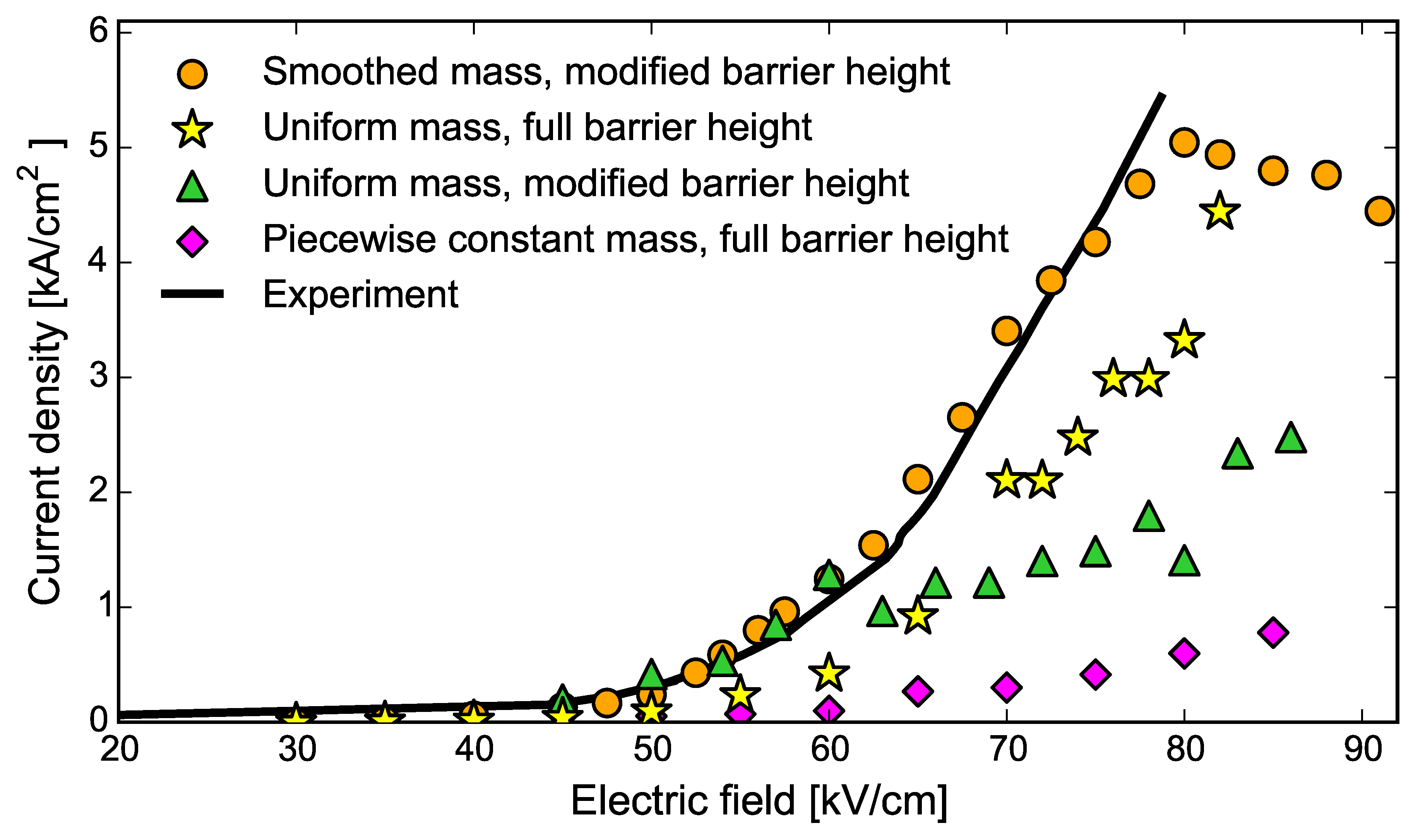
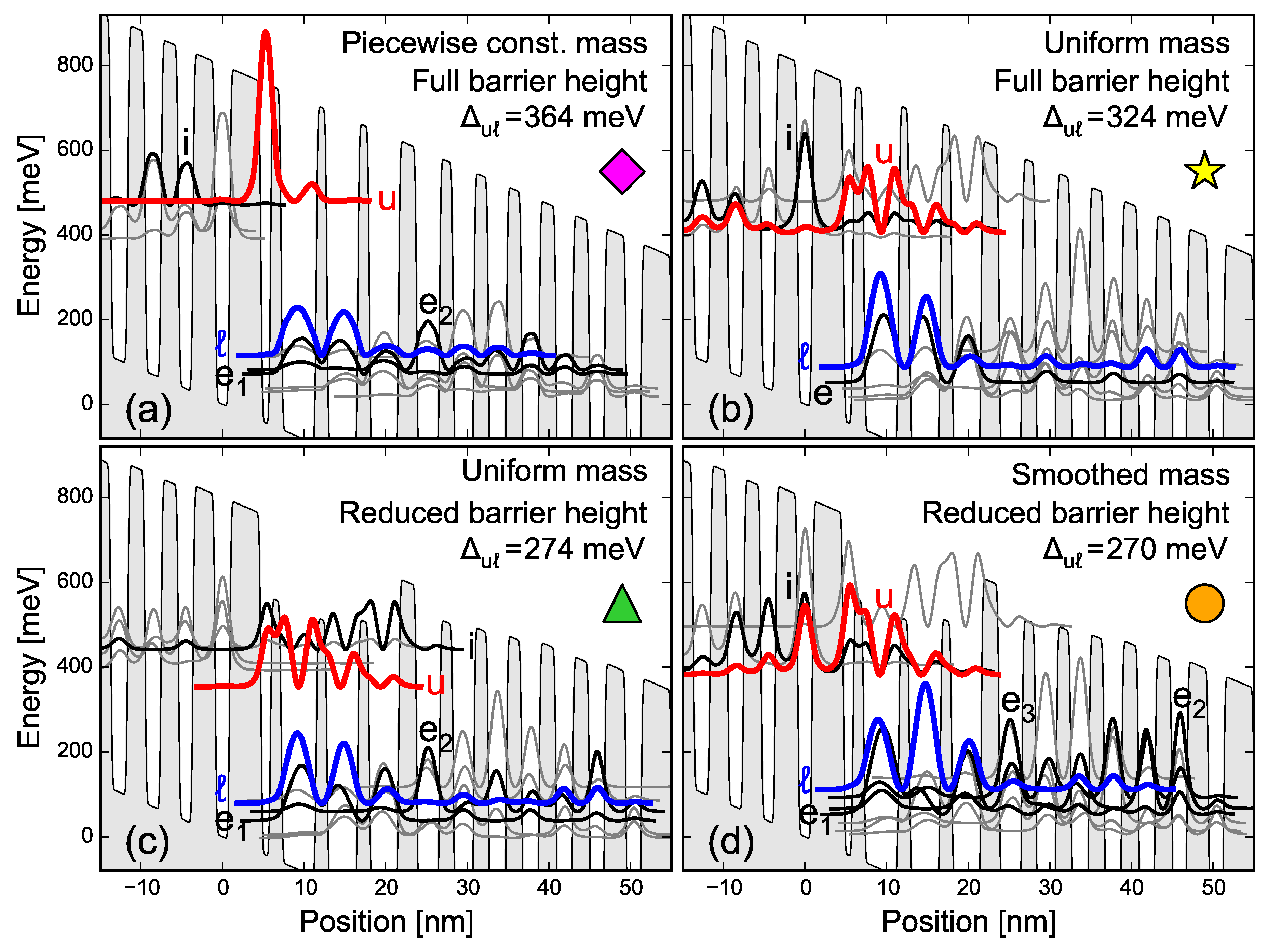
Figure 1 shows the sensitivity of the band structure to the effective mass and to the barrier height in the active region, where several thin barriers are found. The corresponding current density versus field ($J–F$) curves are presented in Figure 2 and illustrate how the effective mass and barrier height choice would manifest in these experimentally accessible characteristics. We now analyze this data in detail.

Figure 1a shows the calculated band structure at the design electric field (82 kV/cm) using a piecewise-constant effective mass (the effective mass changes abruptly at well/barrier interfaces). The well and barrier materials have effective masses of $0.0356$ and $0.104$ of the electron rest mass, respectively (barrier effective mass is obtained by linear interpolation between AlAs and InAs). The conduction band discontinuity between the two materials has been estimated to be approximately 800 meV [39]. The most striking feature in Figure 1a is that we obtain an energy difference ${\mathsf{\Delta }}_{u\ell }=364$ meV between the upper (u) and lower (ℓ) lasing level, which is $35\%$ higher than the experimentally observed value of 270 meV. There is very little overlap between the injector states and the upper lasing level, resulting in inefficient injection. These shortcomings are reflected in the $J–F$ curve in Figure 2 (purple diamonds), where the room-temperature current density is about 10 times lower than in experiment and we do not observe population inversion in transport simulations. It is clear that modeling the effective mass as piecewise-constant does not give satisfactory results. However, this approach has been used successfully to describe GaAs/AlGaAs-based devices [32] as well as devices based on lattice-matched InGaAs/InAlAs [34]. A possible explanation is that in the cases of GaAs/Al${}_x$Ga${}_{1-x}$As and lattice-matched InGaAs/InAlAs, the difference in effective masses is smaller. For example, the ratio of the effective masses in Al${}_{0.25}$Ga${}_{0.75}$As and GaAs is about $1.3$, while the ratio is about $1.4$ for lattice-matched InGaAs/InAlAs. On the other hand, the ratio of the effective masses of In${}_{0.362}$Al${}_{0.638}$As and In${}_{0.669}$Ga${}_{0.331}$As is about $2.9$. Another aspect is that the considered structure is highly strained, which affects effective mass.

Figure 1b shows the band structure calculated assuming a uniform effective mass, given by the weighted average of the well and barrier effective masses; the weight of well (barrier) mass is the total thickness of wells (barriers) in a stage divided by the stage length. We can see that the band structure is much more favorable to lasing, with an injector state that efficiently injects into the upper lasing level. The corresponding $J–F$ curve in Figure 2 (yellow stars) has a fairly good agreement with experiments, and we observe a population inversion in transport simulations. However, the calculated energy seperation between the upper and lower lasing levels at the design field of 82 kV/cm is 324 meV, about $20\%$ higher than in experiments.

The energy of the upper lasing level is very sensitive to the height of the potential barriers in the active region (the three barriers to the right of the injector barrier) because the upper lasing level has a high amplitude in the classically forbidden region inside the barriers. These barriers are only several monolayers thick ($1.3$–$1.4$ nm), and it is plausible that they do not reach the bulk value of the conduction band discontinuity (800 meV). Figure 1c shows the calculated band structure assuming a uniform effective mass and a barrier height V that depends on the barrier thickness W as

$$\begin{array}{c}\hfill V=V_0\left(1-e^{-W^2/W_0^2}\right)\end{array}$$

(3)

where $V_0=800$ meV is the full barrier height and $W_0=1.08$ nm, which is between three and four monolayers. This specific value of $W_0$ was chosen because it gives an energy difference ${\mathsf{\Delta }}_{u\ell }=274$ meV at the design electric field, which is within $2\%$ of the experimentally observed value of 270 meV. However, using this approach, the injector state cannot inject efficiently into the upper lasing level, the calculated current density shown in Figure 2 (green triangles) is three times lower than in experiment, and we do not observe a population inversion between the upper and lower lasing levels in transport simulations.

Figure 1d shows the calculated band structure with the thickness-dependent barrier height (Equation (3), as in Figure 1c), but with a middle ground between uniform and piecewise-constant mass: we assume a position-dependent effective mass, given by

$$\begin{array}{c}\hfill m^{*}\left(z\right)=\frac{1}{\sqrt{\pi }\sigma }\int e^{-{(z-z^{\prime })}^2/{\sigma }^2}{m}_{pc}^{*}\left(z^{\prime }\right)d{z}^{\prime }\end{array}$$

(4)

where $m_{pc}^{*}\left(z\right)$ is a piecewise-constant effective mass and σ is a smoothing length. The smoothing length affects the relative energy difference between the injector state and the upper lasing level. A smoothing length of σ = 8 nm results in the best alignment between these two states at the predicted design electric field [8]. Smoothing qualitatively captures the effects of strain and barrier thinness on the effective mass. With a smoothed mass, an electron is heavier in the injector, where the InAlAs barriers (with higher bulk mass) dominate, and lighter in the active region, with more InGaAs wells (regions with lower bulk mass). By smoothing the mass, the states localized in the injector (where electrons are now heavier, and energies roughly follow $\sim 1/m^{*}$) are lowered and brought into alignment with the upper lasing level, without the energy difference ${\mathsf{\Delta }}_{u\ell }$ being considerably affected. From the band structure in Figure 1d, we can see that the lasing energy is within 1 meV of the experimentally observed value and the overlap between the upper lasing level and the injection level is favorable for efficient injection. The simulated room-temperature $J–F$ curve in Figure 2 (orange circles) shows excellent agreement with experiment.

The approximations of a smoothed, position-dependent effective mass and barrier-height reduction in very thin layers are intuitively plausible: they capture the fact that properties that characterize bulk materials, such as the effective masses and band offsets, cannot be guaranteed to hold within layers that are only 3–4 monolayers thick. Further experimental studies are needed to benchmark the degree of energy barrier lowering in thin layers.

We note that an energy-dependent effective mass has been been employed previously to calculate the band structure and transport in QCLs [33,36,40,41], but this is not a viable option within our approach. An energy-dependent effective mass makes the Schrödinger Equation (2) effectively a nonlinear eigenvalue problem [40,41], so the eigenstates associated with different energies are no longer guaranteed to be orthogonal. However, orthogonality of the eigenstates is an absolutely critical property in the derivation of the master equation for the density matrix, specifically in the derivation of the dissipative term [32,38,42]. With a nonorthonormal eigenbasis of the Hamiltonian without scattering, the positivity of the density matrix upon evolution according to a master equation would no longer be guaranteed, which can lead to unphysical behavior. This further justifies the approximation of a smoothed, position-dependent effective mass within the presented approach.

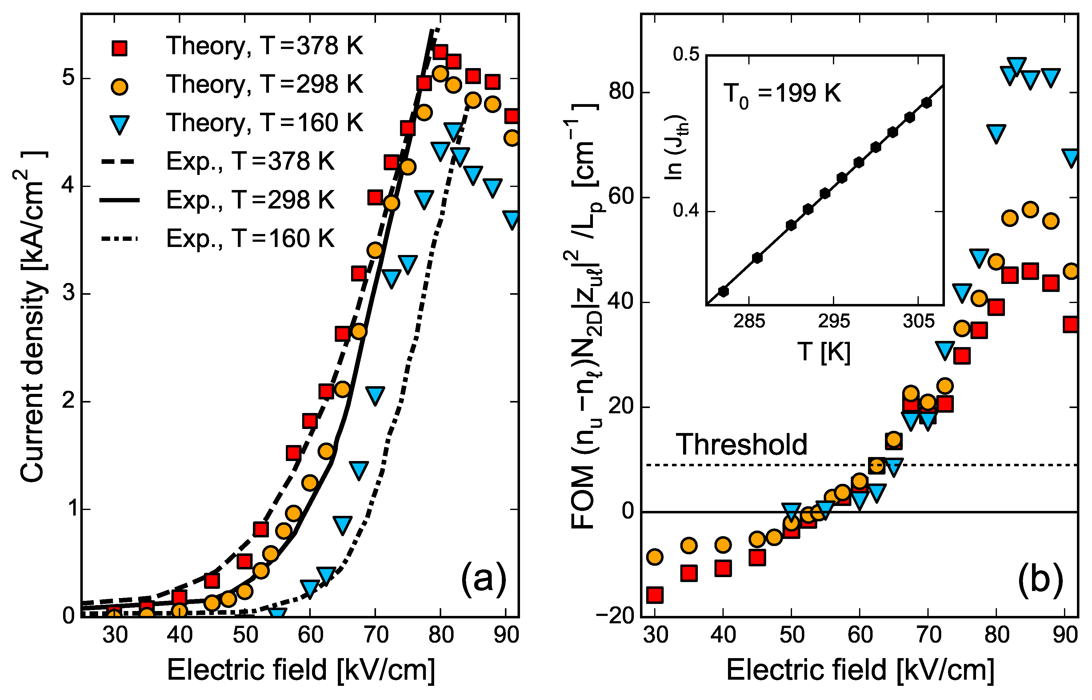
Figure 3a shows a comparison between the calculated current density and experiment at different temperatures. All calculations henceforth have a smoothed effective mass and modified barriers heights, as in Figure 1, and assume a temperature equal to the experimental heat-sink temperature (in reality, some lattice heating takes place). We obtain very good agreement with measured current density at 298 K and 378 K; however, the calculation somewhat overestimates the current density at 160 K. The difference between theory and experiment at low temperatures can be explained by the increased relative importance of interface roughness, alloy, and impurity scattering (not included in our model) at low temperatures.

Figure 3b shows the figure of merit (FOM), given by Equation (1d), versus field at different temperatures. For temperatures of 298 k and 378 K, the largest FOM is reached for the field strength of 85 kV/cm, which is in the negative differential resistance (NDR) region and beyond the maximum experimental field strength. However, at a temperature of 160 K, the onset of NDR is shifted to higher fields (83 kV/cm) and experimental results are provided up to $84.5$ kV/cm, reaching the field strength of maximum predicted gain. This result could be a factor in the much greater device performance at 160 K, where emitted power of $3.25$ W was measured, compared with $1.3$ W at room temperature [8].

The considered device was reported to have a threshold current density $J_{\mathrm{th}}=1.53$ kA/cm${}^2$ at room temperature (298 K) [8]. A comparison between Figure 3a,b shows that this value of current density corresponds to a field of $62.5$ kV/cm and a $\text{FOM}=9$ cm${}^{-1}$, which is close to the onset of population inversion (54 kV/cm). Note that the FOM is not modal gain; it is proportional to modal gain, with a proportionality constant that is weakly temperature dependent. We therefore define ${\text{FOM}}_{\mathrm{th}}=9$ cm${}^{-1}$ as a criterion for the onset of lasing. Then, we calculate the threshold current density $J_{\mathrm{th}}\left(T\right)$ as the current corresponding to the field that yields ${\text{FOM}}_{\mathrm{th}}$, which enables us to compute $J_{\mathrm{th}}\left(T\right)$ for temperatures around 298 K. The calculated temperature variation follows $J_{\mathrm{th}}\left(T\right)=J_0{e}^{T/T_0}$, as depicted in the inset to Figure 3b, which shows $ln\left(J_{\mathrm{th}}\right)$ vs. T near room temperature. The slope of the best linear fit yields $T_0=199$ K; the experiment gives 143 K. The discrepancy between between experiment and theory can be attributed to the omission of alloy, interface, and impurity scattering, and to lack of nonequilibrium phonons [25]. We note that a prior study [43] of the structure in [8], which employed rate equations, the effect of elastic scattering on lifetimes and electroluminescence linewidth, and upper-level electronic temperatures based on Vitiello et al.’s [44] measurement of the electron-lattice coupling constant on 4.8-$\mathsf{\mu }$m-emitting conventional QCL, gave a $T_0$ value of 167 K.

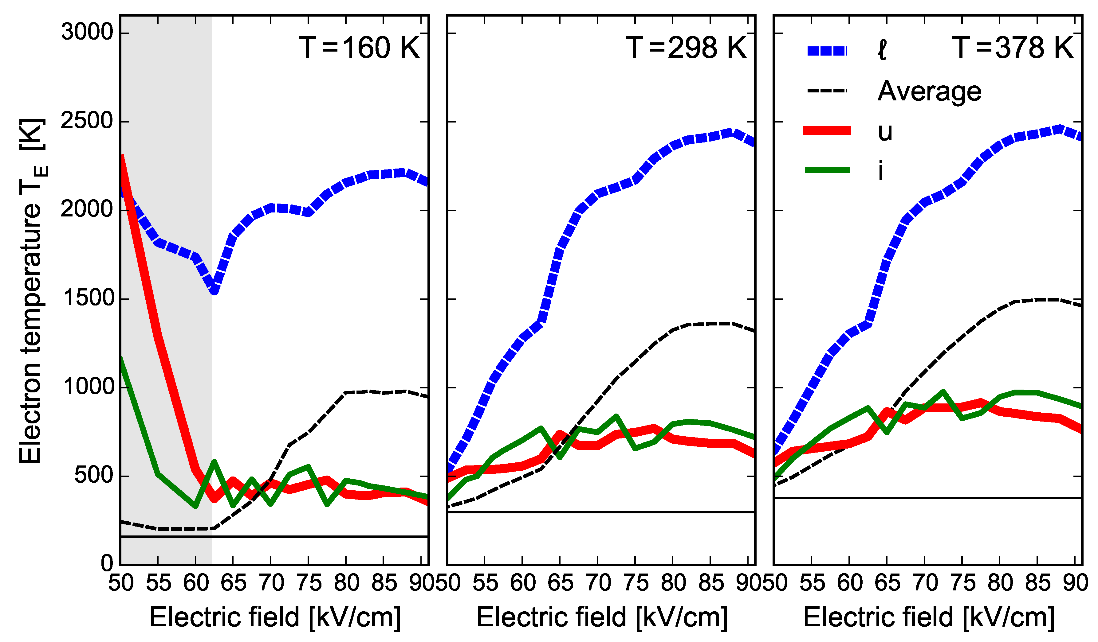
Figure 4 shows the subband electron temperatures (measuring the average in-plane kinetic energy of electrons in a subband, Equation (1e)) in the injector, upper lasing, and lower lasing levels, as a function of electric field for lattice temperatures of 160 K (left), 298 K (middle), and 378 K (right). Also shown is the weighted average electron temperature for a stage, with subband occupations acting as weights. Significant electron heating takes place: the weighted average electron temperature around the design field ($\sim 80$ kV/cm) is between 1000 and 1500 K. The injector and upper lasing levels are cooler than average, with electron temperatures between 400 K and 1000 K around the design field. These high electron temperatures in the upper lasing state will increase carrier leakage and impact the $T_0$ value [43]. The lower lasing level is considerably hotter than average, with electron temperatures in the range 2200 to 2400 K; the extractor states (not shown) have comparable temperatures to the lower lasing level. The high electron temperature in the lower lasing level is intuitively plausible: this level is populated by electrons that scattered from the upper to the lower lasing level and thus possess approximately 240 meV of excess kinetic energy (240 meV corresponds to a temperature of $\sim 2800$ K) [45].

The low-field trends at 160 K differ from higher lattice temperatures because the upper and injector states have practically no occupation, so their electronic temperature calculated as the subband ensemble average of kinetic energy is not meaningful; this is implied by the boxed gray region in the left panel. The (meaningless) high temperature comes from the very few electrons that scatter into the two states and scatter out quickly, before they have enough time to thermalize. At low lattice temperature and field, practically all the electrons ( 95%) are in the lowest energy state in the injector (not shown in Figure 4). This state is “cold” and, because of its high occupation, it determines the average electron temperature for all subbands, which is why the average electron temperature is lower than those of u, ℓ, and i. However, at higher lattice temperatures, electrons can access u and i from from the injector ground state via polar optical phonon absorption; the population of these subbands becomes appreciable and the electron temperature becomes a more meaningful measure of the average electron energy in these subbands.

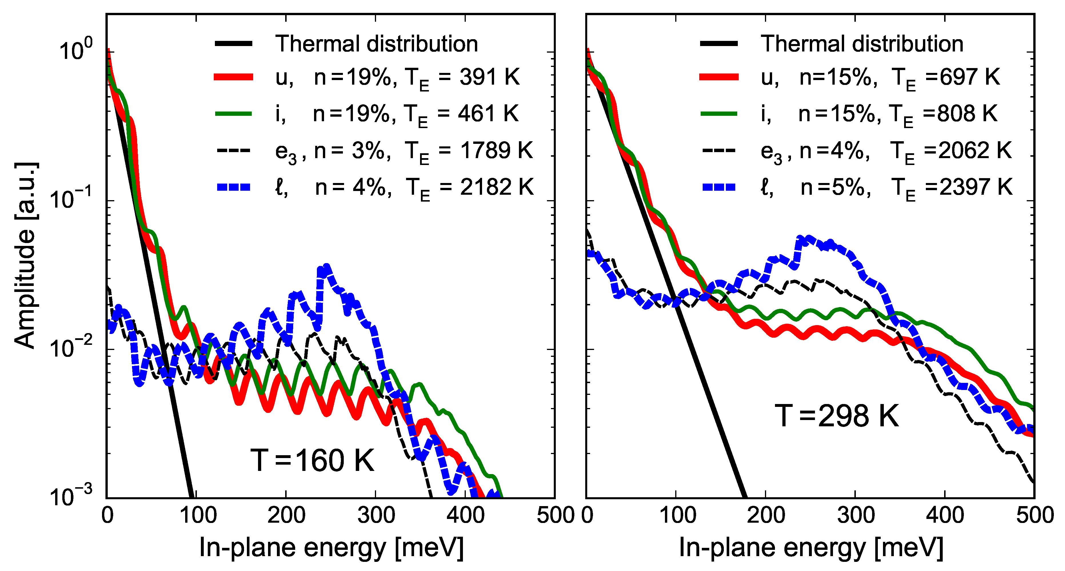
Figure 5 shows the in-plane energy distribution for different subbands at a field strength of 82 kV/cm, for lattice temperatures of 160 K (left panel) and 298 K (right panel). Nonthermal electron distributions have been obtained previously using both semiclassical and quantum transport approaches for various QCL structures in the mid-IR [25,33,46,47]. The in-plane distributions for the injector and upper lasing levels have similar shapes: at low energies (0–100 meV), both distributions are well described by a heated Maxwellian (i.e., they are linear in these semilog plots). However, at higher energies, both distributions have a broad tail, which is reflected in the high electron temperatures of the injector and upper lasing levels (391 to 461 K, respectively, and for the lattice temperature of 160 K, and 697 to 808 K, respectively, at the lattice temperature of 298 K). Neither the lower lasing level nor the $e_3$ extractor distributions resemble a Maxwellian. Both states have nearly flat distributions, reaching up to the photon energy of 270 meV and yielding very high electron temperatures (up to 2397 K for the lower lasing level for a lattice temperature of 298 K). All in-plane distributions exhibit oscillations with a period equal to the optical phonon energy of 32 meV (also observed in NEGF simulations [36]). The oscillations are more prominent at low temperatures; electron–electron scattering, which we did not account for but which is generally important at low temperatures, would help randomize in-plane energy and smoothen out these oscillations.

While distributions over in-plane energy are clearly nonthermal, we note that the effective electronic temperature, being a single parameter, enables us to compare characteristic subband energies between different subbands across different electric fields and heat-sink temperatures. Subband electronic temperatures are very useful in building intuition about quantities related to characteristic electronic kinetic energy (e.g., the backfilling current, the shunt-type leakage currents within the active region, the rate of escape into the continuum), which are widely used in simplified phenomenological models and greatly help with QCL design.

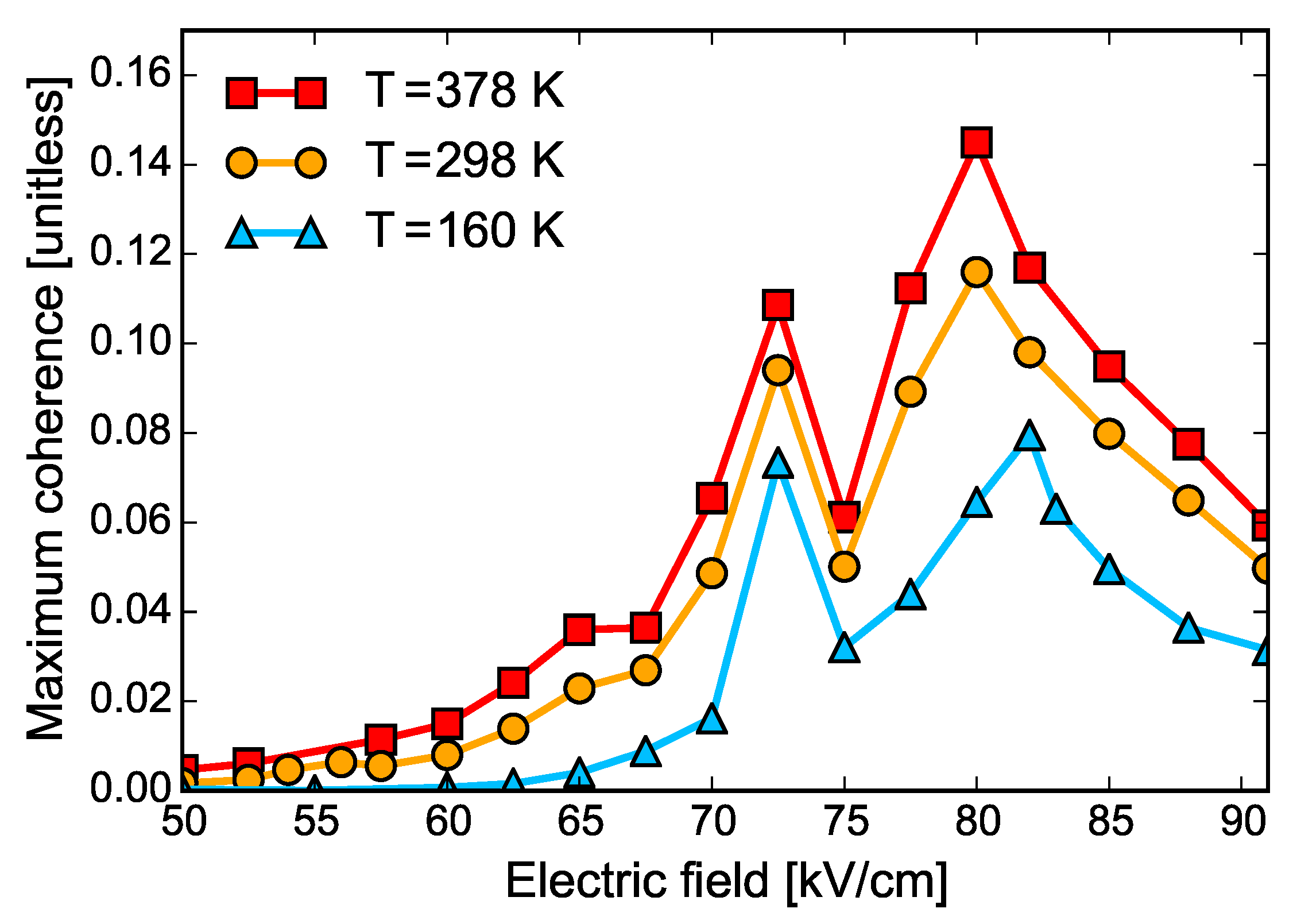
Figure 6 shows the magnitude of the ratio of the largest coherence ${\rho }_{ij}$ with $i\ne j$ to the largest diagonal density-matrix element ${\rho }_{ii}$. This quantity gives us an idea of the importance of including coherences in the model. We see that coherences can be up to $15\%$ of the largest diagonal matrix element and that coherences are highest around the design lasing field of 82 kV/cm. The peak around 80–82 kV/cm is due to the coherence between the upper lasing level and the injector state. The coherence peak around 72 kV/cm is due to two states localized in the injector region. Large coherences arise when two states have considerable spatial overlap and a small energy difference, which is clearly the case for the upper lasing state and the injector state at 82 kV/cm (see Figure 1d). We note that this alignment is known to be very problematic in semiclassical simulations, leading to numerical spikes in current. This level crossing is recognized as very important in density-matrix simulations, but usually treated phenomenologically [27,30,34,37]. Here, our approach is based on a rigorous density-matrix framework, where treatment of coherences is accurate and on an equal footing with the occupations. We conclude that, in order to accurately model injection in QCLs, it is critical to include the coherence between the injector state into the upper lasing level.

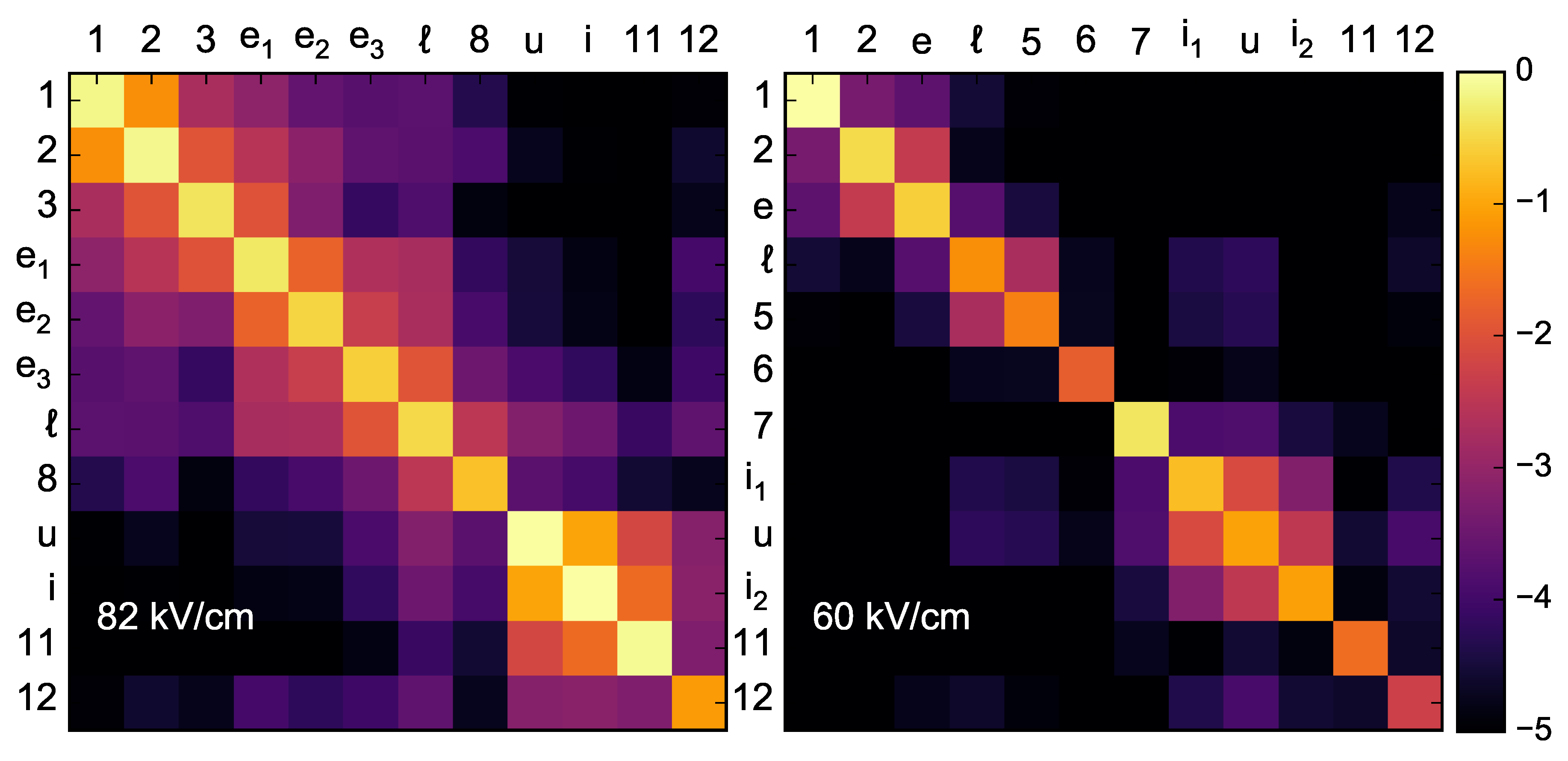
Figure 7 shows a plot of log${}_{10}\left(\right|{\rho }_{ij}\left|\right)$ around lasing for a lattice temperature of 298 K and a field strength of 82 kV/cm (left panel). Important states are given labels, while other states’ thin gray curves in Figure 1d are given numbers in order of increasing energy. Normalization is chosen such that the greatest diagonal value is one. Around the design lasing field, the greatest coherence is between the injector and upper lasing level (${\rho }_{iu}$) and is about $10\%$ of the largest diagonal element. The second largest coherence is ${\rho }_{12}$ ($6\%$) and all other coherences are smaller than $2.5\%$ of the largest diagonal element. The greatest coherence involving the lower lasing level is ${\rho }_{\ell e_3}$, which means the lower lasing level couples most strongly to the $e_3$ extractor state, which, in turn, means that $e_3$ is the most effective extractor state. The right panel of Figure 7 shows the density matrix for a field strength of 60 kV/cm, which is slightly below threshold ($62.5$ kV/cm). It is apparent that the coherences are considerably smaller at lower fields. The corresponding band structure is not shown, but the most important states are labeled. The greatest coherences are again between the upper lasing level and the injector states (there are two efficient injector states, $i_1$ and $i_2$, at this field). The greatest coherences are $0.8\%$, between the upper lasing level and the $i_1$ injector state (${\rho }_{u{i}_1}$). The coherence between the lower lasing level and the extractor state has a magnitude of $0.01\%$, indicating very inefficient extraction from the lower lasing level. It is noteworthy that coherences are very small overall at this near-threshold field, which indicates that a semiclassical transport description would be fairly accurate. In contrast, a semiclassical simulation is unlikely to be accurate for the description of transport at the design lasing field. This finding amends the conventional wisdom that transport in mid-IR QCL is largely incoherent and sheds light on the great importance of coherences, particularly in describing the injection process.

4. Conclusions

We presented a quantum transport simulation of a 4.6-$\mathsf{\mu }$m QCL operating at high power near room temperature. The simulation is based on a rigorous density-matrix-based formalism, in which the evolution of the single-electron density matrix follows a Markovian master equation in the presence of the applied field and relevant scattering mechanisms.

We showed that, in these structures—which have strained layers, very thin barriers, and a great electron-mass disparity between the wells and the barriers—that it may be important to allow for both position-dependent effective mass and for effective lowering of very thin barriers in order to obtain the band structure and the $J–F$ characteristics comparable to experiments. Our calculations have predictive value and agree well with experiments over a wide range of temperatures. We predicted a room-temperature threshold field of $62.5$ kV/cm and a characteristic temperature for threshold-current-density variation of $T_0=199\mathrm{K}$, somewhat higher than experiments but very reasonable for a QCL in this wavelength range.

Furthermore, we showed that the electronic in-plane distributions are far from thermal, featuring wide non-Maxwellian tails. This finding indicates that assuming thermal distributions, which is commonly done in semiphenomenological density-matrix approaches, is not well justified. We computed effective electron temperatures from the average in-plane energy for a given subband over a range of fields; at the design electric field, the temperatures can be hundreds to thousands of degrees higher than the heat sink.

Finally, we emphasized the role of coherent, tunneling current by looking at the size of coherences, the off-diagional elements of the density matrix. At the design lasing field, efficient injection manifests itself in a large injector/upper lasing level coherence, which underscores the insufficiency of semiclassical techniques to address injection in QCLs.

The novelty of our work is in demonstrating a density-matrix approach where the decoherence and dephasing are rigorously captured, with a completely positive Markovian map, by applying it to this experimentally well-characterized QCL system. Quantum transport simulation based on the density-matrix approach, especially if implemented with a rigorous dissipative term [32,38,48] instead of phenomenologically [27,30,34,37], is a numerically efficient alternative to NEGF in addressing partially coherent transport in high-power, short-wavelength QCLs.

References

1. Faist, J.; Capasso, F.; Sivco1, D.L.; Sirtori, C.; Hutchinson, A.L.; Cho, A.Y. Quantum Cascade Laser. Science 1994, 264, 553–556. [Google Scholar] [CrossRef] [PubMed]
2. Faist, J. Wallplug efficiency of quantum cascade lasers: Critical parameters and fundamental limits. Appl. Phys. Lett. 2007, 90, 253512. [Google Scholar] [CrossRef]
3. Yao, Y.; Hoffman, A.J.; Gmachl, C.F. Mid-infrared quantum cascade lasers. Nat. Photonics 2012, 6, 432. [Google Scholar] [CrossRef]
4. Botez, D.; Chang, C.; Mawst, L. Temperature Sensitivity of the Electro-Optical Characteristics for Mid-Infrared (λ = 3-16 μm)-Emitting Quantum Cascade Lasers. J. Phys. D Appl. Phys. 2016, 49, 043001. [Google Scholar] [CrossRef]
5. Capasso, F. High-performance midinfrared quantum cascade lasers. Opt. Eng. 2010, 49, 111102. [Google Scholar] [CrossRef]
6. Razeghi, M.; Bandyopadhyay, N.; Bai, Y.; Lu, Q.; Sliveken, S. Recent advances in mid infrared (3–5 μm) quantum cascade lasers. Opt. Materials Express 2013, 3, 1872. [Google Scholar] [CrossRef]
7. Bai, Y.; Bandyopadhyay, N.; Tsao, S.; Slivken, S.; Razeghi, M. Room temperature quantum cascade lasers with 27% wall plug efficiency. Appl. Phys. Lett. 2011, 98, 181102. [Google Scholar] [CrossRef]
8. Bai, Y.; Darvish, S.R.; Slivken, S.; Zhang, W.; Evans, A.; Nguyen, J.; Razeghi, M. Room temperature continuous wave operation of quantum cascade lasers with watt-level optical power. Appl. Phys. Lett. 2008, 92, 101105. [Google Scholar] [CrossRef]
9. Lyakh, A.; Maulini, R.; Tsekoun, A.; Go, R.; Pflügl, C.; Diehl, L.; Wang, Q.J.; Capasso, F.; Patel, C.K.N. 3 W continuous-wave room temperature single-facet emission from quantum cascade lasers based on nonresonant extraction design approach. Appl. Phys. Lett. 2009, 95, 141113. [Google Scholar] [CrossRef]
10. Bandyopadhyay, N.; Bai, Y.; Gokden, B.; Myzaferi, A.; Tsao, S.; Slivken, S.; Razeghi, M. Watt level performance of quantum cascade lasers in room temperature continuous wave operation at λ∼3.76 μm. Appl. Phys. Lett. 2010, 97, 131117. [Google Scholar] [CrossRef]
11. Bandyopadhyay, N.; Slivken, S.; Bai, Y.; Razeghi, M. High power continuous wave, room temperature operation of λ∼3.4 μm and λ∼3.55 μm InP-based quantum cascade lasers. Appl. Phys. Lett. 2012, 100, 212104. [Google Scholar] [CrossRef]
12. Bandyopadhyay, N.; Bai, Y.; Tsao, S.; Nida, S.; Slivken, S.; Razeghi, M. Room temperature continuous wave operation of λ∼3–3.2 μm quantum cascade lasers. Appl. Phys. Lett. 2012, 101, 241110. [Google Scholar] [CrossRef]
13. Zhang, Q.; Liu, F.Q.; Zhang, W.; Lu, Q.; Wang, L.; Li, L.; Wang, Z. Thermal induced facet destructive feature of quantum cascade lasers. Appl. Phys. Lett. 2010, 96, 141117. [Google Scholar] [CrossRef]
14. Botez, D.; Shin, J.C.; Kirch, J.D.; Chang, C.C.; Mawst, L.J.; Earles, T. Multidimensional Conduction-Band Engineering for Maximizing the Continuous-Wave (CW) Wallplug Efficiencies of Mid-Infrared Quantum Cascade Lasers. IEEE J. Sel. Topics Quantum Electron. 2013, 19, 1200312. [Google Scholar] [CrossRef]
15. Lee, H.K.; Yu, J.S. Thermal analysis of short wavelength InGaAs/InAlAs quantum cascade lasers. Solid-State Electron. 2010, 54, 769. [Google Scholar] [CrossRef]
16. Wienold, M.; Semtsiv, M.P.; Bayrakli, I.; Masselink, W.T.; Ziegler, M.; Kennedy, K.; Hogg, R. Optical and thermal characteristics of narrow-ridge quantum-cascade lasers. J. Appl. Phys. 2008, 103, 083113. [Google Scholar] [CrossRef]
17. Kirch, J.D.; Shin, J.C.; Chang, C.C.; Mawst, L.J.; Botez, D.; Earles, T. Tapered active-region quantum cascade lasers (λ = 4.8 μm) for virtual suppression of carrier-leakage currents. Electron. Lett. 2012, 48, 234. [Google Scholar] [CrossRef]
18. Jirauschek, C.; Kubis, T. Modeling techniques for quantum cascade lasers. Appl. Phys. Rev. 2014, 1, 011307. [Google Scholar] [CrossRef]
19. Indjin, D.; Harrison, P.; Kelsall, R.; Ikonić, Z. Self-consistent scattering theory of transport and output characteristics of quantum cascade lasers. J. Appl. Phys. 2002, 91, 9019–9026. [Google Scholar] [CrossRef]
20. Indjin, D.; Harrison, P.; Kelsall, R.; Ikonić, Z. Influence of leakage current on temperature performance of GaAs/AlGaAs quantum cascade lasers. Appl. Phys. Lett. 2002, 81, 400–402. [Google Scholar] [CrossRef]
21. Mircetic, A.; Indjin, D.; Ikonic, Z.; Harrison, P.; Milanovic, V.; Kelsall, R.W. Towards automated design of quantum cascade lasers. J. Appl. Phys. 2005, 97, 084506. [Google Scholar] [CrossRef]
22. Iotti, R.; Rossi, F. Nature of Charge Transport in Quantum-Cascade Lasers. Phys. Rev. Lett. 2001, 87, 146603. [Google Scholar] [CrossRef] [PubMed]
23. Callebaut, H.; Kumar, S.; Williams, B.S.; Hu, Q.; Reno, J.L. Importance of electron-impurity scattering for electron transport in terahertz quantum-cascade lasers. Appl. Phys. Lett. 2004, 84, 645–647. [Google Scholar] [CrossRef]
24. Gao, X.; Botez, D.; Knezevic, I. X-valley leakage in GaAs-based midinfrared quantum cascade lasers: A Monte Carlo study. J. Appl. Phys. 2007, 101, 063101. [Google Scholar] [CrossRef]
25. Shi, Y.B.; Knezevic, I. Nonequilibrium phonon effects in midinfrared quantum cascade lasers. J. Appl. Phys. 2014, 116, 123105. [Google Scholar] [CrossRef]
26. Willenberg, H.; Döhler, G.H.; Faist, J. Intersubband gain in a Bloch oscillator and quantum cascade laser. Phys. Rev. B 2003, 67, 085315. [Google Scholar] [CrossRef]
27. Kumar, S.; Hu, Q. Coherence of resonant-tunneling transport in terahertz quantum-cascade lasers. Phys. Rev. B 2009, 80, 245316. [Google Scholar] [CrossRef]
28. Weber, C.; Wacker, A.; Knorr, A. Density-matrix theory of the optical dynamics and transport in quantum cascade structures: The role of coherence. Phys. Rev. B 2009, 79, 165322. [Google Scholar] [CrossRef]
29. Dupont, E.; Fathololoumi, S.; Liu, H. Simplified density-matrix model applied to three-well terahertz quantum cascade lasers. Phys. Rev. B 2010, 81, 205311. [Google Scholar] [CrossRef]
30. Terazzi, R.; Faist, J. A density matrix model of transport and radiation in quantum cascade lasers. New J. Phys. 2010, 12, 033045. [Google Scholar] [CrossRef]
31. Lee, S.C.; Wacker, A. Nonequilibrium Green’s function theory for transport and gain properties of quantum cascade structures. Phys. Rev. B 2002, 66, 245314. [Google Scholar] [CrossRef]
32. Jonasson, O.; Karimi, F.; Knezevic, I. Partially coherent electron transport in terahertz quantum cascade lasers based on a Markovian master equation for the density matrix. J. Comp. Electron 2016. to appear. [Google Scholar]
33. Mátyás, A.; Lugli, P.; Jirauschek, C. Photon-induced carrier transport in high efficiency midinfrared quantum cascade lasers. J. Appl. Phys. 2011, 110, 013108. [Google Scholar] [CrossRef]
34. Lindskog, M.; Wolf, J.M.; Trinite, V.; Liverini, V.; Faist, J.; Maisons, G.; Carras, M.; Aidam, R.; Ostendorf, R.; Wacker, A. Comparative analysis of quantum cascade laser modeling based on density matrices and non-equilibrium Green’s functions. Appl. Phys. Lett. 2014, 105, 103106. [Google Scholar] [CrossRef]
35. Bugajski, M.; Gutowski, P.; Karbownik, P.; Kolek, A.; Hałdaś, G.; Pierściński, K.; Pierścińska, D.; Kubacka-Traczyk, J.; Sankowska, I.; Trajnerowicz, A.; et al. Mid-IR quantum cascade lasers: Device technology and non-equilibrium Green’s function modeling of electro-optical characteristics. Phys. Status Solidi 2014, 251, 1144–1157. [Google Scholar] [CrossRef]
36. Kolek, A.; Haldas, G.; Bugajski, M.; Pierscinski, K.; Gutowski, P. Impact of Injector Doping on Threshold Current of Mid-Infrared Quantum Cascade Laser—Non-Equilibrium Green’s Function Analysis. IEEE J. Sel. Top. Quantum Electron. 2015, 21, 124–133. [Google Scholar] [CrossRef]
37. Callebaut, H.; Hu, Q. Importance of coherence for electron transport in terahertz quantum cascade lasers. J. Appl. Phys. 2005, 98, 104505. [Google Scholar] [CrossRef]
38. Heinz-Peter Breuer, F.P. The Theory of Open Quantum Systems; Oxford University Press: New York, NY, USA, 2002. [Google Scholar]
39. Evans, A.; Darvish, S.R.; Slivken, S.; Nguyen, J.; Bai, Y.; Razeghi, M. Buried heterostructure quantum cascade lasers with high continuous-wave wall plug efficiency. Appl. Phys. Lett. 2007, 91, 071101. [Google Scholar] [CrossRef]
40. Sirtori, C.; Capasso, F.; Faist, J.; Scandolo, S. Nonparabolicity and a sum rule associated with bound-to-bound and bound-to-continuum intersubband transitions in quantum wells. Phys. Rev. B 1994, 50, 8663. [Google Scholar] [CrossRef]
41. Cooper, J.; Valavanis, A.; Ikonić, Z.; Harrison, P.; Cunningham, J. Finite difference method for solving the Schrödinger equation with band nonparabolicity in mid-infrared quantum cascade lasers. J. Appl. Phys. 2010, 108, 113109. [Google Scholar] [CrossRef]
42. Karimi, F.; Davoody, A.H.; Knezevic, I. Dielectric function and plasmons in graphene: A self-consistent-field calculation within a Markovian master equation formalism. Phys. Rev. B 2016, 93, 205421. [Google Scholar] [CrossRef]
43. Botez, D.; Kumar, S.; Shin, J.C.; Mawst, L.J.; Vurgaftman, I.; Meyer, J.R. Temperature dependence of the key electro-optical characteristics for midinfrared emitting quantum cascade lasers. Appl. Phys. Lett. 2010, 97, 071101, Erratum: Appl. Phys. Lett. 2010, 97, 199901. [Google Scholar] [CrossRef]
44. Vitiello, M.S.; Gresch, T.; Lops, A.; Spagnolo, V.; Scamarcio, G.; Hoyler, N.; Giovannini, M.; Faist, J. Influence of InAs, AlAs δ layers on the optical, electronic, and thermal characteristics of strain-compensated GaInAs/AlInAs quantum-cascade lasers. Appl. Phys. Lett. 2007, 91, 161111. [Google Scholar] [CrossRef]
45. Harrison, P.; Indjin, D.; Kelsall, R.W. Electron temperature and mechanisms of hot carrier generation in quantum cascade lasers. J. Appl. Phys. 2002, 92, 6921–6923. [Google Scholar] [CrossRef]
46. Faist, J.; Hofstetter, D.; Beck, M.; Aellen, T.; Rochat, M.; Blaser, S. Bound-to-continuum and two-phonon resonance, quantum-cascade lasers for high duty cycle, high-temperature operation. IEEE J. Quantum Electron. 2002, 38, 533–546. [Google Scholar] [CrossRef]
47. Kolek, A.; Hałdaś, G.; Bugajski, M. Nonthermal carrier distributions in the subbands of 2-phonon resonance mid-infrared quantum cascade laser. Appl. Phys. Lett. 2012, 101, 061110. [Google Scholar] [CrossRef]
48. Knezevic, I.; Novakovic, B. Time-dependent transport in open systems based on quantum master equations. J. Comput. Electron. 2013, 12, 363–374. [Google Scholar] [CrossRef]
Figure 1. Calculated band structure using (a) piecewise constant mass with full barrier height, (b) uniform mass with full barrier height, (c) uniform mass with reduced barrier heights given by Equation (3), and (d) smoothed position-dependent effective mass given by Equation (4) with reduced barrier height given by Equation (3). For each case, the energy difference between upper and lower lasing levels Δ u is given. Labels identify the upper lasing level (u); lower lasing level (); most effective injector state (i), often referred to as the ground state; and notable extractor states ( e 1 , e 2 and e 3 , in increasing order of energy). The symbols (diamond, star, triangle, and circle) refer to the corresponding J F curves in Figure 2.
Photonics 03 00038 g001
Figure 2. Current density vs. electric field for the four band structures shown in Figure 1. All theoretical results are for a lattice temperature of 298 K, which we assume is the same as the heat-sink temperature in experiment [8].
Photonics 03 00038 g002
Figure 3. (a) Calculated (symbols) and measured (lines) current density vs. electric field characteristics at different temperatures (378, 298, and 160 K); (b) figure of merit (FOM) (proportional to modal gain) vs. electric field at different temperatures. The reported threshold current density of 1 . 53 kA/cm 2 at a temperature of 298 K corresponds to a field strength of 62 . 5 kV/cm and FOM th = 9 cm - 1 (dashed horizontal line), which is slightly above the onset of population inversion (54 kV/cm, FOM = 0). (Inset) Semilog plot of the threshold current density versus temperature (symbols) and a best linear fit ln ( J th ) = l n ( J 0 ) + T / T 0 with T 0 = 199 K (solid line). Experimental data from [8].
Photonics 03 00038 g003
Figure 4. Electron temperature in the upper, lower, and injector states as a function of electric field. Solid horizonal lines denote the lattice temperature. Note that the electron temperatures are not fitting parameters, but calculated using Equation (1e). Also shown is the weighted average (weights are occupations) of the electron temperatures of all subbands. In the grayed area for T = 160 K, the considered states had vanishing occupations, so the high electron temperatures at low fields are not meaningful.
Photonics 03 00038 g004
Figure 5. In-plane electron energy distribution for the upper lasing level (u), lower lasing level (), injector (i), and the most important extractor ( e 3 ) state. Results are shown at the design lasing field (82 kV/cm) for lattice temperatures of 160 K (left) and 298 K (right). The solid black line shows the corresponding thermal equilibrium distribution e - E k / k B T for comparison. For each state, the corresponding occupation n (percentage of stage occupation) and the calculated electron temperature T E are given in the legend.
Photonics 03 00038 g005
Figure 6. Ratio of the largest coherence to the largest occupation as a function of applied electric field. The peak around the design lasing field (80 kV/cm) is due to the coherence between the injector and upper lasing level. The peak around 72 kV/cm is due to two states localized in the injector region.
Photonics 03 00038 g006
Figure 7. A color map showing log 10 ( | ρ i j | ) for a lattice temperature of 298 K. Normalization is chosen such that the largest matrix element is 1. The left panel shows results around lasing (82 kV/cm) for all the states shown in the band structure in Figure 1d. Important states are labeled, while other states are given numbers in increasing order of energy. The right panel shows the same quantity, but for a field below lasing (60 kV/cm). The corresponding band structure is not shown; however, important states are given labels.
Photonics 03 00038 g007